Article

Drowsiness Estimation Using Electroencephalogram and Recurrent Support Vector Regression

by
Izzat Aulia Akbar
1 and
Tomohiko Igasaki
1,2,*
1
Department of Human and Environmental Informatics, Graduate School of Science and Technology, Kumamoto University, Kumamoto 860-8555, Japan
2
Field of Biomedical and Welfare Engineering, Division of Informatics and Energy, Faculty of Advanced Science and Technology, Kumamoto University, Kumamoto 860-8555, Japan
*
Author to whom correspondence should be addressed.
Information 2019, 10(6), 217; https://doi.org/10.3390/info10060217
Submission received: 24 May 2019 / Revised: 18 June 2019 / Accepted: 23 June 2019 / Published: 24 June 2019
(This article belongs to the Section Information Processes)

Abstract

:
As a cause of accidents, drowsiness can cause economical and physical damage. A range of drowsiness estimation methods have been proposed in previous studies to aid accident prevention and address this problem. However, none of these methods are able to improve their estimation ability as the length of time or number of trials increases. Thus, in this study, we aim to find an effective drowsiness estimation method that is also able to improve its prediction ability as the subject’s activity increases. We used electroencephalogram (EEG) data to estimate drowsiness, and the Karolinska sleepiness scale (KSS) for drowsiness evaluation. Five parameters (α, β/α, (θ+α)/β, activity, and mobility) from the O1 electrode site were selected. By combining these parameters and KSS, we demonstrate that a typical support vector regression (SVR) algorithm can estimate drowsiness with a correlation coefficient (R2) of up to 0.64 and a root mean square error (RMSE) of up to 0.56. We propose a “recurrent SVR” (RSVR) method with improved estimation performance, as highlighted by an R2 value of up to 0.83, and an RMSE of up to 0.15. These results suggest that in addition to being able to estimate drowsiness based on EEG data, RSVR is able to improve its drowsiness estimation performance.

1. Introduction

Drowsiness, the difficulty in maintaining consciousness, is a natural phenomenon experienced by human beings. In normal circumstances, it is caused by circadian rhythms, and is usually felt at night, as the state before sleep. However, when experienced during tasks at work that require concentration, or driving, drowsiness can cause harmful accidents. Therefore, drowsiness estimation needs investigation for such accidents to be prevented. Recently, a range of methods for detecting drowsiness have been proposed. By noting the tendency of people to yawn frequently when they felt sleepy, a study proposed a yawn detection-based estimation technique, in which a camera, for identifying when a driver yawns, is placed under a car’s interior mirror [1]. Drowsiness while driving can also be detected using a trajectory sensor [2,3] that monitors a vehicle’s movement, as a driver’s control becomes erratic if they are drowsy. Other researchers have proposed the use of biological data, such as electrocardiogram (ECG) [4,5,6], electrooculogram (EOG) [7,8,9], respiratory [10,11], electromyogram (EMG) [12] and electroencephalogram (EEG) [13,14,15,16] signals to assess drowsiness. In this study, we have selected EEG data as a parameter for assessing drowsiness, since it is fundamentally related to the activity of the human brain [17].
Prior studies have shown that EEG data can be used to detect drowsiness, which can be classified further on either a two or three-level scale [13,14,16]. However, these studies used a relatively big dataset to detect drowsiness and they did not consider improving their estimation performance as more of the subject’s activity was encountered. We hypothesize that in real conditions, training data are initially limited, although though these data will accumulate gradually as activity increases, and more scenarios are identified. However, the limited dataset available undermines the accuracy of estimation. Thus, a study investigating drowsiness estimation techniques, which use a limited dataset and can improve the estimation performance as more of a subject’s activity is encountered, is required. In previous studies where the initial baseline consisted of a limited dataset, estimation was completed using regression rather than classification methods, due to the ability of these techniques to approximate an output label outside the pre-defined range [18]. Likewise, we will employ support vector regression (SVR) as the basis for drowsiness estimation.
In this study, we employ a questionnaire to characterize drowsiness in nine levels, represented by the Karolinska sleepiness scale (KSS), ranging from very alert to very sleepy. Then, we propose a “recurrent SVR” (RSVR) technique to estimate the appropriate KSS level from EEG parameters obtained during simulated driving. Finally, we analyze if the RSVR technique is able to maintain or improve its estimation performance as more driving trials are gradually encountered, regardless of its initial reliance on a limited dataset.

2. Materials and Methods

2.1. Participants

Sixteen healthy males were selected to participate in this study (mean age: 23.06 ± 3.88 years old). All subjects were confirmed to have a valid driving license and gave their informed consent before the experiments. Subjects were also asked to have breakfast and lunch before each trial; sleep for at least 7.5 h the night before [19]; and to refrain from consuming any prescription medication, alcohol, caffeinated beverages, and from smoking [20,21] before the day of the experiment.

2.2. Tasks

Each participant completed all the experiments in four days. Two trials were assigned to the subjects in a day, with one conducted between 08:00 and 10:00 and the other between 13:00 and 15:00, such that eight trials were completed for each subject in total. In each trial, each subject was instructed to drive in a simulator (DA-110, Honda Motor, Tokyo, Japan) and maintain a speed of 100 km/h for 50 min. To induce drowsiness, we selected an oval track with no traffic obstacles. In addition, each subject was also instructed to remain in a resting state in the driving simulator’s seat, and asked to report their drowsiness condition every 30 s for a period of 5 min before and after each trial, in a direct observation process. During this period, the subjects’ facial expressions were recorded. Drowsiness evaluation was again conducted at a different time after the trial had finished, by asking the subject to complete a drowsiness questionnaire every 30 s for 5 min using this recorded footage, in an indirect observation process. These data were used as a validator for the similarity test in the statistical analysis. The questionnaire evaluation was carried out not only 5 min before and after each trial, but also during 50 min of driving. However, as such a form of evaluation could affect the subject’s psychological condition, the questionnaire evaluation during this period was performed by the subject after the trial finished, using the indirect observation technique (i.e., filling a drowsiness questionnaire by using the recorded footage of their facial expressions during simulated driving to recall their drowsiness condition). All procedures used in this study were approved by the Ethical Committee of the Faculty of Advanced Science and Technology, Kumamoto University.

2.3. Recordings

2.3.1. Physiological Measurements

EEG signals were recorded according to the international 10–20 system, at a sampling frequency of 500 Hz, using an electrode cap (E1-L, Nihonkohden, Tokyo, Japan) with 19 electrodes, as shown in Figure 1. The EEG signals were filtered with a 0.5–50 Hz bandpass filter, and amplified using an electroencephalograph (EEG-9100, Nihonkohden, Tokyo, Japan). The electrode impedance was maintained below 5 kΩ. Subjects’ faces were also recorded using a web camera (HD Pro Webcam C920, Logicool, Suzhou, China) to aid in psychological analysis.

2.3.2. Psychological Measurements

The subjects’ drowsiness was evaluated using the KSS, based on a subjective questionnaire that characterizes drowsiness in nine levels. Odd numbers on this scale represent the drowsiness level, which ranges from very alert to very sleepy, that is, great effort is required to keep awake, while the even numbers represent increments between the range defined by the odd numbers [15].

2.4. Data Analysis

2.4.1. Feature Extraction

The EEG data obtained from the 50 min driving task were analyzed in both the frequency and time domains. To extract parameters in the frequency domain, EEG signals were processed using a fast Fourier transform (FFT), and the resulting functions were divided into five signal bands: delta (δ: 0.5–4 Hz), theta (θ: 4–8 Hz), alpha (α: 8–13 Hz), beta (β: 13–30 Hz) and gamma (γ: 30–50 Hz). After this, the absolute power of each frequency band was extracted. Time domain analysis was carried out by extracting the Hjorth parameters [22,23,24], consisting of activity, mobility, and complexity, from the EEG signal. The formulas for calculating these parameters are described in Equations (1)–(3):
A c t i v i t y ( x ( t ) ) = v a r ( x ( t ) ) ,
M o b i l i t y ( x ( t ) ) = v a r ( x ( t ) ) v a r ( x ( t ) ) ,
C o m p l e x i t y ( x ( t ) ) = M o b i l i t y ( x ( t ) ) M o b i l i t y ( x ( t ) ) ,
where x(t) are time-series EEG data, and x′(t) is the first derivative of these time-series data. Parameters from both the domains were computed at intervals of 30 s in each 50 min driving task by using the data from all 19 electrodes, such that there were 800 sets of EEG data per parameter for each subject. We also computed two power band ratios, β/α and (θ+α)/β [25], for use in both training and testing.

2.4.2. Statistical Analysis

For further verification, we investigated which electrodes and parameters best matched the physiological conditions described in the KSS questionnaires. To do this, we calculated Pearson’s correlation coefficient (R2), and selected parameters with the best correlation to a drowsiness condition for subsequent analysis. We also used Pearson’s correlation and root mean square error (RMSE) analysis for evaluating the performance of the regression analysis. A Wilcoxon signed-rank analysis was used to assess the similarity between the subjective drowsiness perspective evaluated during simulated driving, and the perspective derived based on participants recalling their drowsiness condition by watching a video of their facial expression. A similarity test was also conducted to ensure that the drowsiness evaluation conducted by the subjects’ watching a video of their facial expression correlated to the EEG data obtained during simulated driving. The Wilcoxon signed-rank analysis was also used to compare the pre-trial and post-trial estimation of our proposed method and a standard SVR technique.

2.4.3. Recurrent Support Vector Regression (RSVR)

In consideration of the feasibility of drowsiness estimation in conditions where the dataset is initially limited, we propose a “recurrent support vector regression (SVR)” technique, which is completed by performing the following steps:
(1)
Build an initial regression model from one trial dataset and use this to estimate the drowsiness condition in the next trial dataset.
(2)
Perform analysis of the correlation between the drowsiness condition estimated from regression analysis and each signal parameter selected from statistical analysis. Calculate the mean of the correlation coefficients and RMSE evaluated.
(3)
If the second driving trial is being conducted, include the estimates from regression analysis with the training data, rebuild the regression model, and record the mean of the correlation coefficients and RMSE.
(4)
For experiments later than the second driving trial, verify whether the current mean of the correlation coefficients is larger and RMSE is smaller than the previously recorded value. If this is so, include the estimates from regression analysis with the previous training data and rebuild the regression model. Otherwise, keep the previous regression model and training data. It means the new estimates from the regression analysis will not be included to the previous training data.
(5)
Use the current regression model to estimate drowsiness for further driving trials.
(6)
Repeat Steps 4–5 until the final driving trial.
The process was repeated eight times to analyze the performance of regression analysis with different baselines, and the effect of the order in which different trial data were introduced. A two-fold cross-validation method was also employed in this analysis. We used a radial basis function (RBF) as the kernel function for the RSVR algorithm. Automatic selection of the best values of cost, and the gamma and epsilon parameters were facilitated using the Scikit-learn library implemented in Python [26].

3. Results

3.1. Validation of KSS Similarity

In this study, we recorded KSS measurements of the subjects while driving, by asking them to assess recordings of their facial expressions during simulated trials, after an experiment. This ensures that the self-assessment process does not affect their physiological condition. As such, the similarity of KSS data obtained from indirect observation (watching facial expressions) to those obtained from direct observation needs to be investigated, to ensure any further analysis is valid. Hence, we recorded KSS data every 30 s for a duration of 5 min before and after each experiment, using direct observation methods, and asked the subjects to recall their drowsiness during this period at a later time, in the same manner as detailed above, to collect KSS data from indirect observation to be used in analysis. According to the results of the Wilcoxon signed-rank test summarized in Table 1, there was no significant difference between the subjects’ direct and indirect estimation of their drowsiness (p-value > 0.05), meaning that the indirect observation method is sufficiently accurate for obtaining a subjective perspective of drowsiness during simulated driving.

3.2. Feature Extraction and Selection

For additional validation of KSS data, we compared these data with EEG signals obtained from a variety of locations, to identify any underlying correlation. In this process, frequency and time-domain parameters were extracted from the EEG signals and analyzed individually. Furthermore, signals from each electrode were analyzed separately, such that we were able to identify which parameters and electrode location had the best correlation to the drowsiness condition represented by the KSS. The results of this correlation analysis are summarized in Table 2. From this table, we observed that signals from the occipital site, specifically those from the O1 electrode, had the best correlation to KSS data, especially α, β/α, (θ+α)/β, activity, and mobility parameter. Hence, we used these five parameters, extracted from the O1 electrode, as the basis for our regression analysis.

3.3. Analysis of Regression Techniques

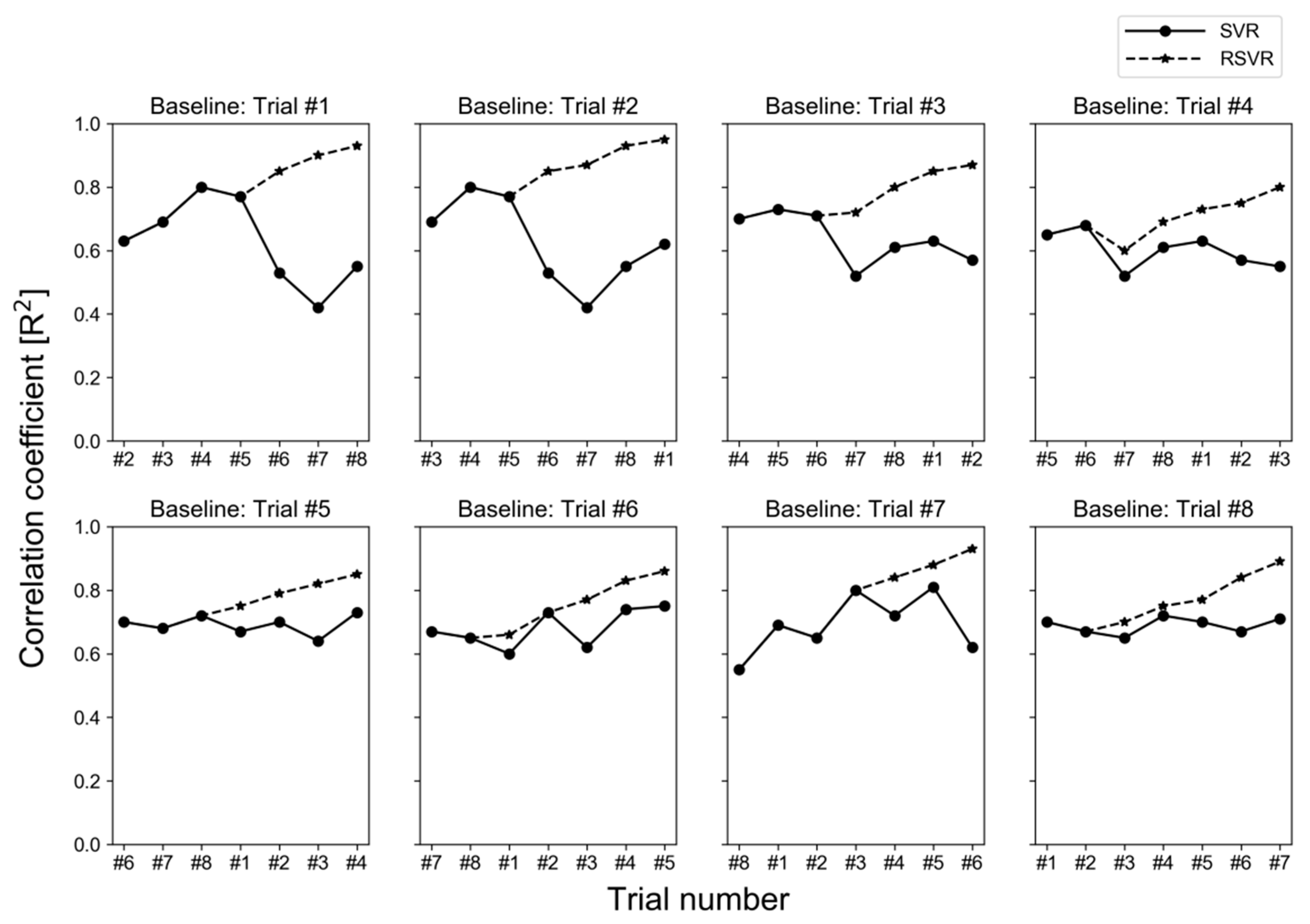
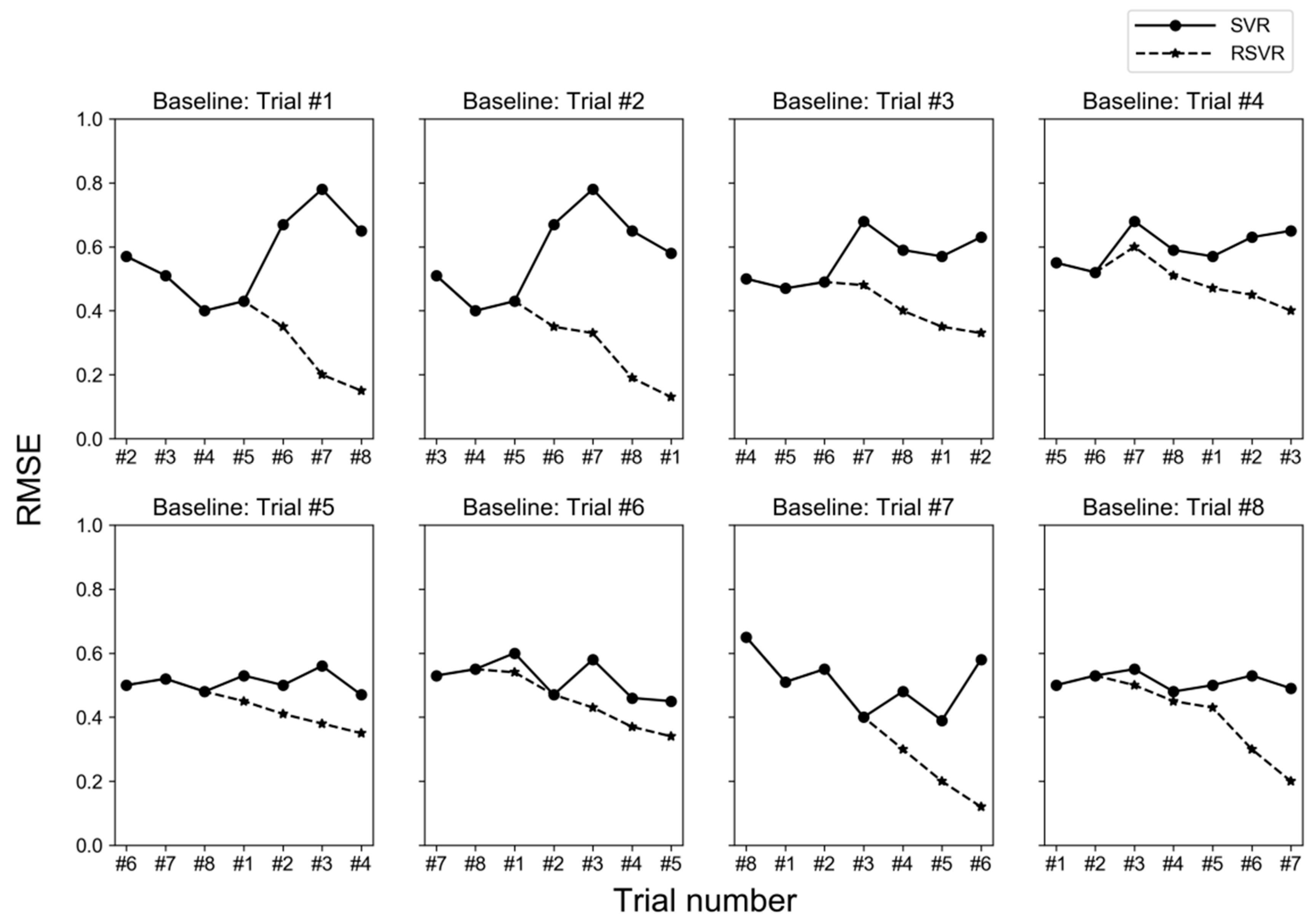
In this study, we used SVR and a new technique proposed in this paper, RSVR, for regression analysis. A comparison of the performance of these techniques was completed using a combination of correlation and RMSE analysis. Figure 2 and Figure 3 illustrate how the values of R2 and RMSE obtained from a single subject respond to additional data, as a representative result of this correlation analysis.
From Figure 2, we note that with the SVR algorithm, the R2 value fluctuates as data from more driving trials are included. For example, when data from trial #1 were the baseline, the correlation coefficient increased from an initial value of 0.63 when considering trial #2, to 0.80 when considering trial #4. However, it subsequently decreased to 0.77, 0.53, and 0.42 when data from trials #5, #6, and #7, were included, respectively. In addition, when data from trials #1, #3, and #4 were the baseline, there was a decrease between the correlation coefficient calculated using only data from the first driving trial (i.e., pre-estimation correlation coefficient), and the value calculated when data from the last driving trial were included (post-estimation). In contrast, with our RSVR method, with trial #1 as the baseline, R2 increased from 0.63, pre-estimation, to 0.87, post-estimation, in spite of the fact that there was a slight decrease in this value when data from trial #5 were first included. Similarly, with trial #2 as the baseline, R2 increased from 0.69 (where trial #3 is the first dataset) to 0.95 (with trial #1 as the final dataset), even though, again, there was a decrease when trial #5 was included. A similar trend is observed when the rest of the datasets (trials #3, #4, #5, #6, #7, and #8) are used as baselines.
Figure 3 shows that the RMSE obtained using SVR fluctuates similarly, when data from more driving trials are included. With trials #1, #2, #3, and #4 as the baselines, the RMSE increased from 0.59 to 0.62, 0.55 to 0.6, 0.54 to 0.63, and 0.59 to 0.63, respectively. In contrast, with the RSVR technique, the RMSE generally decreased with additional driving trials, regardless of the baseline. For example, with trial #1 as the baseline, the RMSE was decreased from an initial value of 0.59 to a final value of 0.20. When trial #2 became the baseline, RMSE again decreased from 0.57 to 0.15. We noted a similar tendency using the rest of trials as a baseline.

3.4. Statistical Analysis of Estimation Methods

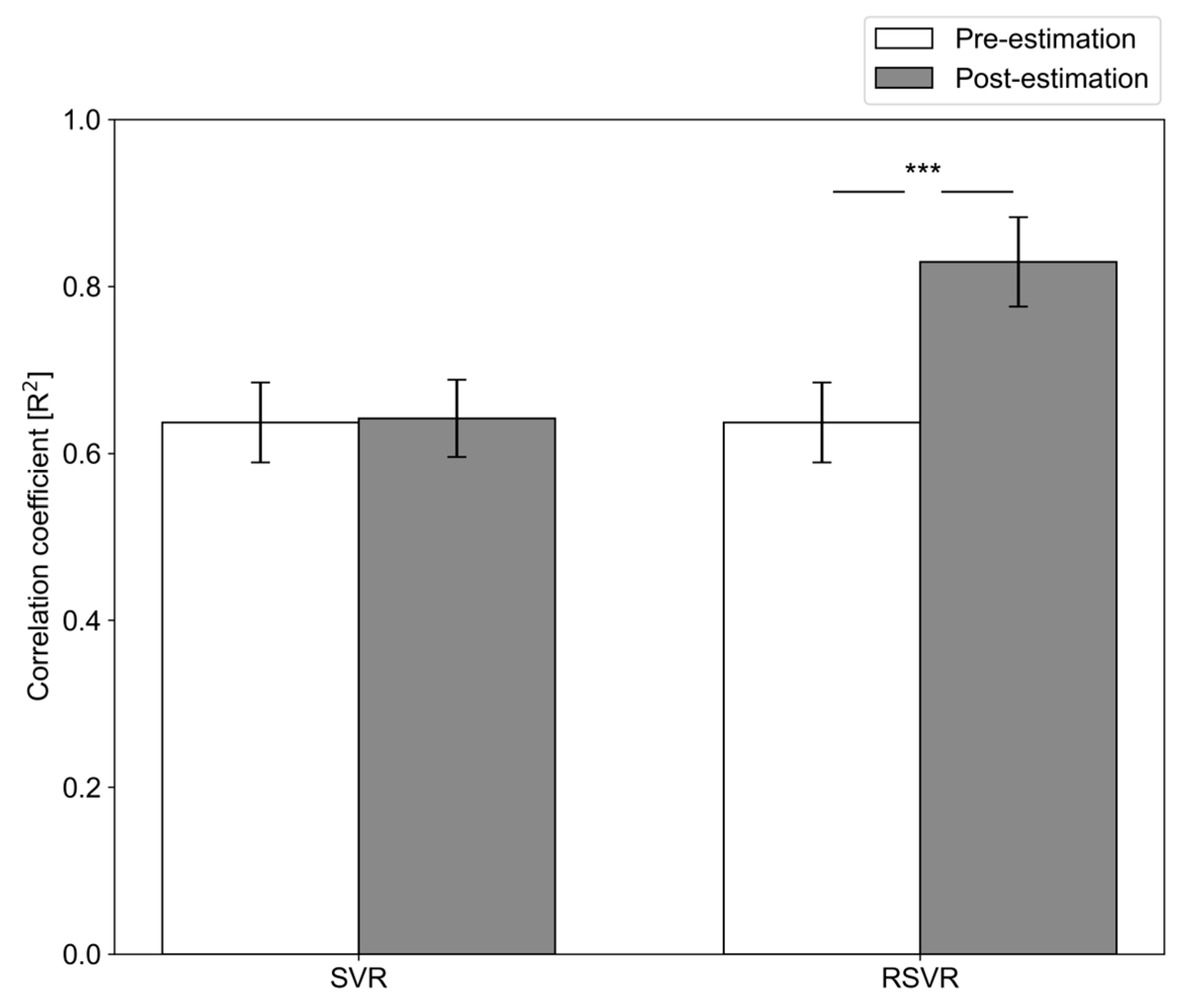
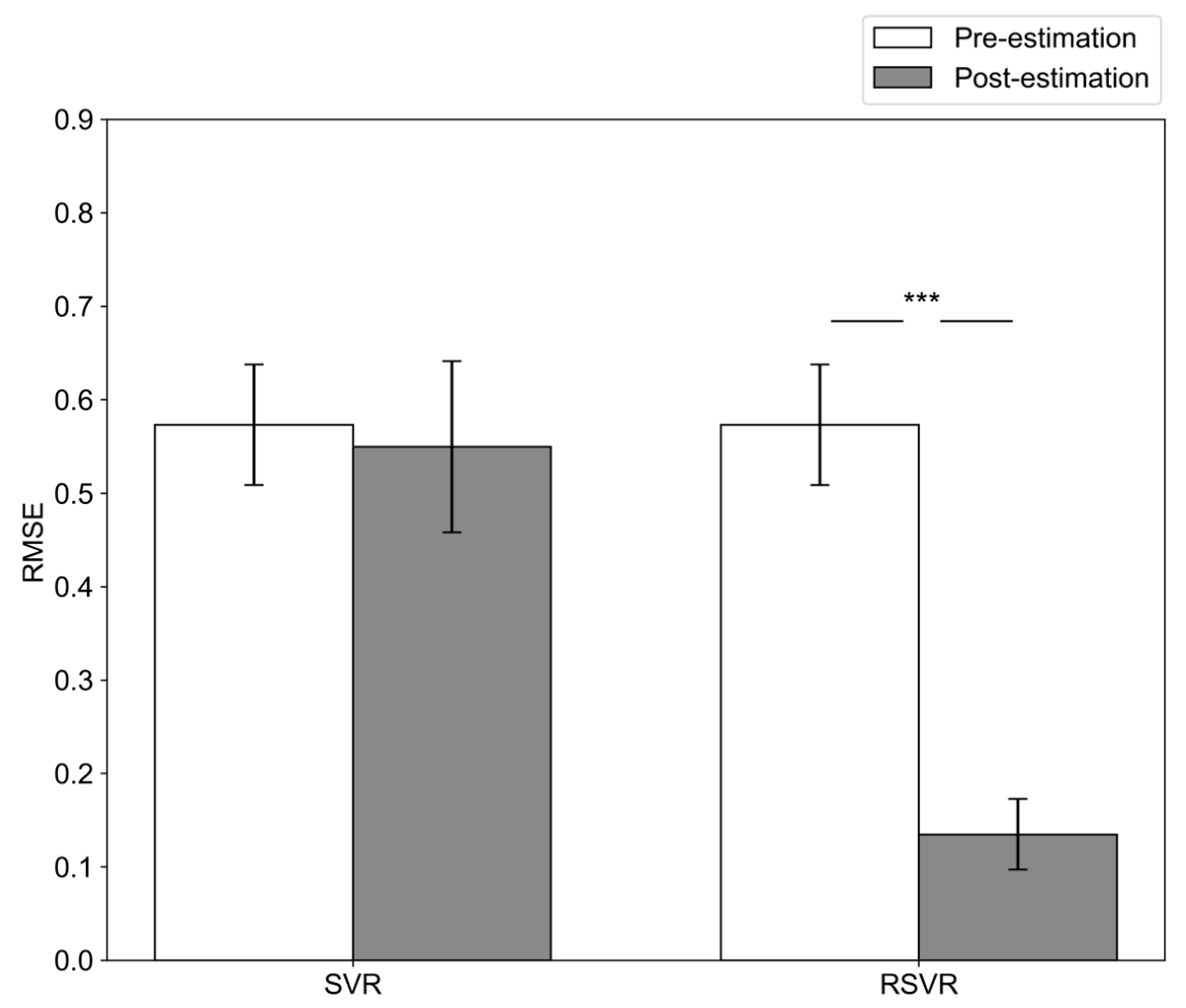
To quantify the change in the performance of the SVR and RSVR techniques and verify their adaptivity to additional driving data, we conducted a Wilcoxon signed-rank test using the pre- and post-estimation R2 and RMSE values obtained from all subjects. The results of this statistical analysis are shown in Figure 4 and Figure 5.
Figure 4 and Figure 5 illustrate that there was no statistically significant (p > 0.05) improvement in the performance of SVR pre- and post-estimation, based on either R2 or RMSE. In contrast, with RSVR, R2 increased from 0.63 ± 0.04 to 0.83 ± 0.06, and RMSE decreased from 0.59 ± 0.08 to 0.15 ± 0.04 (p > 0.05). In addition, with this technique the post-estimation improvements were retained when tested with p < 0.001.

4. Discussion

4.1. Validation of KSS Similarity

As evaluating the drowsiness of the subject through a questionnaire during 50 min of driving could affect the subject’s psychological condition, this study considered evaluating drowsiness after the completion of each trial by watching the footage of the subject’s facial expression recorded during the driving period. However, there was a resting stage before and after each trial to ensure a similar drowsiness perspective during simulated driving and watching the footage video. At this stage, the questions were asked directly to the subject at intervals of 30 s for 5 min (referred to as “direct observation”). After the completion of the trial, the subject was asked to fill the drowsiness questionnaire during the resting and driving periods based on the recorded facial expression (referred to as “indirect observation”). The Wilcoxon signed-rank analysis was performed to analyze the similarity between direct observation KSS and indirect observation KSS. As the results summarized in Table 1 indicate, there was no significant difference between the direct and indirect observation of their drowsiness of the subjects (p-value > 0.05), meaning the subjects were able to recall their drowsiness condition by watching the footage of their facial expression during simulated driving at different times after the completion of the trial.

4.2. Feature Extraction and Selection

Based on results discussed in previous studies, we recorded the absolute power of five common features of EEG signals in the frequency-domain (δ, θ, α, β, and γ). These studies have noted that the absolute power of the α-band correlates well to drowsiness, especially when this signal has been obtained from an occipital site [13,16,25,27]. Because previous studies claimed that α-band, especially from occipital site correlates to drowsiness, we also wanted to check if the results of this study are also similar, as this indicator can ensure the validity of the data collected in this study for drowsiness assessment. We confirmed this observation, as we note that of all the frequency-domain features, the α-band from the O1 occipital site had the best correlation to physiological condition represented by the KSS. As the α-band from the O2 occipital site also showed the second highest correlation, the combined utilization of both occipital sites is considerable. However, we did not employ it together because fewer electrodes and minimal processing are advantageous for feasible implementation in the future. In addition to the powers of the different parameters, we investigated the power-ratios of the frequency bands, since previous studies have noted that the amplitudes of low-frequency EEG bands increase while those of high-frequency bands decrease when a subject is drowsy [16,27]. In particular, employing the β/α and (θ+α)/β power ratios for detecting drowsiness in sleep-deprived subjects has been suggested [25]. We found that both these ratios correlated well with a typical subject’s drowsiness condition, represented by the KSS, confirming this hypothesis. Finally, we observed that, of the time-domain features extracted, only the activity and mobility parameters showed a correlation to drowsiness represented by the KSS. This result validates our previous study, which suggested that activity and mobility parameters could be used to detect drowsiness [13].

4.3. Drowsiness Estimation and RSVR

In previous studies of drowsiness estimation, researchers typically focused on the reliability of EEG signals in classifying two distinct states: awake and drowsy conditions. Garcés Correa et al. employed a time, spectral, and wavelet analysis of EEG signals to estimate these two conditions in a driving environment [28]. From this analysis, they selected six parameters (central frequency, the standard deviation of EEG, first quartile frequency, maximum frequency, and θ and α bands), with which they were able to detect awake conditions up to an accuracy of 87.4%, and drowsy conditions at an accuracy of 83.6%, using an artificial neural network (ANN) classifier. Yeo et al. demonstrated that an SVM classifier could be used to differentiate between alert and drowsy states, based on the spectral features of EEG signals [16]. With this technique, they were able to assess two levels of drowsiness with an accuracy of up to 99.3%. Other studies [13,16] have attempted to classify drowsiness using three levels: An awake condition; a strong drowsy condition; and a weak drowsy condition, which can be considered to be the transition stage between the binary awake and drowsy conditions, as detecting this weak drowsy condition enables early assessment of drowsiness. However, all these studies focused only on detecting drowsiness by using a relatively big dataset and divided into such portion to train and test. In addition, previous studies did not consider improving the estimation performance as the subject trial increases.
The key idea in this study was to investigate whether EEG parameters can be used as a predictor for a subjective drowsiness evaluation score, using a model trained with a limited dataset. In addition, this model should be able to improve its estimation performance automatically as more data are acquired. Thus, in this study we used a limited dataset to train our RSVR model. Then, as additional trial data were included, the RSVR model estimated the drowsiness condition characterized by these data, and automatically decided if the result was sufficiently accurate and whether to include the trial data as additional training data. Since the RSVR only chooses data that lead to a high R2 value and a low RMSE as additional training data, its estimation performance can be improved. The combination of initial and additional data is then used for building a new RSVR model to estimate drowsiness for the next set of trial data.
The concept of recurrence in RSVR refers to the use of the output of estimation as the input for building the next regression model. In spite of its use of actual drowsiness conditions as the initial training data, the RSVR uses model estimates as additional training data. This is in consideration of ease of use, as it is not convenient for a system to prompt the subject to assess their drowsiness every time a new activity occurs. Thus, by using the estimate from a previous trial as training data, operation of the model is made more convenient. In spite of this design, Figure 2 and Figure 3 show that, in general, including more driving trial data increases the value of R2 obtained with RSVR, and decreases the RMSE, regardless of the initial baseline. Although both the R2 and RMSE values sometimes fluctuated, the overall results were better than those obtained with SVR. This indicates that the RSVR algorithm can predict subjectively assessed drowsiness.
Another consideration is early drowsiness detection, which in some previous studies has been enabled by classifying drowsiness into three categories [13,16]. However, while this is better than binary classification, three conditions are still not enough for accident prevention, where drowsiness should be detected as early as possible to prevent accidents. Once the earliest state of drowsiness has been detected, the ideal system is able to give an early warning to the subject, allowing them to take preventive action to avoid accidents. Since drowsiness changes gradually over time, it is possible to detect its earliest state, which occurs before the transition stage defined for three-level drowsiness classification systems. To accommodate this, more detailed categories are needed as markers for early drowsiness states. Thus, in this study, we employed a nine-level drowsiness evaluator, with categories ranging from very alert to very sleepy, as defined by the KSS.
Our statistical analysis shows that, with standard SVR, there is no significant difference in the R2 and RMSE values obtained pre-estimation and post-estimation (Figure 4 and Figure 5). In contrast, with RSVR, there was a statistically significant (p < 0.001) increase in R2, from 0.63 to 0.83, and a statistically significant (p < 0.001) decrease in RMSE, from 0.59 to 0.15. A previous study showed that drowsiness estimates obtained by relating SVR to physiological parameters had R2 and RMSE values of up to 0.69 and 0.27, respectively [18]. The studies listed in Table 3, that used adaptive ANN (AdANN) and multinomial logistic regression (MLR) methods to estimate drowsiness, obtained RMSEs of 0.96 and 0.25, respectively [29,30]. Based on these results, our RSVR method outperforms the standard SVR technique, and ANN and MLR methods as implemented in previous studies.
While the techniques presented in this paper have demonstrated potential for estimating drowsiness, some limitations need to be considered. At present, we use a self-assessed questionnaire to evaluate the trial participants’ drowsiness condition, which raises issues regarding the subjective drowsiness perspective recorded [31]. However, as this questionnaire is widely used in other studies, it is difficult to conclude that it is not reliable in evaluating drowsiness [15,16,30]. Other possible limitations relate to the subject and research environment where tests were performed. In this study, sixteen male subjects were selected for participation. While this may seem to be a small number, many studies in the drowsiness estimation research field have used similarly small populations of 10–20 subjects [18,32,33,34,35]. Moreover, as this study focuses on intra-subject optimization, the number of subjects does not affect the quality of the model. Although the experiments were conducted in a driving simulator environment, the findings of this study are not solely applicable to drowsy driving problems; we selected the specific research environment and settings because the monotony of the driving task induces drowsiness easily. Further, we employed young male volunteers only in this study. As mentioned above, we believe that the model quality is not affected by this issue. However, we should conduct this experiment with middle-aged or elderly and female participants in the future, for consideration of a more representative demographic.

5. Conclusions

In this study, we investigated the feasibility of estimating drowsiness from EEG parameters. To model an actual scenario, we trained our technique with a limited dataset, and gradually increased the quantity of data as the subject’s activity increased. In spite of the limited training data initially provided, the proposed method was still able to improve its drowsiness estimation performance as more of a subject’s activity was considered. Using five physiological parameters extracted from O1 electrode site (the absolute power of α, the β/α and (θ+α)/β ratios, and activity and mobility) and a custom regression method (RSVR), we were able to estimate drowsiness with R2 and RMSE values up to 0.83 and 0.15, respectively. Even though our experiments were conducted in a driving environment, the technique suggested can be adapted for other purposes and is not limited to driving activity. In addition, our technique classifies drowsiness in nine levels represented by the KSS, in contrast to the two- and three-level classifications typically used.

Author Contributions

The conceptualization was developed by I.A.A. and T.I.; the methodology was developed by I.A.A.; the software was coded by I.A.A.; the validation was reviewed by T.I.; the formal analysis and data curation were conducted by I.A.A.; the writing-original draft preparation was conducted by I.A.A.; the writing-review was reviewed by T.I.; The visualization was provided by I.A.A.; the supervision, project administration, and funding acquisition were conducted by T.I.

Funding

This research was partially supported by JSPS KAKENHI JP16K00375.

Acknowledgments

The authors would like to express their gratitude to Takamasa Morie, Mitaku Utsunomiya, and Arthur Mourits Rumagit for their cooperation in this study.

Conflicts of Interest

The authors declare no conflict of interest.

References

  1. Abtahi, S.; Hariri, B.; Shirmohammadi, S. Driver drowsiness monitoring based on yawning detection. In Proceedings of the 2011 IEEE International Instrumentation and Measurement Technology Conference, Binjiang, China, 10–12 May 2011; pp. 1–4. [Google Scholar]
  2. Morris, D.M.; Pilcher, J.J.; Switzer III, F.S. Lane heading difference: An innovative model for drowsy driving detection using retrospective analysis around curves. Accid. Anal. Prev. 2015, 80, 117–124. [Google Scholar] [CrossRef] [PubMed]
  3. Sandström, M.; Lampsijärvi, E.; Holmström, A.; Maconi, G.; Ahmadzai, S.; Meriläinen, A.; Hæggström, E.; Forsman, P. Detecting lane departures from steering wheel signal. Accid. Anal. Prev. 2017, 99, 272–278. [Google Scholar] [CrossRef]
  4. Patel, M.; Lal, S.K.L.; Kavanagh, D.; Rossiter, P. Applying neural network analysis on heart rate variability data to assess driver fatigue. Expert Syst. Appl. 2011, 38, 7235–7242. [Google Scholar] [CrossRef]
  5. Sahayadhas, A.; Sundaraj, K.; Murugappan, M.; Palaniappan, R. Physiological signal based detection of driver hypovigilance using higher order spectra. Expert Syst. Appl. 2015, 42, 8669–8677. [Google Scholar] [CrossRef]
  6. Piotrowski, Z.; Szypulska, M. Classification of falling asleep states using HRV analysis. Biocybern. Biomed. Eng. 2017, 37, 290–301. [Google Scholar] [CrossRef]
  7. Hu, S.; Zheng, G. Driver drowsiness detection with eyelid related parameters by Support Vector Machine. Expert Syst. Appl. 2009, 36, 7651–7658. [Google Scholar] [CrossRef]
  8. Ma’touq, J.; Al-Nabulsi, J.; Al-Kazwini, A.; Baniyassien, A.; Al-Haj Issa, G.; Mohammad, H. Eye blinking-based method for detecting driver drowsiness. J. Med. Eng. Technol. 2014, 38, 416–419. [Google Scholar] [CrossRef]
  9. Jackson, M.L.; Kennedy, G.A.; Clarke, C.; Gullo, M.; Swann, P.; Downey, L.A.; Hayley, A.C.; Pierce, R.J.; Howard, M.E. The utility of automated measures of ocular metrics for detecting driver drowsiness during extended wakefulness. Accid. Anal. Prev. 2016, 87, 127–133. [Google Scholar] [CrossRef]
  10. Lee, B.G.; Lee, B.L.; Chung, W.Y. Mobile healthcare for automatic driving sleep-onset detection using wavelet-based EEG and respiration signals. Sensors 2014, 14, 17915–17936. [Google Scholar] [CrossRef]
  11. Igasaki, T.; Nagasawa, K.; Murayama, N.; Hu, Z. Drowsiness estimation under driving environment by heart rate variability and/or breathing rate variability with logistic regression analysis. In Proceedings of the 2015 8th International Conference on Biomedical Engineering and Informatics (BMEI), Shenyang, China, 14–16 October 2015; pp. 189–193. [Google Scholar]
  12. Balasubramanian, V.; Adalarasu, K. EMG-based analysis of change in muscle activity during simulated driving. J. Bodyw. Mov. Ther. 2007, 11, 151–158. [Google Scholar] [CrossRef]
  13. Akbar, I.A.; Rumagit, A.M.; Utsunomiya, M.; Morie, T.; Igasaki, T. Three drowsiness categories assessment by electroencephalogram in driving simulator environment. In Proceedings of the 2017 39th Annual International Conference of the IEEE Engineering in Medicine and Biology Society (EMBC), Seogwipo, South Korea, 11–15 July 2017; pp. 2904–2907. [Google Scholar]
  14. Chen, L.; Zhao, Y.; Zhang, J.; Zou, J. Automatic detection of alertness/drowsiness from physiological signals using wavelet-based nonlinear features and machine learning. Expert Syst. Appl. 2015, 42, 7344–7355. [Google Scholar] [CrossRef]
  15. Kaida, K.; Takahashi, M.; Åkerstedt, T.; Nakata, A.; Otsuka, Y.; Haratani, T.; Fukasawa, K. Validation of the Karolinska sleepiness scale against performance and EEG variables. Clin. Neurophysiol. 2006, 117, 1574–1581. [Google Scholar] [CrossRef] [PubMed]
  16. Yeo, M.V.M.; Li, X.; Shen, K.; Wilder-Smith, E.P.V. Can SVM be used for automatic EEG detection of drowsiness during car driving? Saf. Sci. 2009, 47, 115–124. [Google Scholar] [CrossRef]
  17. Dijk, D.J.; Lockley, S.W. Integration of human sleep-wake regulation and circadian rhythmicity. J. Appl. Physiol. 2002, 92, 852–862. [Google Scholar] [CrossRef] [PubMed]
  18. Lin, C.T.; Chuang, C.H.; Huang, C.S.; Tsai, S.F.; Lu, S.W.; Chen, Y.H.; Ko, L.W. Wireless and wearable EEG system for evaluating driver vigilance. IEEE Trans. Biomed. Circuits Syst. 2014, 8, 165–176. [Google Scholar]
  19. Maia, Q.; Grandner, M.A.; Findley, J.; Gurubhagavatula, I. Short and long sleep duration and risk of drowsy driving and the role of subjective sleep insufficiency. Accid. Anal. Prev. 2013, 59, 618–622. [Google Scholar] [CrossRef] [PubMed] [Green Version]
  20. Aidman, E.; Johnson, K.; Paech, G.M.; Della Vedova, C.; Pajcin, M.; Grant, C.; Kamimori, G.; Mitchelson, E.; Hoggan, B.L.; Fidock, J.; et al. Caffeine reduces the impact of drowsiness on driving errors. Transp. Res. Part F Traffic Psychol. Behav. 2018, 54, 236–247. [Google Scholar] [CrossRef]
  21. Soldatos, C.R.; Kales, J.D.; Scharf, M.B.; Bixler, E.O.; Kales, A. Cigarette smoking associated with sleep difficulty. Science 1980, 207, 551–553. [Google Scholar] [CrossRef]
  22. Hjorth, B. EEG analysis based on time domain properties. Electroencephalogr. Clin. Neurophysiol. 1970, 29, 306–310. [Google Scholar] [CrossRef]
  23. Oh, S.-H.; Lee, Y.-R.; Kim, H.-N. A Novel EEG Feature Extraction Method Using Hjorth Parameter. Int. J. Electron. Electr. Eng. 2014, 2, 106–110. [Google Scholar] [CrossRef]
  24. Vidaurre, C.; Krämer, N.; Blankertz, B.; Schlögl, A. Time Domain Parameters as a feature for EEG-based Brain–Computer Interfaces. Neural Networks 2009, 22, 1313–1319. [Google Scholar] [CrossRef] [PubMed]
  25. Eoh, H.J.; Chung, M.K.; Kim, S.H. Electroencephalographic study of drowsiness in simulated driving with sleep deprivation. Int. J. Ind. Ergon. 2005, 35, 307–320. [Google Scholar] [CrossRef]
  26. Pedregosa, F.; Varoquaux, G.; Gramfort, A.; Michel, V.; Thirion, B.; Grisel, O.; Blondel, M.; Prettenhofer, P.; Weiss, R.; Dubourg, V.; et al. Scikit-learn: Machine Learning in Python. J. Mach. Learn. Res. 2011, 12, 2825–2830. [Google Scholar]
  27. Awais, M.; Badruddin, N.; Drieberg, M. A Hybrid Approach to Detect Driver Drowsiness Utilizing Physiological Signals to Improve System Performance and Wearability. Sensors 2017, 17, 1991. [Google Scholar] [CrossRef] [PubMed]
  28. Garcés Correa, A.; Orosco, L.; Laciar, E. Automatic detection of drowsiness in EEG records based on multimodal analysis. Med. Eng. Phys. 2014, 36, 244–249. [Google Scholar] [CrossRef]
  29. Jacobé de Naurois, C.; Bourdin, C.; Bougard, C.; Vercher, J.L. Adapting artificial neural networks to a specific driver enhances detection and prediction of drowsiness. Accid. Anal. Prev. 2018, 121, 118–128. [Google Scholar] [CrossRef]
  30. Murata, A.; Fujii, Y.; Naitoh, K. Multinomial Logistic Regression Model for Predicting Driver’s Drowsiness Using Behavioral Measures. Procedia Manuf. 2015, 3, 2426–2433. [Google Scholar] [CrossRef]
  31. Friedrichs, F.; Yang, B. Drowsiness monitoring by steering and lane data based features under real driving conditions. In Proceedings of the 2010 18th European Signal Processing Conference, Aalborg, Denmark, 23–27 August 2010; pp. 209–213. [Google Scholar]
  32. Li, G.; Lee, B.; Chung, W. Smartwatch-Based Wearable EEG System for Driver Drowsiness Detection. IEEE Sens. J. 2015, 15, 7169–7180. [Google Scholar] [CrossRef]
  33. Zhang, Z.; Luo, D.; Rasim, Y.; Li, Y.; Meng, G.; Xu, J.; Wang, C. A Vehicle Active Safety Model: Vehicle Speed Control Based on Driver Vigilance Detection Using Wearable EEG and Sparse Representation. Sensors 2016, 16, 242. [Google Scholar] [CrossRef]
  34. Zhang, X.; Li, J.; Liu, Y.; Zhang, Z.; Wang, Z.; Luo, D.; Zhou, X.; Zhu, M.; Salman, W.; Hu, G.; et al. Design of a Fatigue Detection System for High-Speed Trains Based on Driver Vigilance Using a Wireless Wearable EEG. Sensors 2017, 17, 486. [Google Scholar] [CrossRef]
  35. Larue, G.S.; Rakotonirainy, A.; Pettitt, A.N. Driving performance impairments due to hypovigilance on monotonous roads. Accid. Anal. Prev. 2011, 43, 2037–2046. [Google Scholar] [CrossRef] [PubMed] [Green Version]
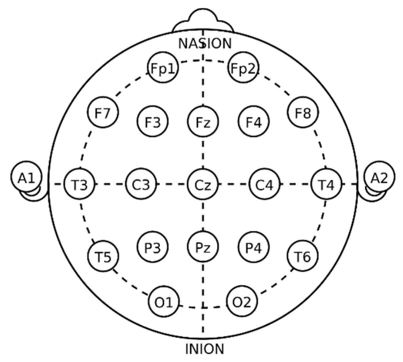
Figure 1. Electroencephalogram (EEG) electrode placement according to the international 10–20 system.
Information 10 00217 g001
Figure 2. Comparison of the correlation between KSS score, and support vector regression (SVR) and recurrent SVR (RSVR) estimates for subject #16, with different driving trials used as baselines.
Information 10 00217 g002
Figure 3. Comparison of the RMSE of subject #16’s SVR and RSVR estimates with different driving trials used as baselines.
Information 10 00217 g003
Figure 4. Statistical analysis of the correlation coefficients of pre- and post-trial estimation performed using SVR (without proposed method) and RSVR (with proposed method) (***: p < 0.001, **: p < 0.01, *: p < 0.05).
Information 10 00217 g004
Figure 5. Statistical analysis of the RMSE of pre- and post-trial estimation performed using SVR (without proposed method) and RSVR (with proposed method) (***: p < 0.001, **: p < 0.01, *: p < 0.05).
Information 10 00217 g005
Table 1. Validation of similarity between KSS evaluated from direct and indirect observation.
SubjectPre-Driving TaskPost-Driving Task
Direct ObservationIndirect ObservationDirect ObservationIndirect Observation
#15.4 ± 0.95.4 ± 0.9 NS6.3 ± 0.66.3 ± 0.6 NS
#23.6 ± 0.43.6 ± 0.4 NS6.1 ± 0.56.1 ± 0.5 NS
#34.6 ± 2.64.6 ± 2.5 NS6.8 ± 2.26.7 ± 2.2 NS
#46.4 ± 1.96.4 ± 1.8 NS7.8 ± 1.07.8 ± 1.1 NS
#54.8 ± 2.44.8 ± 2.4 NS8.1 ± 1.28.0 ± 1.3 NS
#63.6 ± 2.53.6 ± 2.5 NS7.1 ± 0.97.1 ± 0.9 NS
#76.0 ± 2.06.0 ± 2.0 NS7.3 ± 1.57.3 ± 1.5 NS
#84.3 ± 2.24.2 ± 2.2 NS6.0 ± 2.46.0 ± 2.4 NS
#96.0 ± 2.06.0 ± 2.0 NS7.2 ± 0.97.1 ± 0.9 NS
#103.5 ± 0.43.5 ± 0.4 NS6.3 ± 0.96.3 ± 0.8 NS
#114.0 ± 1.44.0 ± 1.4 NS6.3 ± 1.66.3 ± 1.6 NS
#123.8 ± 1.13.8 ± 1.2 NS5.4 ± 0.75.3 ± 0.7 NS
#133.4 ± 0.33.4 ± 0.3 NS5.2 ± 2.95.2 ± 2.9 NS
#144.2 ± 0.74.2 ± 0.7 NS5.9 ± 0.75.9 ± 0.7 NS
#154.1 ± 1.24.1 ± 1.2 NS6.4 ± 0.76.4 ± 0.7 NS
#162.0 ± 0.82.0 ± 0.8 NS5.9 ± 0.65.9 ± 0.6 NS
NS: No-significance vs. direct observation (p > 0.05). All values are expressed as mean ± SD.
Table 2. Analysis of correlation between each parameter, and drowsiness condition represented by KSS (Karolinska sleepiness scale) for all electrode sites. Act: Activity, Mob: Mobility, Com: Complexity.
Electrode NameCorrelation Coefficient (R2)
δθαβγβ/α(θ + α)/βAct.Mob.Com.
Fp10.040.130.140.220.190.010.060.150.100.05
Fp20.120.130.270.240.210.020.070.120.030.05
F30.100.110.100.200.160.070.100.090.000.01
F40.020.050.090.250.210.060.090.110.090.13
F70.100.110.100.190.160.020.100.120.040.01
F80.120.070.060.240.200.030.070.090.010.02
Fz0.130.170.040.240.190.030.040.130.070.01
C30.170.100.190.120.190.120.180.200.090.08
C40.150.100.200.150.180.200.220.310.110.09
Cz0.170.080.300.140.190.300.220.310.180.09
P30.120.200.500.140.200.540.420.520.430.15
P40.100.160.460.130.190.460.380.480.330.17
Pz0.150.200.600.130.190.610.600.530.490.15
O10.180.180.850.170.200.760.740.700.690.18
O20.180.170.750.160.210.640.720.640.590.18
T30.150.060.290.150.240.300.230.220.090.08
T40.130.060.280.150.220.230.240.210.120.09
T50.150.180.360.140.200.230.300.400.310.01
T60.140.170.370.150.220.250.310.360.300.01
Table 3. Comparison of previous studies and the current study in drowsiness estimation.
Estimation MethodDrowsiness CategoriesRMSE
Jacobé et al. [29]AdANN50.96
Murata et al. [30]MLR30.25
This studyRSVR90.15