Multi-Sensor Activity Monitoring: Combination of Models with Class-Specific Voting

Abstract

This paper presents a multi-sensor model combination system with class-specific voting for physical activity monitoring, which combines multiple classifiers obtained by splicing sensor data from different nodes into new data frames to improve the diversity of model inputs. Data obtained from a wearable multi-sensor wireless integrated measurement system (WIMS) consisting of two accelerometers and one ventilation sensor have been analysed to identify 10 different activity types of varying intensities performed by 110 voluntary participants. It is noted that each classifier shows better performance on some specific activity classes. Through class-specific weighted majority voting, the recognition accuracy of 10 PA types has been improved from 86% to 92% compared with the non-combination approach. Furthermore, the combination method has shown to be effective in reducing the subject-to-subject variability (standard deviation of recognition accuracies across subjects) in activity recognition and has better performance in monitoring physical activities of varying intensities than traditional homogeneous classifiers.

1. Introduction

Physical activity (PA) is any bodily movement worked by skeletal muscles that requires more energy expenditure than resting [1], such as walking, running, swimming, or aerobic exercise and strength training. Getting proper physical activity throughout the day can lower the risk of type 2 diabetes, cardiovascular disease, stroke, and obesity. However, most people do not do enough physical activity, because it is not easy to be measured. Therefore, accurate tracking and monitoring of PA under free-living conditions is of significant importance to cultivate scientific living habits and improve an individual’s health.

The target of PA monitoring is oriented to recognize the type of activity, duration of time, and the intensity of daily activities in real-time. By estimating the energy consumption, it provides important guidance for people’s scientific fitness. Accelerometer-based PA monitoring has become a popular and handy choice recently due to its low subject burden and non-invasive nature. Hendelman et al. have demonstrated the correlations between accelerometer counts and energy expenditure [2]. Scanaill et al. highlighted that the wearable telemonitoring system has provided a mechanism of assessing health status in the living environment [3]. However, a single accelerometer cannot accurately represent activities that produce similar acceleration profiles but have different energy expenditures [4]. For example, walking at a certain speed may result in acceleration outputs similar to that of walking at the same speed while carrying a load, but the energy expenditure is very different. To address the drawbacks of this method, researchers have investigated alternative techniques. Shoaib et al. placed multiple sensors (accelerometer, gyroscope, and linear acceleration sensor) on different parts of the body for human activity recognition [5]. Ermes et al. have extracted signal features from three-axis accelerometers on the hip, wrist, and GPS signal [6]. To investigated advanced computational techniques, machine learning and sensor fusion are applied to differentiate the activity patterns [7]. Altini et al. have fused data from five sensor units to estimate the energy consumption of various activities with different intensities [8]. A multi-sensor integrated measurement system was developed with two three-axial accelerometers and a ventilation sensor to monitor and measure physical activities [9].

Machine learning is the technology where existing knowledge is reorganized to improve its own performance continuously [10]. Some methods based on machine learning have been utilized to recognize physical activity patterns. The hidden Markov model (HMM) and artificial neural network (ANN) have been typically employed to estimate the type of PA [4,11,12]. Support Vector Machines (SVMs) have been used for medical and biomedical assessment due to its powerful classification and estimation capabilities [13,14,15]. A single SVM classifier has also been utilized for PA recognition based on a multi-sensor system [16]. Considering that even for the same activity, there will be differences among different people, it is not easy to characterize the diversities between subjects by a single classifier. In order to improve the generalization ability of machine learning, ensemble learning, which combines multiple classifiers to achieve a better predictive capacity, is proposed and applied in pattern recognition [17,18]. Zheng et al. ensembled the models based on the different temporal scales and statistic features of an accelerometer [19]. Ravi et al. combined multiple different classifiers using plurality voting for activity recognition from a single accelerometer [20]. In addition, different sensor nodes or different types of sensors can establish heterogeneous classification models. Kaur et al. achieved sustainable results on a set of common activities through ensemble learning [21]. Since sensor nodes in different parts can acquire different statistics of movement, the multi-sensor measurement system has the potential to achieve better performance in the identification of PA type than a homogeneous classifier. Some preliminary research on the majority voting-based ensemble learning has been carried out for PA monitoring. The conventional weight-based ensemble method typically treated the outputs of the same base classifier with the same weight. Mo et al. have ensembled multiple classifiers with conventional weighted voting to improve the accuracy of the identification of six PA types [22]. Considering that the combination of different sensors and classifiers may acquire different performances in recognizing different PA patterns, increasing the diversity of model inputs and differentiating the weights of the different types of activity classifiers may make a direct impact on the classification ability of the models.

In this paper, a multi-sensor activity monitoring system proposed for PA tracking and pattern recognition has been analyzed in detail, gathering multiple classifiers that support the vector machine algorithm corresponding to different combinations of sensor nodes data. Taking into consideration that the accuracy of classifying distinct PA types has been reflected within different types of classifiers, the Class-specific Weighted Majority Voting (CWMV) has been presented for the model combination. In order to verify the idea of this paper, the experiments of classification by using different classifier integration methods have been conducted. The data on the performance of 110 participants’ activity have been evaluated and recorded by both model combination and non-combination. Moreover, the comparison between the CWMV and the plurality majority voting for the multi-sensor model combination system are also explored and analyzed.

2. Model Combination Method

In machine learning, an ensemble learning method combines multiple classifiers to obtain a better predictive performance than that obtained by any of the constituent classifiers [17,23,24], and it is a technique that usually combines a number of weak classifiers together to produce a strong classifier. Empirically, the model combination classifier tends to yield better results when a significant diversity among the classifiers exists [18,25]. Many model combination methods, therefore, seek to promote diversity among the classifiers by using different resampling technologies, such as bagging [26], boosting [27], and Ada-boost [28]. Another approach to achieve diversity is to use different training parameters for different classifiers or to use a variety of strong learning algorithms [29]. For multi-sensor measurement systems, different sensors would have different statistical distributions. Therefore, with the multi-sensor model combination, the model can be designed with better generalization ability than a single multi-input model. By choosing different sensors, it is easier to realize the diversity of the classifier datasets than traditional approaches. Moreover, the model combination as an application of ensemble learning is also a good choice for realizing multi-sensor data fusion.

2.1. Model Combination System Design

The overall architecture of the multi-sensor model combination system with CWMV is given in Figure 1 below. The data sets used for the following model combination step were collected by combining the dataflow of different sensor nodes of the multi-sensor measurement system. Furthermore, the activity recognition features that are relevant to these sensor combination datasets have been extracted and selected. By selecting sensor nodes and feature combinations, classifiers of different feature sets could be derived from each sensor data set. The diversity of the base classifiers could be achieved as well. As for each base classifier, a machine-learning model was selected and trained. The partially independent data set was divided as a testing dataset to validate the performance of every single base classifier. Under these conditions, each classifier had its own results for PA recognition. At length, the final classification decision was obtained through fusing the classification results from all the base classifiers, especially with a class-specific weighted majority voting.

2.2. Class-Specific Weighted Majority Voting

Combining strategy refers to the voting method/scheme where different classifiers are combined based on their different sensors to obtain better predictive performance. It is another important consideration of any model combination system in addition to the diversity of the classifiers. Several different model combination strategies have been studied for the model combination system, such as plurality majority voting, weighted majority voting, and stacking [30]. Specifically, weighted majority voting is a popular classifier combination method for ensemble learning, which assigns different voting weights to the different classifiers with different accuracies. By doing so, it generally achieves better results than plurality voting. However, since the classifiers based on the different sensor sets usually have different recognition accuracies of the different PA types, it is not reasonable to assign a consistent weight for each classifier. Therefore, a class-specific weighted majority voting is presented in this study for the multi-sensor model combination system.

Defining a subject space {S_j|S_j ∈ S, 1 ≤ j ≤ N} and multiple base classifiers {C_t|C_t ∈ C, 1 ≤ t ≤ T}, d_t,j which represents the decision of the tth classifier C_t on a subject S_j can be described as:

$$d_{t,j}=\{\begin{array}{l}1, \mathrm{if} C_t \mathrm{votes} S_j\\ 0, \mathrm{if} C_t \mathrm{votes} \mathrm{others}\end{array}$$

(1)

Further, assuming that there is a way of estimating the identification performance of each classifier, and that weight w_t is assigned to the classifier C_t in proportion to its accuracy, then, the total weighted voting scores g_j of subject S_j can be calculated as:

$$g_j={\displaystyle \sum _{t=1}^T{w}_t{d}_{t,j}}$$

(2)

where T is the number of classifiers. Among all the subject space S, the one which gets the maximum voting scores is the final voting subject S_vote. It can be described as:

$$S_{vote}=S_J, \mathrm{when} J=\underset{j}{\arg \max }(g_j)$$

(3)

Or

$$S_{vote}=S_J, \mathrm{when} {\displaystyle \sum _{t=1}^T{w}_t{d}_{t,J}}=\underset{j=1}{\overset{N}{\max }}{\displaystyle \sum _{t=1}^T{w}_t{d}_{t,j}}$$

(4)

where the function argmax returns an integer J, which stands for the index of the maximum voting scores. Equations (3) and (4) is the normal weighted majority voting being wildly used [31]. Every classifier has a different voting weight according to its identification accuracy. However, for the multi-sensor system, different classifiers have different accuracies on the different PA types. For example, a classifier based on the sensor dataset of a single wrist accelerometer has better identification accuracy on the computer work than the treadmill exercise. For this reason, in the process of voting, weighing the decisions of the classifier with different confidence on different PA types may further improve the overall performance than that obtained by normal weighted majority voting with the same weight for the same classifier on different PA type recognition. Through the training and testing, the weight w_t,j of classifier C_t in proportion to its estimated performance on the different subjects j (different PA types) can be obtained. The weight w_t,j can be defined as:

$$w_{t,j}=getPresicion(C_t \mathrm{on} S_j)$$

(5)

The function getPrecision returns the precision of a classifier on a specific subject. The precision of the model is derived from the confusion matrix, which can be described as:

$$Precision=\frac{TP}{TP+FP}$$

(6)

where the TP is the true positive and the FP is the false positive [32]. Then, the total voting scores g_j of subject S_j can be calculated as:

$$g_j={\displaystyle \sum _{t=1}^T{w}_{t,j}{d}_{t,j}}$$

(7)

The final voted subject S_vote can be calculated as:

$$S_{vote}=S_J, \mathrm{when} J=\underset{j}{\arg \max }{\displaystyle \sum _{t=1}^T{w}_{t,j}{d}_{t,j}}$$

(8)

This class-specific weighted majority voting is more reasonable than the normal weighted majority voting for the model combination system. It considers the different identification accuracies of the different classifiers (based on the different sensor sets) on the different PA types.

3. Multi-Sensor Measurement Platform

3.1. Multi-Sensor Monitoring System Based on the WIMS

The multi-sensor wireless integrated measurement system (WIMS) is designed to assess human physical activity. Figure 2 illustrates the overall architecture of the multi-sensor activity monitoring system. By attaching multiple sensors to the human body, physical activity signals corresponding to different parts of the human body can be obtained. Feature extraction and selection are then performed. Through certain machine learning algorithms, the physical activity patterns are identified and the fitness of the body is evaluated. Based on the assessment results, expert guidance and suggestions can be provided to people to improve their health and fitness.

3.2. WIMS System Design and Realization

The sensor locations of the WIMS were selected according to the survey on the wearable sensor convenience [13]. As a result, the two accelerometers are attached to the hip and wrist respectively, while the ventilation sensor is attached around the abdomen. For free-living acceptance, the WIMS is designed with wireless capability, low burden, extended battery life, easy operation, and sufficient data storage [33]. The WIMS measures the body motion and respiration of a human subject, and the collected data are subsequently fused to determine the PA types and quantify the PA-related energy expenditure. Specifically, three sensor units are included in the WIMS:

• Hip Unit: one tri-axial accelerometer ADXL345 worn at the hip, to measure the body motions that characterize the degree of PA of the lower part of the body;
• Wrist Unit: one tri-axial accelerometer ADXL345 worn on the wrist, to measure the arm and hand motions that characterize the PA of the upper part of the body;
• Abdominal Unit: one ventilation sensor made of piezoelectric crystal wrapped around the abdomen, for measuring the expansion and contraction resulting from the subject’s respiration (breathing rate and volume).

Figure 3 illustrates the hardware configuration of the WIMS. All the sensor units have embedded ZigBee and MCU modules. The wrist unit and the abdominal unit transmit the sensor data to the hip unit wirelessly via the ZigBee protocol. The collected data are subsequently fused to be stored into a 2-GB micro secure digital (SD) card embedded in the hip unit [33].

4. Experiment Design and Data Processing

4.1. Design of Experiments

A total of 110 subjects, including 51 males and 59 females, were enrolled in the experiment for activity monitoring. The participants’ statistical characteristics are given in

Table 1. Subject Characteristics.

Charact-Eristics	Distribution			Statistics
	Category	Number	Percentage	Mean	Standard Deviation
Gender	F	59	53.6%	N/A	N/A
	M	51	46.4%
Age (years)	20–30	30	27.3%	38.7182	11.8385
	30–40	28	25.5%
	40–50	25	22.7%
	50–60	27	24.5%
Mass (kg)	<50	2	1.8%	71.2500	14.8677
	50–60	26	23.7%
	60–70	34	30.9%
	70–80	13	11.8%
	80–90	21	19.1%
	>90	14	12.7%
Height (cm)	150–160	16	14.5%	169.555	9.2474
	160–170	43	39.1%
	170–180	33	30.0%
	>180	18	16.4%
BMI (kg/m2)	<18.5	1	0.9%	25.0211	4.2116
	18.5–25	65	59.1%
	25–30	30	27.3%
	>30	14	12.7%

below. As for each individual, the actual PA labels and time period executed by the subjects were recorded, and the dataflow with the different PA types was put into storage correspondingly by the WIMS. Every PA type would be performed for 7 min, and then a 2-min rest period was given to calm heart rate. Prior to the start of each test, subjects were asked to lie down on a bed (for consistency with previous calibration studies [4]) and rest for 10 min to achieve the resting metabolic rate. All the tests were performed during the daytime, and the subjects were asked to eat four hours before the test, after which no food or drink was allowed to be taken, except for water. The total duration of each subject test session was about 2 h.

Each subject performed 10 types of activities of varying intensities, which are commonly seen in daily lives as shown in

Table 2. Physical activity types for testing.

Activities	Category	Abbr.
Computer work	Sedentary activity	CW
Filing paper		FP
Moving boxes	Household and other	MB
Vacuuming		VA
Cycling with 1-kp resistance		C1
Treadmill at 3.0 mph	Moderate locomotion	T3
Treadmill at 4.0 mph	Vigorous activity	T4
Treadmill at 6.0 mph		T6
Tennis		TE
Basketball		BA

, including motions from different parts of the body, e.g., upper-limb-dominant activities such as computer work, lower-limb-dominant activities such as cycling and treadmill running, and whole-body activities such as tennis playing. These ten activities are the target classes of the classifiers.

4.2. Data Processing

4.2.1. Sensor Sets Generation and Diversification

On this occasion, seven classifiers with seven sensor data training sets were designed for this model combination system based on the inertial sensor units in the WIMS. Each sensor dataset consisted of a set of some base classifiers. For the same reason, seven datasets were involved to build these base classifiers separately, including (1) C1 (classifier responds for the wrist accelerometer dataset), (2) C2 (classifier responds for the hip accelerometer dataset), (3) C3 (classifier responds for the abdomen ventilation dataset), (4) C4 (classifier responds for both the hip accelerometer and the wrist accelerometer datasets), (5) C5 (classifier responds for both the hip accelerometer and the abdomen ventilation datasets), (6) C6 (classifier responds for both the wrist accelerometer and the abdomen ventilation datasets), and (7) C7 (classifier responds for all the three sensor placements datasets). Note that if a classifier combination contained multiple (n) classifiers that were built by different feature training sets (random selection), 7 × n classifiers and 7 × n testing results altogether could be obtained. The final fusion result was decided by these 7 × n base classifiers with class-specific weighted majority voting.

4.2.2. Feature Extraction and Selection

Multiple features were extracted from the different datasets of the multi-sensor WIMS system, as shown in Figure 4. Specifically, for each single sensor dataflow, seven time-domain features (10th, 25th, median, 75th, 90th percentiles, the mean value, and standard deviation) were extracted to provide statistic distribution information. The 10th and 90th percentiles represent an estimate of the low and high values in each signal. The middle three percentiles (25th, 50th, and 75th) characterize signal distributions. The mean value and standard deviation of the PA signals were calculated to provide a general description of the activity intensity levels. In the view of the coordination of PA, a correlation coefficient feature of the hip accelerometer and the wrist one was obtained as well, which provided a reference for the variation between the upper limb and the body during a complete PA. Likewise, two frequency-domain features (energy and entropy) were extracted for accelerometers. As for the respiratory sensor around the abdomen, the dominant frequency of the breathing signal acquired from the spectral analysis was imported as a frequency feature. All these features were calculated within a 30 s length sliding window, and then linear scaling was used to normalize the whole feature set to the range between the value 0 and 1, in case the greater numeric ranges would cover those smaller numeric values.

Lei Gao elaborated on a multi-sensor system where the redundant feature sets were not required to acquire high recognition accuracy [34]. Raffaele indicated that the multi-sensor data fusion was well established with the wearable system [35]. Accordingly, 49 time-domain, 1 correlation feature and 14 frequency-domain features have been extracted for the following pattern recognition. To realize the diversity of the training of each base classifier, 70% of the overall features were picked up randomly for the classifiers training.

4.2.3. Model Selection, Training, and Testing

The SVM has been selected as the base classifier for the combination system first. Most of the analysis and comparison would use this algorithm as the base classifier. After that, two different base classification algorithms, k-nearest neighbor (KNN) and naive Bayes (NB), would be calculated and compared. The chosen feature set was imported to the SVM model. In general, two steps were taken to predict the labels of PA. First, a training dataset that consists of the selected features from all the 110 participants but one was constructed for building the SVM model and configuring the penalty parameter C and Gaussian kernel parameter γ [36]. Maksim proposed SVM+, which is a broadening of SVM to the LUPI framework, and weighted SVM which could achieve a better effect on classifying by choosing weights of SVMs once some features were not in work [37]. SMO (Sequential Minimal Optimization), a kind of SVM which meant sequential minimal optimization was implemented, as the exponent value of poly kernel is configured as 2.0 aimed at forming the non-linear SVM, and the model parameters were selected through a grid-search with 5-fold cross-validation. The configuration parameters that reached the highest recognition accuracy would be preserved during the procedure. Afterward, once the training finished, the SVM classification model was applied to the testing set that was produced in the training step, and then the activity label was predicted according to the 30 s length data series. Such a two-step procedure stands for the “leave-one-subject-out” cross-validation, which was performed on each participant data. The accuracy calculated from the confusion matrix would be used to evaluate the model performance.

5. Results and Discussion

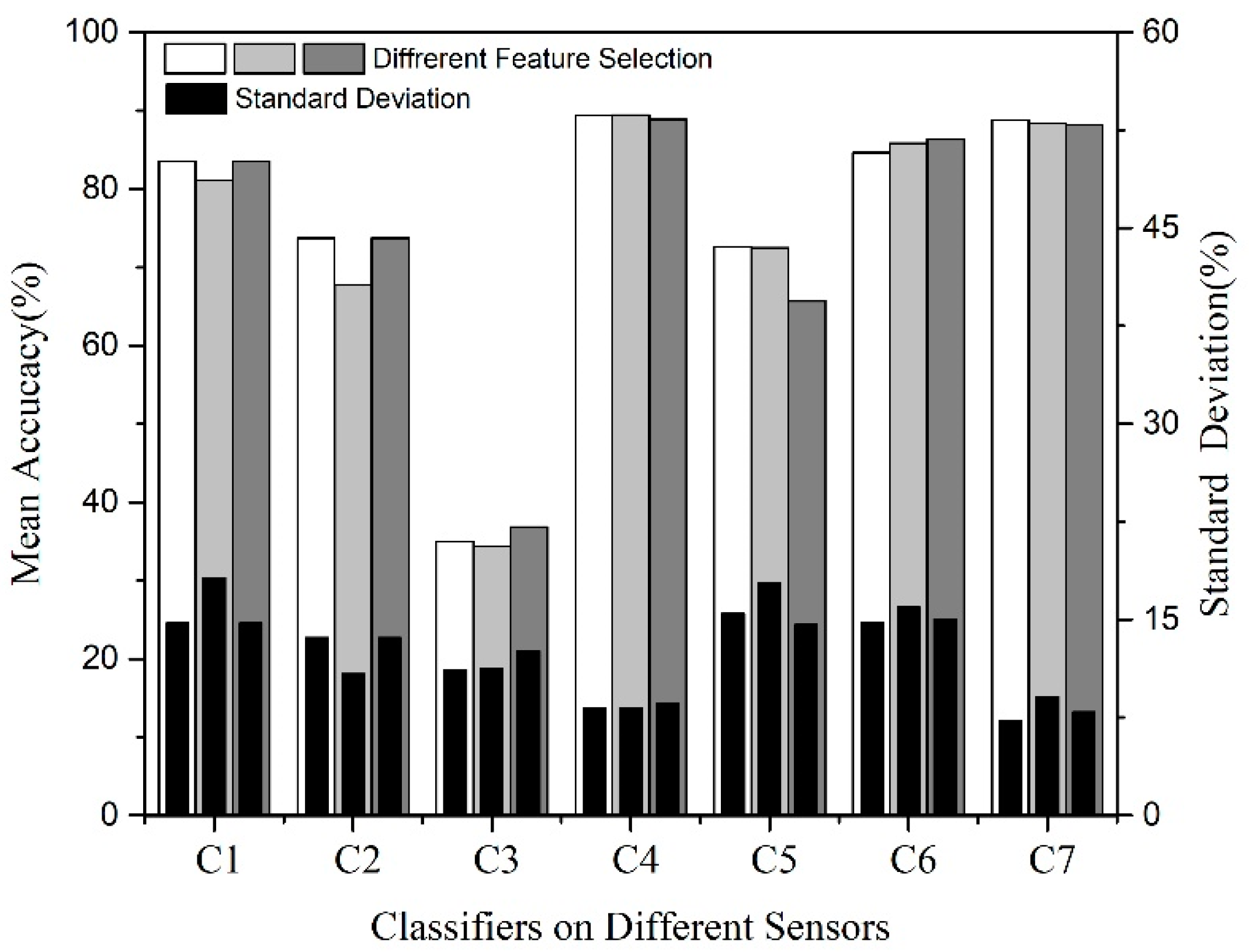
5.1. Separate Classifier Results

Seven classifier clusters based on the seven different sensor datasets, including three single-sensor datasets, three dual-sensor datasets, and one triple-sensor dataset, have been evaluated. Each cluster included three classifiers generated by different random feature selections from the same dataset to enhance the diversity of classifier. The mean and standard deviation of the classification accuracy of the 7 × 3 classifiers are shown in Figure 5. It is seen that within the same classifier cluster, the mean and standard deviation of the classification accuracy are equivalent to each other. Overall, the classifiers yielded better accuracy with more sensor inputs, e.g., the classifiers in the C7 cluster had the best accuracy of activity type classification.

5.2. PA Types Identification of Different Classifier Clusters

So as to combine the different base classifiers through the class-specific weighted majority voting, it is essential to balance the voting weight set of these different classifier combinations. Furthermore, due to the relation of these classifiers to the instances from different datasets, diverse confidences and accuracies on classifying the PA types were yielded. Hence, the average voting weights of these base classifiers were calculated and presented in

Table 3. The voting weights setting of different sensor classifiers for different PA types.

PA Types	The Voting Weights (%)
	C1	C2	C3	C4	C5	C6	C7
CW	75.29	95.29	0	98.82	96.47	82.35	97.65
C1	83.45	82.07	51.03	94.48	91.72	88.97	93.79
T3	58.24	92.94	70.59	93.53	92.35	62.35	92.94
T4	67.23	84.87	9.24	92.44	84.87	68.91	92.44
FP	100.0	16.13	0	98.39	64.52	100.0	98.39
VA	96.77	80.65	0	98.39	69.35	93.55	95.16
BA	76.19	42.86	0	73.81	61.90	76.19	73.81
MB	91.67	45.24	22.62	86.90	54.76	91.67	86.90
TE	80.65	58.06	0	77.42	56.45	82.26	79.03
T6	95.24	97.62	0	95.24	90.48	100.0	100.0

below. It can be seen that the base classifiers have achieved different accuracies (voting weights) on PA label prediction. The different sensor combinations probably reflect the divergences among the different PA types.

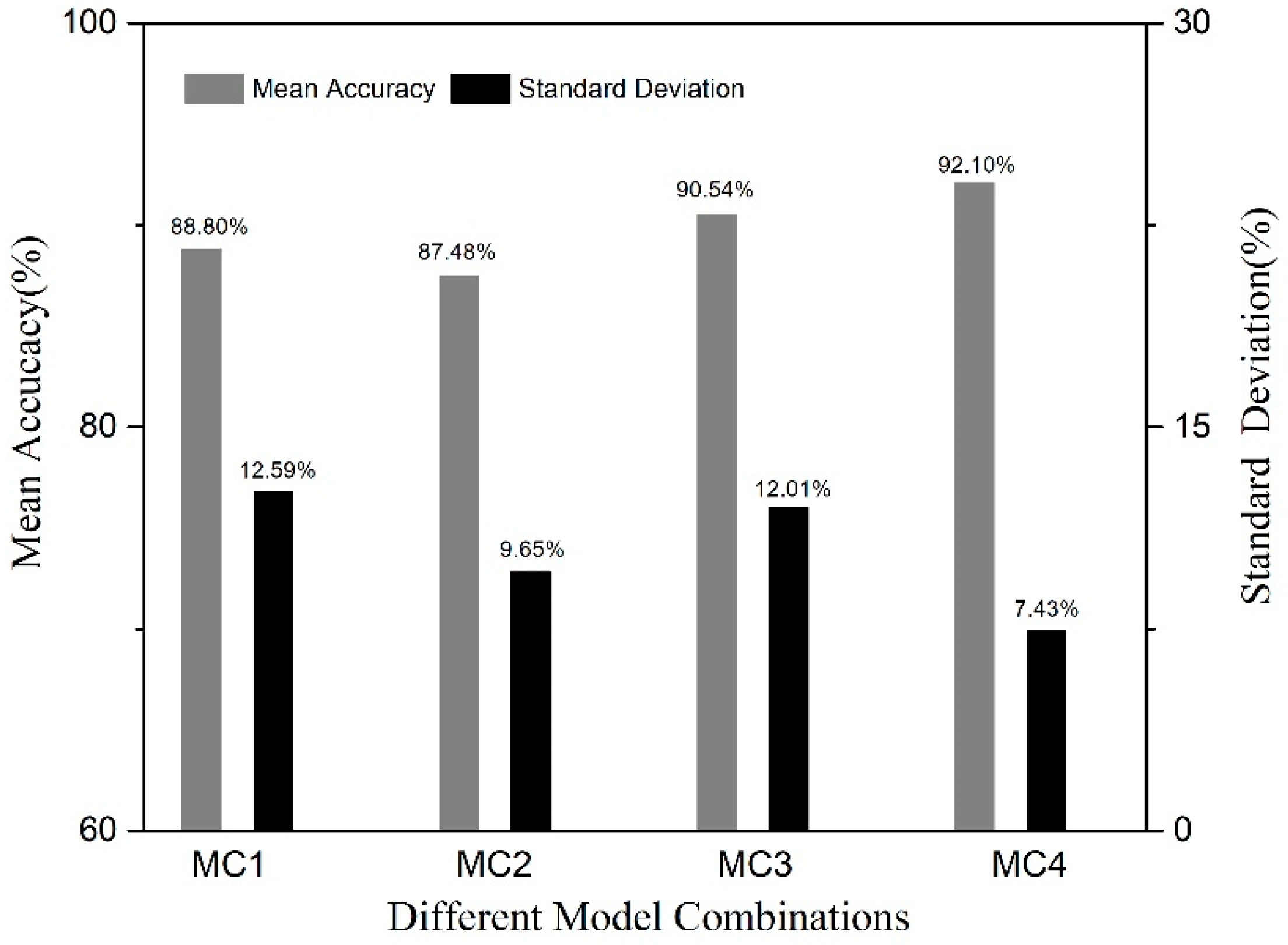
5.3. Results of Different Model Combinations

The capability of this model combination system is in view of the number, type, and identification accuracy of the base classifiers selected. Based on that, a variety of attempts on how to make a combination have been experimented and evaluated. A description of these different model combinations are listed in

Table 4. Definitions of different model combinations.

Model Combination	Definition of Different Combinations
MC1	Classifier of C7.
MC2	A combination of classifiers of C1, C2 and C3.
MC3	A combination of classifiers of C4, C5 and C6.
MC4	A combination of all the classifiers (C1 + C2 + C3 + C4 + C5 + C6 + C7).

, where MC1 assigns the classifiers of C7, MC2 gathers the classifiers of C1, C2, and C3, while MC3 gathers the classifiers of C4, C5, and C6, and MC4 gathers all the classifiers (C1–C7).

For these constructed classifiers, features were randomly selected three times for each sensor dataset, which resulted in three different classifiers in each classifier cluster. Theoretically, the more classifiers that are generated, the better the combination result will be. On the other hand, the more the classifiers, the more computational resources are needed. Thus, a study has been conducted to investigate how the number of different classifiers generated in each classifier cluster affected the classification performance. Figure 6 shows the mean and standard deviation of the classification accuracy of the model combination corresponding to different numbers of feature selection. It is seen that when the feature selection times exceeded three, the performance of the model combination classifier reached a plateau and had little variation.

Figure 7 illustrates the PA classification results of the various model combination classifiers E1–E4. It is seen that the more classifiers and more sensor datasets included in the model combination classifier, the better the result was. For example, the classifier E4 integrated all the classifiers (total 21), and it yielded the best classification mean accuracy of 92.1% with the smallest standard deviation of 7.43%.

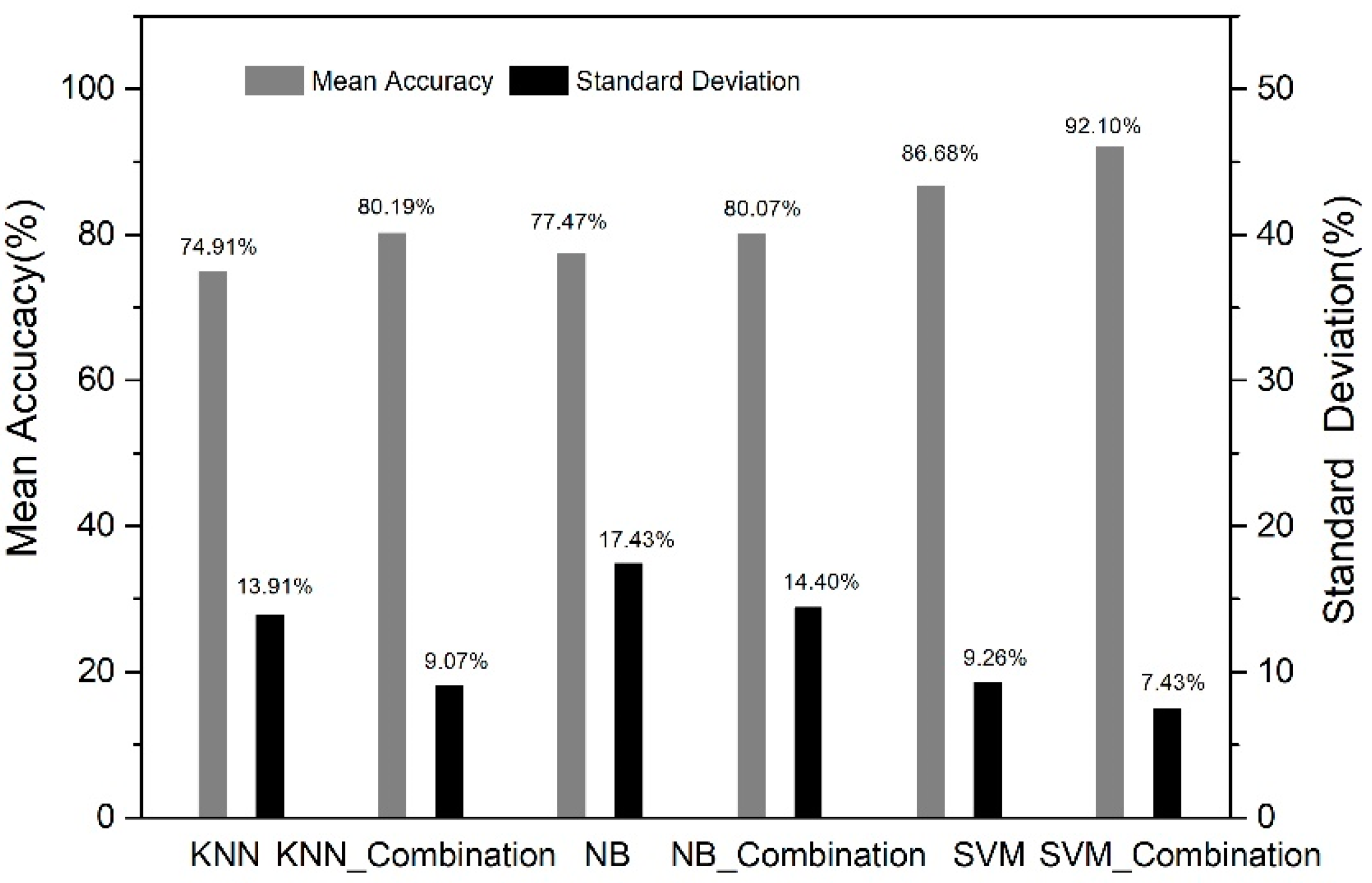
5.4. Comparison between Model Combination and Non-Combination Classifiers

The comparison between the model combination and non-combination classifiers is shown in Figure 8. Three different base classification algorithms, k-nearest neighbor (KNN), naive Bayes (NB) and support vector machine (SVM), were calculated and compared. For all three base classification algorithms, their model combination classifiers had better overall performance than non-combination versions, reflected by the higher mean accuracies and lower standard deviations. Among these model combination classifiers, the SVM based model combination classifier provided the best performance improvement of 6.3% over the non-combination version. Specifically, compared with the non-combination SVM classifier, the model combination classifier improved the mean accuracy from 86.6% to 92.1% and decreased the standard deviation from 9.26% to 7.43%. Confusion matrices of the classification accuracies of the ten different PA types with respect to the combination and non-combination SVM classifiers are shown in

Table 5. Classification Results Comparison.

Predict PA Type		True PA Type
		CW	C1	T3	T4	FP	VA	BA	MB	TE	T6
Model Combination with CWMV	CW	97.56	0	0	0	7.12	0	0	0	0	0
	C1	0	92.91	0.86	0	0	2.38	0	0	0	0
	T3	0	0	75.00	0	0	0	0	0	0	0
	T4	0	0	2.59	94.95	0	0	0	0	0	0
	FP	2.44	5.51	2.59	2.02	92.86	0	0	5.77	0	0
	VA	0	1.57	18.97	0	0	97.62	0	1.92	4.55	0
	BA	0	0	0	3.03	0	0	95.56	11.54	0	1.67
	MB	0	0	0	0	0	0	0	80.77	0	0
	TE	0	0	0	0	0	0	0	0	95.45	0
	T6	0	0	0	0	0	0	4.44	0	0	98.33
SVM	CW	70.21	0.88	0	0	16.67	0	0	0	0	0
	C1	21.28	90.27	1.89	0	1.67	9.09	0	0	0	0
	T3	0	0	78.30	0	0	7.27	0	0	0	0
	T4	0	0	0	90.48	0	1.82	0	2.13	0	0
	FP	8.51	5.31	0.94	0.95	81.67	5.45	0	8.51	0	0
	VA	0	3.54	17.92	0.95	0	76.36	0	2.13	0	0
	BA	0	0	0	7.62	0	0	100.0	0	4.55	3.17
	MB	0	0	0.94	0	0	0	0	87.23	0	0
	TE	0	0	0	0	0	0	0	0	95.45	0
	T6	0	0	0	0	0	0	0	0	0	96.83

. The areas in grey are the specific classification precisions of the model for all the activities. Furthermore, a box chart of the classification result of these two algorithms was given in Figure 9. It shows that the model combination classifier performed better and obtained more stable classification ability than the non-combination one for all the ten PA types.

5.5. Comparison Between Voting Methods

For this multi-sensor model combination system, the comparison between the class-specific weighted majority voting and the normal weighted majority voting is shown in Figure 10. Compared with the normal weighted majority voting, the class-specific weighted majority voting improved the mean accuracy from 90.2% to 92.1% and decreased the standard deviation from 7.70% to 7.43%. Because different sensors and classifiers have different accuracies and voting weights to different PA types, the model combination with class-specific weighted majority voting has better performance than the traditional mean value majority voting combination for the activity monitoring system.

6. Conclusions

In this paper, a combination of models with the CWMV system was designed and evaluated for the multi-sensor activity monitoring system (WIMS). Different sensor and classifier combinations would achieve different performances on recognizing different PA patterns. Based on that, the approach proposed splices the data measured by the three sensor nodes into a new data frame to enhance the diversity of the model inputs and combines the multiple different classifiers according to the classification accuracies of the different PA types. For the non-combination classifier, all the data obtained from the multiple sensors were merged as a single set of features, which assumes that all the data obtained from the various sensors were sampled from one multivariate statistical distribution. On the other hand, the method in this study maintains the statistical distribution of each sensor dataset of its own and fuses their decisions with the class-specific weighted majority voting. Compared to the non-combination classifier, the CWMV system has achieved higher mean accuracies, lower standard deviations, and better generalization capability with “leave-one-subject-out” cross-validation.

Although promising results have been demonstrated in this study, there are limitations that need to be addressed. For example, CWMV has obtained a higher classification accuracy at the expense of taking more computational resources than non-combination classifiers. More participants will need to be involved in future research to improve the robustness in generalizability. Furthermore, there are several issues that remain unanswered, e.g., (1) number and type of sensors to be used to achieve the best classification performance, (2) sensor placement, (3) features and classifiers that are optimal for the model combination system, and (4) comparison of this method with other model combination methods for PA classification. These issues will be addressed in future result to further improve the performance and robustness of the multi-sensor activity monitoring system.

References

1. Caspersen, C.; Powell, K.; Christenson, G. Physical activity, exercise, and physical fitness: Definitions and distinctions for health-related research. Public Health Rep. 1985, 100, 126–131. [Google Scholar] [PubMed]
2. Hendelman, D.; Miller, K.; Bagget, C.; Debold, E.; Freedson, P. Validity of accelerometry for the assessment of moderate intensity physical activity in the field. Med. Sci. Sports Exerc. 2000, 32, 442–449. [Google Scholar] [CrossRef]
3. Scanaill, C.; Carew, S.; Barralon, P.; Noury, N.; Lyons, D.; Lyons, G. A review of approaches to mobility telemonitoring of the elderly in their living environment. Ann. Biomed. Eng. 2006, 34, 547–563. [Google Scholar] [CrossRef] [PubMed]
4. Staudenmayer, J.; Pober, D.; Crouter, S.; Bassett, D.; Freedson, P. An artificial neural network to estimate physical activity energy expenditure and identify physical activity type from an accelerometer. J. Appl. Physiol. 2009, 107, 1300–1307. [Google Scholar] [CrossRef] [PubMed]
5. Cao, J.; Li, W.; Ma, C.; Muhammad, S.; Stephan, B.; Ozlem, I.; Hans, S.; Paul, H. Complex human activity recognition using smartphone and wrist-worn motion sensors. Sensors 2016, 16, 426. [Google Scholar]
6. Ermes, M.; Parkka, J.; Mantyjarvi, J.; Korhonen, I. Detection of daily activities and sports with wearable sensors in controlled and uncontrolled conditions. IEEE Trans. Inf. Technol. Biomed. 2008, 12, 20–26. [Google Scholar] [CrossRef] [PubMed]
7. Feng, Z.; Mo, L.; Li, M. A Random Forest-based ensemble method for activity recognition. In Proceedings of the 2015 37th Annual International Conference of the IEEE Engineering in Medicine and Biology Society (EMBC), Milan, Italy, 25–29 August 2015. [Google Scholar]
8. Altini, M.; Penders, J.; Vullers, R.; Amft, O. Estimating energy expenditure using body-worn accelerometers: A comparison of methods, sensors number and positioning. Biomed. Health Inform. 2014, 19, 219–226. [Google Scholar] [CrossRef] [PubMed]
9. Liu, S.; Gao, R.; Freedson, P. Design of a wearable multi-sensor system for physical activity assessment. In Proceedings of the 2010 IEEE/ASME International Conference on Advanced Intelligent Mechatronics 2010, Montreal, ON, Canada, 6–9 July 2010; pp. 254–259. [Google Scholar]
10. Carbonell, J.G. Machine learning research. ACM Sigart Bull. 1981, 18, 29. [Google Scholar] [CrossRef]
11. Pober, D.; Staudenmayer, J.; Raphael, C.; Freedson, P. Development of novel techniques to classify physical activity mode using accelerometers. Med. Sci. Sports Exerc. 2006, 38, 1626–1634. [Google Scholar] [CrossRef] [PubMed]
12. Yudistira, N.; Kurita, T. Gated spatio and temporal convolutional neural network for activity recognition: Towards gated multimodal deep learning. EURASIP J. Image Video Process. 2017, 2017, 85. [Google Scholar] [CrossRef]
13. Naik, G.; Kumar, K. Twin SVM for gesture classification using the surface electromyogram. IEEE Trans. Inf. Technol. Biomed. 2010, 14, 301–308. [Google Scholar] [CrossRef] [PubMed]
14. Shao, S.; Shen, K.; Ong, C.; Wilder-Smith, E.; Li, X. Automatic EEG artifact removal: A weighted support vector machine approach with error correction. IEEE Trans. Biomed. Eng. 2009, 56, 336–344. [Google Scholar] [CrossRef] [PubMed]
15. Umakanthan, S.; Denman, S.; Fookes, C. Activity recognition using binary tree SVM. In Proceedings of the IEEE Workshop on Statistical Signal Processing Proceeding, Gold Coast, VIC, Australia, 29 June–2 July 2014; pp. 248–251. [Google Scholar]
16. Liu, S.; Gao, R.; John, D.; Staudenmayer, J.; Freedson, P. Multi-sensor data fusion for physical activity assessment. IEEE Trans. Biomed. Eng. 2012, 59, 687–696. [Google Scholar] [PubMed]
17. Yuan, Y.; Wang, C.; Zhang, J. An Ensemble Approach for Activity Recognition with Accelerometer in Mobile-Phone. In Proceedings of the IEEE International Conference on Computational Science and Engineering IEEE Computer Society, Chengdu, China, 19–21 December 2014; pp. 1469–1474. [Google Scholar]
18. Kuncheva, L.; Whitaker, C. Measures of diversity in classifier ensembles and their relationship with the ensemble accuracy. Mach. Learn. 2003, 51, 181–207. [Google Scholar] [CrossRef]
19. Zheng, Y.; Wong, W.K.; Guan, X.; Trost, S.G. Physical activity recognition from accelerometer data using a multi-scale ensemble method. In Proceedings of the Twenty-Seventh AAAI Conference on Artificial Intelligence, Bellevue, WA, USA, 14–18 July 2013; AAAI Press: Menlo Park, CA, USA, 2013. [Google Scholar]
20. Ravi, N.; Dandekar, N.; Mysore, P.; Littman, M. Activity recognition from accelerometer data. In Proceedings of the Seventeenth Conference on Innovative Applications of Artificial Intelligence, Pittsburgh, PA, USA, 9–13 July 2005; pp. 1541–1546. [Google Scholar]
21. Kaur, A.; Sharma, S. Human Activity Recognition Using Ensemble Modelling. In International Conference on Smart Trends for Information Technology & Computer Communications; Springer: Singapore, 2016. [Google Scholar]
22. Mo, L.; Liu, S.; Gao, R.; Freedson, P.S. Multi-Sensor Ensemble Classifier for Activity Recognition. J. Softw. Eng. Appl. 2012, 5, 113–116. [Google Scholar] [CrossRef] [Green Version]
23. Yoon, J.; Zame, W.R.; van der Schaar, M. ToPs: Ensemble learning with trees of predictors. IEEE Trans. Signal Process. 2018, 66, 2141–2152. [Google Scholar] [CrossRef]
24. Opitz, D.; Maclin, R. Popular ensemble methods: An empirical study. J. Artif. Intell. Res. 1999, 11, 169–198. [Google Scholar] [CrossRef]
25. Dos Santos, E.M.; Sabourin, R.; Maupin, P. Overfitting cautious selection of classifier ensembles with genetic algorithms. Inf. Fusion 2009, 10, 150–162. [Google Scholar] [CrossRef]
26. Breiman, L. Bagging predictors. Mach. Learn. 1996, 24, 123–140. [Google Scholar] [CrossRef] [Green Version]
27. Shawkat, A.B.M.; Dobele, T. A novel classifier selection approach for adaptive algorithms. In Proceedings of the IEEE/ACIS International Workshop on e-Activity, Melbourne, QLD, Australia, 11–13 July 2007; pp. 532–536. [Google Scholar]
28. Freund, Y.; Schapire, R. A decision-theoretic generalization of on-line learning and an application to boosting. In Lecture Notes in Computer Science; Springer: Berlin/Heidelberg, Germany, 1995; pp. 23–37. [Google Scholar]
29. Gashler, M.; Giraud-Carrier, C.; Martinez, T. Decision tree ensemble: Small heterogeneous is better than large homogeneous. In Proceedings of the IEEE Seventh International Conference on Machine Learning and Application, San Diego, CA, USA, 11–13 December 2008; pp. 900–905. [Google Scholar]
30. Kuncheva, L. Combining Pattern Classifiers: Methods and Algorithms; Wiley-Interscience: Hoboken, NJ, USA, 2004. [Google Scholar]
31. Remya, K.R.; Ramya, J.S. Using weighted majority voting classifier combination for relation classification in biomedical texts. In Proceedings of the 2014 International Conference on Control, Instrumentation, Communication and Computational Technologies (ICCICCT), Kanyakumari, India, 10–11 July 2014. [Google Scholar]
32. Markov, Z.; Russell, I. Introduction to data mining. In An Introduction to the WEKA Data Mining System; China Machine Press: Beijing, China, 2006. [Google Scholar]
33. Mo, L.; Liu, S.; Gao, R.; John, D.; Staudenmayer, J.; Freeson, P.S. Wireless Design of a Multi-Sensor System for Physical Activity Monitoring. IEEE Trans. Biomed. Eng. 2012, 59, 3230–3237. [Google Scholar]
34. Gao, L.; Bourke, A.K.; Nelson, J. Evaluation of Accelerometer Based Multi-Sensor versus Single Activity Recognition System. Available online: http://dx.doi.org/10.1016/j.medengphy.2014.02.012 (accessed on 11 March 2014).
35. Gravina, R.; Alinia, P.; Ghasemzadeh, H. Multi-Sensor Fusion in Body Sensor Networks: State-of-the-Art and Research Challenges. Available online: http://dx.doi.org/10.1016/j.inffus.2016.09.005 (accessed on 13 September 2016).
36. Chang, C.; Lin, C. LIBSVM: A library for support vector machines. ACM Trans. Intell. Syst. Technol. 2011, 2, 27. [Google Scholar] [CrossRef]
37. Lapin, M.; Hein, M.; Schiele, B. Learning Using Privileged Information: SVM+ and Weighted SVM. Available online: http://dx.doi.org/10.1016/j.neunet.2014.02.002 (accessed on 14 February 2014).
Figure 1. Multi-sensor model combination system architecture block diagram.
Information 10 00197 g001
Figure 2. The overall architecture of the multi-sensor activity monitoring system.
Information 10 00197 g002
Figure 3. The setup of the WIMS.
Information 10 00197 g003
Figure 4. Features extraction and selection.
Information 10 00197 g004
Figure 5. Classification results with different sensor datasets and feature selections.
Information 10 00197 g005
Figure 6. Classification results with respect to different feature selection times.
Information 10 00197 g006
Figure 7. Classification results among different model combinations.
Information 10 00197 g007
Figure 8. Performance comparison between the model combination and non-combination classifiers.
Information 10 00197 g008
Figure 9. Statistical distributions of classification results of the model combination and non-combination SVM classifiers.
Information 10 00197 g009
Figure 10. Performance comparison between the class-specific weighted majority voting and the traditional weighted majority voting.
Information 10 00197 g010