Abstract
The information contained within Call Details records (CDRs) of mobile networks can be used to study the operational efficacy of cellular networks and behavioural pattern of mobile subscribers. In this study, we extract actionable insights from the CDR data and show that there exists a strong spatiotemporal predictability in real network traffic patterns. This knowledge can be leveraged by the mobile operators for effective network planning such as resource management and optimization. Motivated by this, we perform the spatiotemporal analysis of CDR data publicly available from Telecom Italia. Thus, on the basis of spatiotemporal insights, we propose a framework for mobile traffic classification. Experimental results show that the proposed model based on machine learning technique is able to accurately model and classify the network traffic patterns. Furthermore, we demonstrate the application of such insights for resource optimisation.
1. Introduction
With the mammoth development in mobile and the internet of things (IoT) technologies, it can be anticipated that in next generation-networks (NGN) everything will be connected. The number of mobile devices such as smart phones, tablets, and wearable devices are on the rise exponentially. So, the next generation-networks will be considered as worldwide wireless networks (WWWN). According to a report provided by Ericsson, in future there will be billions of connected devices [1]. Such a huge connectivity of wireless devices will increase the data traffic volume largely. During the last decade, 4000 fold increase occurred in the data volume and it will increase further in next-generation networks (NGN) [2]. According to CISCO report, wireless traffic is generating 24 Exabyte (EB) data per month and it is continuously growing [3].
Mobile network traces provide extensive information about the network and its subscribers’ behavior. However, the analysis and modeling of network traces is a non-trivial task [4]. The existing solutions for understanding and modeling of network traces and its pattern provide limited information. As the key factors affecting the network traffic variations are still needed further research. Such limitations, increase the operation cost of the cellular network and degrade the quality of service especially in densely populated areas.
The useful insights obtained from the network traffic analysis are highly valuable for network operators as well as network subscribers mainly in the case of ultra-dense networks [5,6]. If the cellular network traffic patterns are accurately predicted and modeled, then the network operators can sub-divide the network coverage area into different sub-regions according to the predicted traffic pattern. Hence, network resources can be distributed to sub-regions according to their traffic conditions. Such traffic modeling would be beneficial for mobile users in terms of better quality of service. In addition, the network traffic optimization would also be helpful for network operators in making efficient operational schemes [7].
Motivated from the above work, in this article, we classify and monitor the network traces of a real cellular network by applying a clustering based artificial neural network model. The network traces analyzed in this work are call details record (CDR). The CDR data contains both spatial and temporal information. On the basis of the spatiotemporal feature of CDR data, we performed spatial and temporal analysis separately and extracted useful insights about the subscribers as well as the network. These insights will be helpful in meeting QoS requirements of NGN and improving throughput. The main contributions of this work are as under:
- We analyze the CDR data of large scale cellular network. The dataset contains the CDR activity for Milan city. Such a vast dataset helps us to understand and model the network traffic for urban, suburban and rural areas.
- We perform the spatiotemporal analysis of CDR data. For a spatiotemporal analysis of CDR data, we also investigate the spatial and temporal correlation for understanding and extracting mobile traffic patterns.
- We utilize machine learning’s unsupervised clustering algorithm for categorizing the mobile traffic patterns in different groups/classes. Then using the clustering results, we train a neural network for classification of network traffic.
- Lastly, we present a generic data-driven resource allocation approach for cellular networks. The approach utilizes unsupervised clustering and a trained neural network to classify cells in a cluster according to the respective activity level.
The rest of the paper is organized as follows: In Section 2, we present the related work. Section 3 presents the system model and description of the dataset. Section 4 introduces the reader to the underlying dynamic nature and spatio-temporal characteristics of the CDR data at hand, which then forms the basis for network activity classification and prediction using these spatio-temporal characteristics. In Section 5, we describe the proposed clustering based classification model. A generic data-driven resource allocation/management approach for cellular network is presented in Section 6. Finally, we conclude our work in Section 7.
2. Related Work
Understanding of network traces produces numerous benefits for social network analysis [8,9] as well as for cellular network analysis [10,11]. The network traces are divided into two categories (i) traces obtained from the mobile devices (ii) traces obtained from the mobile operators. In the first category, network information such as network performance, geographic information, service quality, throughput, and latency are monitored automatically by the applications (APPs) running on the mobile devices [12,13]. The limitation of this approach is that the network information/traces are obtained only for a limited number of users who have the app installed on their devices. So the insights obtained from such network traces are not applicable for monitoring the large-scale mobile network. On the other hand, the traces obtained from network operator provide a bundle of information such as users mobility, service quality, network performance etc for an entire cellular network [14,15]. The insights obtained from these traces are very useful for monitoring the network as well as the behavior of the users [16,17]. The dataset utilized in our work is for a densely populated area, and obtained from the network operator.
During the last decade, the cellular network traces have been mainly analyzed for monitoring human mobility pattern. Deville et al. [18] performed the spatiotemporal analysis of call details record data for estimating the population density. Ficek et al. [19] performed a spatiotemporal analysis of CDRs for understanding user mobility. Some other works for understanding the individuals and collective mobility are presented in [20,21,22,23].
From last few years, the network traces are largely exploited for understanding and modeling the network dynamics. Lee et al. [24] described that Log normal distribution efficiently approximated the network traffic density. Wang et al. [25] also performed the spatiotemporal analysis of cellular traces and showed that the cellular traces follow trimodal distribution. In addition, Kashif et al. [26] analyzed network traces for anomaly detection and traffic prediction for cellular networks.
Unlike the existing work, in this article, we focus on a spatiotemporal analysis of CDRs for optimizing and categorizing network traffic. The categorization of network traces will be helpful in efficiently monitoring and optimizing network traffic.
3. System Model and Dataset Description
In this section, we discuss the framework of the proposed system model and describe the description of the observed dataset. In proposed architecture, the area of the city (Milan) is divided into four subregions namely, high activity area, medium activity area, low activity area and very low activity area. This division is based on the CDR activity level of the mobile phone’s subscribers. The high activity area mainly consists of the city center where many shopping malls, buildings, hospitals, and other busy centers are located. The areas in the surroundings of the city center are considered to be located in the medium activity area. Similarly, the areas far away from the city center are low activity and very low activity areas. Figure 1 represents the overall framework.
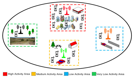
Figure 1.
Overall architecture.
The overall system model presented in our work comprises of three stages: (i) data preparation and analysis step, (ii) clustering analysis step and (iii) CDRs classification step. Figure 2 represents the layered structure of the proposed model.
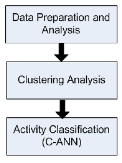
Figure 2.
Major Steps.
In the proposed model, firstly CDR data is collected and stored. The available data is spatiotemporal, so spatial and temporal analysis are performed for observing the spatial and temporal dependencies. Then, from clustering analysis, the CDR activities are categorized into different groups according to spatiotemporal variation and the entire region is divided into four different sub-regions. After the clustering analysis, an artificial neural network (ANN) is trained based on the clustering results for classification of future network traffic (CDRs). The clustering analysis is performed prior to the training of ANN for transforming the problem from unsupervised to a supervised multi-class classification problem. The proposed model is named as clustering based ANN (C-ANN) model. The overall system model is represented in Figure 3.
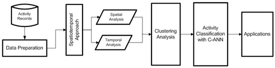
Figure 3.
System model.
3.1. Description of Dataset
The dataset used for analysis is for Telecom Italia for the city of Milano and is made public in 2014 after the contest of Big data challenge [27]. This is spatiotemporal data because it contains both spatial and temporal aspects of subscribers and networks. Temporally, two months data is divided into days where each day data is further aggregated on 10 min interval. On the other hand, spatially data is divided into grids. The whole city of Milan is divided into 100 × 100 grids whereas each grid has an area of 0.05 square kilometers [27]. Figure 4 represents the layout of spatial grids distributed over the city of Milan, Italy.
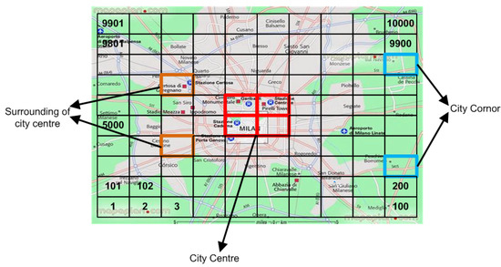
Figure 4.
100 × 100 grids distribution over Milan.
Table 1 represents samples of this dataset. The dataset consists of the following fields. (i) Cell ID, which represents the location of cells(grids), (ii) Timestamp, shows the time of the CDR activity, (iii) Received/Sent SMS, it represents the number of SMS received and sent at each time step, and (IV) Incoming/outgoing calls, shows the number of incoming and outgoing calls.

Table 1.
Telecom Italia dataset fields.
3.2. Data Preparation
The obtained dataset was in raw form, so the dataset has the different type of impurities and irregularities. Such irregularities include missing values, unrecognized numbers, and misleading patterns. So data must be prepared before performing the analytical step. Data preparation is helpful in improving output quality and reducing processing overhead.
As the dataset is temporarily aggregated on 10 min time interval, but in dataset values at some timestamps are missing. As the CDR activity is happening before and after missing value’s time interval. So it is obvious that the CDR activity will be also happening at missing value’s time interval. So for handling missing values in the dataset, missing values are replaced with the average values of the previous and next timestamp values. The expression for finding the missing CDRs is shown in Equation (1)
With the help of expression presented in Equation (1), the proposed framework can work for partially available information. For example, wherever required, we have taken an average of previous and next value to get the current missing value.
4. Spatio-Temporal Approach
As after the data preprocessing, we summarize data in three columns. The first column has information about grid ID (Grid ID represents the location of the activity in Milan city). The second column contains the time of the particular activity and third activity level (we sum up the values of received SMS, sent SMS out, incoming calls and outgoing calls and named it as activity level). We may better understand dynamic nature of CDR data by analyzing it in both spatial and temporal context. This static analysis signifies the relationship of CDR activity in both spatial and time domains. Based on the spatio-temporal charecteristics, we develop a framework for mobile traffic classification.
4.1. Spatial Approach
In the spatial approach, we have fixed the temporal variation. CDRs activities at a specific time period are observed over the entire city of Milan. For this purpose, the data of a specific day is taken. After data preparation step, the data is further aggregated on the three-hour interval. Hence, we have data at eight different time slots for an overall period of 24 h. In this way, CDR activity of the entire Milan city is observed for a day.
The variation in CDR activities for a whole city of Milan at a specific time interval (12 pm to 3 pm) is shown in Figure 5. For ease of visualization, the Milan city divided into 100 × 100 grids is downsample to 5 × 5 grid size. Figure 5 shows spatial variation of CDR activities with both 100 × 100 and 5 × 5 grid size. We can clearly detect the variation in CDR activities from 5 × 5 grid size in Figure 5. It is obvious that the CDR activities are high at the center of the city and as we move away from the center the CDR activity reduces. Similarly, the variation in CDR activities for a whole day is represented in Figure 6 with grid size of 5 × 5. It is clear from Figure 6 that the variation in CDR activities follows the same pattern for the whole day.
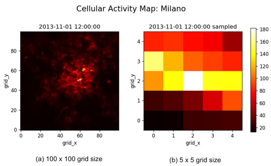
Figure 5.
Spatial variaton of CDR activity over Milan at a specific time instant.
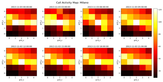
Figure 6.
Spatial Variation of CDR activities over the City of Milan for one day’s Time intervals.
Spatial Correlation
It is observed that the CDRs activities are not distributed uniformly over the city of Milan because of different dynamics of Milan sub-regions such as commercial, residential, rural etc. A popular and widely adapted parameter, Pearson correlation coefficient r is used for measuring the variation in spatial correlation [28]. The variation in spatial correlation among the targeted grids, for example, the grids in the center of the city, and grids in the surrounding of the targeted grids is calculated with Pearson correlation coefficient. Equation (2) represents the mathematical expression of Pearson correlation coefficient.
where is the standard deviation, cov represents the covariance, is the target grid and represents the grid in the vicinity of the target grid. Figure 7 represents the variation in spatial correlation for the entire city of Milan. As we already downsampled the 100 × 100 grids of Milan into grid size of 5 × 5. So in 5 × 5 grid size, one cell represents 400 grids. In Figure 7, the centre cell (3,3) represents grids number 4801 to 5200 and the first cell (1,1) in Figure 7 shows the grids from 1 to 400. Hence, the center cell (3,3) is considered as the target cell for Pearson correlation calculation. It is observed that the spatial correlation is high between the targeted cell and the cells near to target cell and spatial correlation is low between the target cell and the cells far away from the target cells. Hence, the spatial correlation is dependent on the distances between cells. On the other hand, another interesting fact is observed from Figure 7, as the cell (2,3) and (4,3) are at the same distance from the target cell (3,3) but spatial correlation differs a lot. This phenomenon shows that spatial correlation is also location dependent.
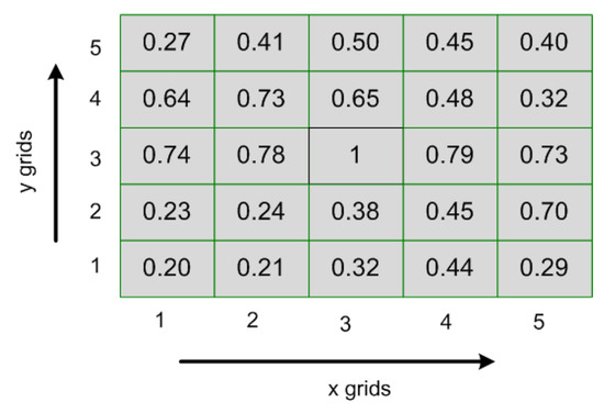
Figure 7.
Spatial correlation.
Hence, from the spatial analysis of CDR activities, the spatial feature can be extracted. The CDR activities of entire Milan region are divided into different domains such as CDR activities from a high-interest area, medium interest area, and low-interest area.
4.2. Temporal Approach
In the temporal approach, we have fixed the spatial variation and observed the CDR activities for a day, a week and a month. To fix the spatial variation, we observed CDR activities for a specific grid. The simulations results for temporal analysis show that CDR activities are very high in the evening and very low at midnight. The time-series curves for CDR activity are shown in Figure 8 and Figure 9. In Figure 8 the temporal variation of CDR activities aggregated on ten minutes interval over a period of one day is shown, whereas the varaition in CDR activities aggregated on one hour interval over a period of one week is shown in Figure 9. We have sum up the values of incoming calls and outgoing calls to quantify the activity level, as represented in Equation (3):
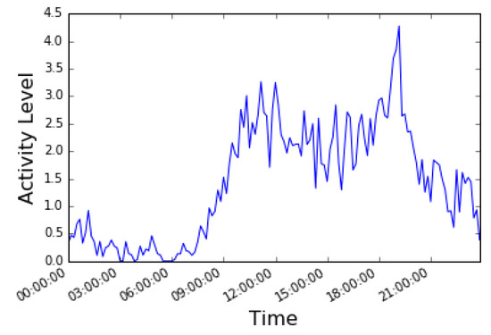
Figure 8.
Variation of CDR activity over Milan for 24 hours.
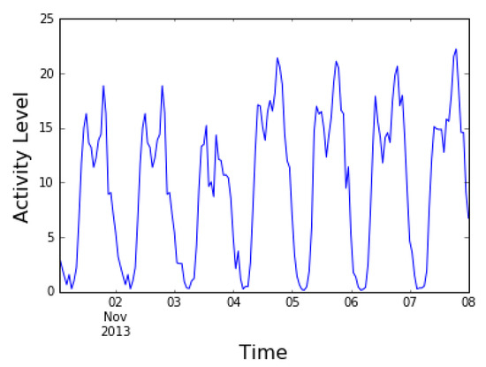
Figure 9.
Variation of CDR activity over a week period.
It is shown in Figure 8 that CDR activity is increasing from midnight to morning, then decreasing from noon to afternoon and increasing from evening to mid-night. Similar pattern of CDR activities are observed for a day, a week and a month. The CDR activity over a week period is represented in Figure 9.
Temporal Correlation
Temporal correlation is observed for measuring the temporal dependencies in the CDRs. Autocorrelation function (ACF) is widely used for measuring temporal variation of time series data [29]. For observing the temporal dependencies in time series, ACF calculates the correlation of time series with the previous observations of the same time series called lags (this is also termed as serial correlation). Equation (4) shows the mathematical representation of temporal correlation.
where T is the total number of time steps in the time series and is the average value of time series data. Figure 10 represents the autocorrelation function for 168 lags. 168 lags represent the temporal dependencies of CDRs for a week period with a step size of one hour. From Figure 10, it is observed that there is exist an hourly pattern in CDRs because autocorrelation function plot have peaks after every 24 lags.
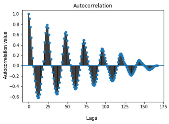
Figure 10.
Temporal correlation over a week period.
So, from the temporal analysis, the temporal feature of CDR activities can be extracted. Temporally, CDR activities can be divided into different domains such as CDR activities during off-peak hours, on-peak hours and normal peak hours.
5. Clustering Driven ANN Model (C-ANN)
After the spatiotemporal analysis of preprocessed data, the later step is to classify CDRs according to their activity levels and spatiotemporal characteristics. For CDR activity classification, firstly, clustering analysis is applied for observing the density of clusters. After that artificial neural network is trained based on the clustering results. The overall classification framework is shown in the Figure 11.
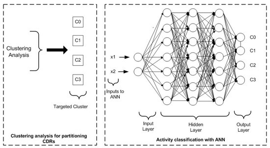
Figure 11.
Activity classification with a clustering driven ANN model.
5.1. Clustering Analysis
5.1.1. Gaussian Mixture Models (GMM) Clustering
Machine learning’s clustering algorithm is adopted for grouping the CDR activities according to their activity level and spatiotemporal characteristics. To identify patterns of variations in CDR activities over the whole city of Milan, CDR activities of entire region are passed through clustering scheme. We applied GMM based clustering scheme on our dataset. One motivation for using GMM is the use of a probabilistic approach for cluster assignment in GMM, which is otherwise not found in k-means clustering and thus, k-means fails to perform well in certain scenarios. In GMM, the cluster is formed on the basis of the probability of each point belonging to an associated cluster. GMM is loosely considered as an extension of k-means with enhanced accuracy. The GMM clustering algorithm is summarized in Algorithm 1.
| Algorithm 1: GMM algorithm |
 |
GMM based clustering analysis on activity data results in four different clusters categorized in different activity-types, as very high activity, high activity, medium activity, and very low activity cluster. Figure 12 represents the GMM based clustering approach at a specific time instant, different clusters are shown with different colors. From Figure 12, it is observed that the cluster form in the center of the region, consists of very high CDR activities. So we named it as very high activity cluster. Similarly, the cluster form near the center of the region also consists of high CDR activities but lower than the central cluster activities. On the other hand clusters further away from central region consists of low CDR activities. Hence, based on the results of clustering analysis, the entire is divided into different sub-regions/groups. For understanding the spatiotemporal as well as the dynamic nature of the source (mobile users), the clustering results at different time instants of a day are shown in Figure 13.
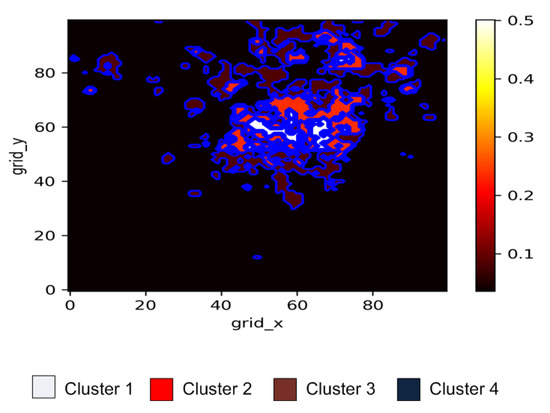
Figure 12.
GMM Clustering.
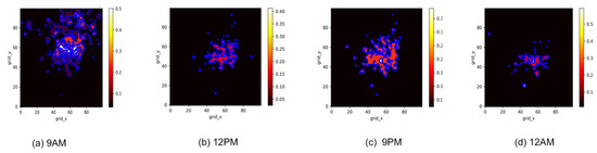
Figure 13.
GMM Clustering at different time instants of a day.
5.1.2. The Criterion for Number of Clusters
Typically, a higher number of clusters leads to over-fitting in the model. To avoid the over-fitting in the clustering model some analytical approaches such as Bayesian information criterion (BIC) and Akaike information criterion (AIC) are adapted. We have plotted BIC and AIC for GMM model. The minimum values of BIC and AIC determine the optimum number of clusters for the model. The BIC and AIC curves for our dataset are shown in Figure 14. From Figure 14, it is observed that using three or four clusters (k = 3, 4) provides an optimal choice for our data.
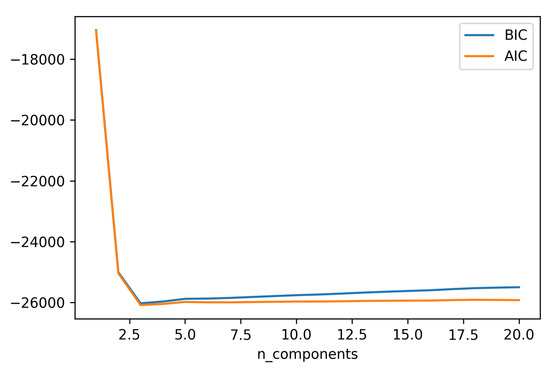
Figure 14.
AIC/BIC for curves for number of clusters.
5.2. C-ANN—Traffic Classification
The proposed clustering based artificial neural network model (C-ANN) is applied for observing the future CDR activity class. With C-ANN, the CDRs activity classification is converted from unsupervised to supervised multi-class classification problem. From the categorical distribution of CDR activities obtained from clustering analysis, targets for C-ANN model are set. C-ANN model classifies CDR activities according to activity levels and spatiotemporal characteristics. The inputs of the C-ANN model are CDR activity level and spatial feature. A spatial feature is obtained from the spatial analysis described in the prior section. The outputs of C-ANN model are multiple classes named C0, C1, C2, and C3 (where C0 represents very high activity cluster/class, similarly C1, C2, C3 represents the cluster/class with medium, low and very low activity).
The CDRs of five days is used for training and testing of C-ANN model. Previously, data (CDRs) is temporally aggregated on one hour time interval, for ease of processing and reducing data overhead. CDR data is also temporally aggregated for three hours time interval for the whole city of Milan. For training of C-ANN, we have used the CDR data temporally aggregated on three hours interval. In this way, there are total eight-time slots for one day. As Milan city is spatially divided into 10,000 grids, so there are 80,000 samples for one day and for five days activities, there is a total of 0.4 million samples. From these samples, 80% samples are used for training and 20% samples for testing of the C-ANN model. Though, it is the simplest approach but outperforms for CDRs activity classification.
Performance Evaluation
In our C-ANN model for activity classification, loss and accuracy are adopted as performance metrics. As in the proposed model, our aim is multi-class classification, so categorical cross entropy is used as a loss function. Simulation results show that training losses and testing losses are decreasing as the number of epochs is increasing. It is shown in Figure 15 that the training loss is decreasing rapidly in the first three epochs and after that reach to a stable state. The testing loss also follows the training loss. This phenomenon shows that the model is fast converging and time efficient. Similarly, training and testing accuracies are increasing as the number of epochs is increasing and reach a stable state after some epochs. Figure 15 and Figure 16 represent training and testing losses and accuracies curves for C-ANN model of activity classification.
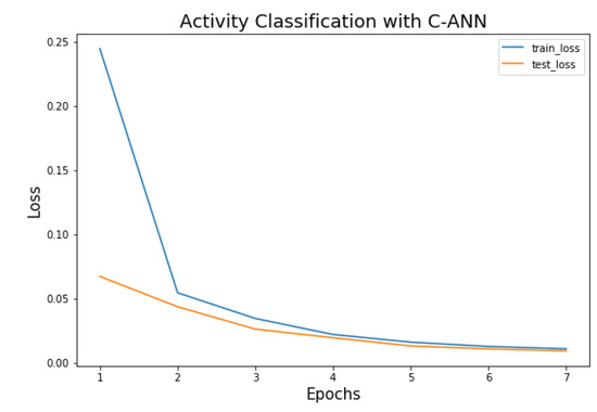
Figure 15.
Training and testing losses of C-ANN Model.
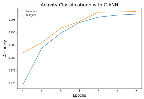
Figure 16.
Training and testing accuracy of C-ANN Model.
Further, C-ANN based classification model can be used in many real-world network scenarios such as spectrum distribution or small cells deployment. For example, the proposed model can be used to identify low and high activity regions. Thus, additional small cells and spectrum can then be allocated to the high activity region. In this way, QoS would be improved and energy consumption would be reduced. For such case, the accuracy of the model is very important, if the proposed model is not able to identify the region accurately then the quality of service will greatly be affected. In next-generation networks, there will be ultra densification of small cells and billions of mobile devices/user equipment, so such type of model is heavily needed for efficient deployment of small cells and improvement in QoS.
6. Insights into CDRs Driven Traffic Optimization Approach
It is observed, from the spatiotemporal analysis performed in Section 4, that network traces have time-varying as well as space varying characteristics. These spatiotemporal characteristics are beneficial for deploying as well as optimizing the cellular network.
In conventional scenarios, resources deployment were not optimized due to lack of advancements in data analytics tool. With the useful insights obtained from the spatiotemporal analysis of network traces, cellular network operators are able to make intelligent decisions which aid in network optimization. The extracted information is also helpful in understanding and predicting future trends of the network traces [30].
The knowledge extracted from spatiotemporal analysis help in predicting the resource requirements at different geographical locations at a specific time perioid. In addition, the mobility pattern of the user is also predcited. For example, in events with big gatherings (say, a soccer world cup match), huge crowd is typically attracted to the venue, which results in network congestion at the particular location for a specific period of time. Hence, with this predicted insights obtained from spatiotemporal analytics, network operators deploy extra resources at the region of interest, which help in avoiding network congestion.
It is a well understood phenomena that resource allocation (such as energy, bandwidth) can be optimized if it is made adaptive based on the specific needs in a geographic location or at a specific time. Similar tasks on optimization can be found in other works where the data analytics is the key behind the optimization. For example, in [31], the authors adopt big data analysis methods to divide densely deployed base stations into groups. Then, each group of base stations are managed with networking mechanisms independently. In this way, the complexity of the networking mechanisms is reduced. Similarly, in [32], it is well described that machine learning based analysis sets a wonderful platform for capacity optimization and topology management in networks. Further motivation can be drawn on the dynamic bandwidth allocation scheme as presented in [33]. In particular, the authors in [33] identify that the user and network related information carried in the network data, were seldom employed to improve a network’s performance. Similarly, the importance of useful insights obtained from data analysis is elaborated for different scenarios in studies undertaken in [34,35].
As we have also observed from the temporal analysis of network traces, that the user follows a specific temporal pattern for a day and week. So the resources can be distributed according to peak hours and off-peak hours. In this way, a large number of network resources can be saved from wasting otherwise, due to low activity.
From the useful insights of spatiotemporal analysis of network traces (CDRs) and traffic classification framework, we have proposed an approach for optimizing network resources. In the proposed approach, cluster set G is divided into k clusters, each cluster is then allocated network resources according to CDR activity level. When cells in the cluster set are assigned to different clusters (according to the respective CDR activity level), a new grid set of optimized cells will arise. As in our proposed approach optimize a network grid after every h hours (3 h in our case) through an offline process that collects CDR data and calculates the spatial and temporal feature sets F of CDR activity data for last h hours. Hence, resources are allocated to grids according to their cluster membership. The proposed approach is summarized in in Algorithm 2.
| Algorithm 2: CDR activity class prediction based optimum resource allocation |
 |
Figure 17 further demonstrates the utilization of overall framework. Figure 17 shows that first of all CDRs are collected. As the obtained CDRs contain a large amount of data, so data preprocessing is performed prior to analyzing these records. After CDR preprocessing step, the data is in ready-to-use format and is sent to analysis phase. From CDR analysis step, the spatial and temporal insights within the data are extracted. After spatiotemporal analysis, the CDRs are sent to traffic optimization phase where the records are classified according to the activity level and spatiotemporal characteristics.
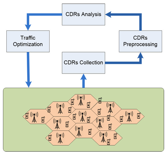
Figure 17.
Demonstration of CDRs driven framework.
In the proposed optimization framework, CDR collection and traffic optimization are online processes that directly interact with the network infrastructure continuously. While CDR preprocessing and analysis are offline processes that start a certain time period (a parameter decided based on density and activity levels in the cluster), apply proposed technique on CDR data from the inactivity period, predict network activity for the next quantum and suggest fresh network parameters to the traffic optimizer. Thus, the proposed method uses unsupervised machine learning to extract spatiotemporal features to prepare training data set for the supervised learning algorithm that actually tags the activity levels based on spatial and temporal features.
7. Conclusions and Future Direction
This article elaborates the potential benefits of CDR data analytics in mobile networks. Our work provides an effective spatiotemporal analysis approach to understand and monitor the mobile traffic patterns of large scale city. Experimental results show that the useful insights extracted from CDR data would be very helpful in optimizing mobile network resources. These findings help to understand the spatial and temporal dynamics of the traffic pattern in a comprehensive way. The framework for optimizing network traffic is built on the basis of insights obtained from CDR data analytics. Thus, we believe our classification framework for mobile traffic partitioning is enhanced network performance and QoS requirements.
The useful insights obtained from spatiotemporal analytics of CDRs are helpful in subscribers’ behavior profiling, resources consumption profiling, and mobility profiling. These useful insights will perform a key role in policy making and the provision of services for the implementation of smart cities and urban computing.
Author Contributions
Conceptualization, K.S. and A.A.; Methodology, K.S. and A.A.; Resources, H.A. and Z.Z.; Writing—Original Draft Preparation, K.S. and H.A.; Writing—Review & Editing, K.S., H.A., A.A. and Z.Z.; Supervision, H.A. and Z.Z.; Funding Acquisition, Z.Z.
Funding
This work was supported in part by the Key Project of the National Natural Science Foundation of China under Grant 61431001, in part by the Beijing Natural Science Foundation under Grant L172026, in part by the Key Laboratory of Cognitive Radio and Information Processing, Ministry of Education, Guilin University of Electronic Technology.
Conflicts of Interest
The authors declares that there is no conflict of interest regarding the publication of this article.
References
- Ericsson. More than 50 Billion Connected Devices; Ericsson: Stockholm, Sweden, 2011. [Google Scholar]
- Sultan, K.; Ali, H.; Zhang, Z. Big Data Perspective and Challenges in Next Generation Networks. Future Internet 2018, 10, 56. [Google Scholar] [CrossRef]
- Cisco VNI Mobile. Cisco Visual Networking Index: Global Mobile Data Traffic Forecast Update, 2010–2015 White Paper; Cisco: San Jose, CA, USA, 2011; Retrieved February 2011. [Google Scholar]
- Das, A.K.; Pathak, P.H.; Chuah, C.; Mohapatra, P. Contextual localization through network traffic analysis. In Proceedings of the IEEE INFOCOM 2014 IEEE Conference on Computer Communications, Toronto, ON, Canada, 27 April–2 May 2014; pp. 925–933. [Google Scholar]
- Dong, Y.; Yang, Y.; Tang, J.; Yang, Y.; Chawla, N.V. Inferring user demographics and social strategies in mobile social networks. In Proceedings of the 20th ACM SIGKDD International Conference on Knowledge Discovery and Data Mining, New York, NY, USA, 24–27 August 2014; pp. 15–24. [Google Scholar]
- Shafiq, M.Z.; Ji, L.; Liu, A.X.; Pang, J.; Wang, J. Characterizing geospatial dynamics of application usage in a 3G cellular data network. In Proceedings of the INFOCOM, Orlando, FL, USA, 25–30 March 2012; pp. 1341–1349. [Google Scholar]
- Bao, Y.; Wu, H.; Liu, X. From prediction to action: Improving user experience with data-driven resource allocation. IEEE J. Sel. Areas Commun. 2017, 35, 1062–1075. [Google Scholar] [CrossRef]
- Gill, P.; Arlitt, M.; Li, Z.; Mahanti, A. Youtube traffic characterization: A view from the edge. In Proceedings of the 7th ACM SIGCOMM Conference on Internet Measurement, San Diego, CA, USA, 24–26 October 2007; pp. 15–28. [Google Scholar]
- Cao, J.; Cleveland, W.S.; Gao, Y.; Jeffay, K.; Smith, F.D.; Weigle, M. Stochastic models for generating synthetic HTTP source traffic. In Proceedings of the INFOCOM 2004, Twenty-third Annual Joint Conference of the IEEE Computer and Communications Societies, Hong Kong, China, 7–11 March 2004; pp. 1546–1557. [Google Scholar]
- Willkomm, D.; Machiraju, S.; Bolot, J.; Wolisz, A. Primary users in cellular networks: A large-scale measurement study. In Proceedings of the 2008 3rd IEEE Symposium on New Frontiers in Dynamic Spectrum Access Networks, Chicago, IL, USA, 14–17 October 2008; pp. 1–11. [Google Scholar]
- Zerfos, P.; Meng, X.; Wong, S.H.Y.; Samanta, V.; Lu, S. A study of the short message service of a nationwide cellular network. In Proceedings of the 6th ACM SIGCOMM Conference on Internet Measurement, Rio de Janeriro, Brazil, 25–27 October 2006; pp. 263–268. [Google Scholar]
- Noulas, A.; Mascolo, C.; Frias-Martinez, E. Exploiting foursquare and cellular data to infer user activity in urban environments. In Proceedings of the 2013 IEEE 14th International Conference on Mobile Data Management (MDM), Milan, Italy, 3–6 June 2013; pp. 167–176. [Google Scholar]
- Li, Y.; Peng, C.; Yuan, Z.; Li, J.; Deng, H.; Wang, T. Mobileinsight: Extracting and analyzing cellular network information on smartphones. In Proceedings of the 22nd Annual International Conference on Mobile Computing and Networking, New York, NY, USA, 3–7 October 2016; pp. 202–215. [Google Scholar]
- Jin, Y.; Duffield, N.; Gerber, A.; Haffner, P.; Hsu, W.L.; Jacobson, G.; Sen, S.; Venkataraman, S.; Zhang, Z.L. Characterizing data usage patterns in a large cellular network. In Proceedings of the 2012 ACM SIGCOMM workshop on Cellular networks: Operations, Challenges, and Future Design, Helsinki, Finland, 13 August 2012; pp. 7–12. [Google Scholar]
- Zhang, Y.; Arvidsson, A. Understanding the characteristics of cellular data traffic. In Proceedings of the 2012 ACM SIGCOMM Workshop on Cellular Networks: Operations, Challenges, and Future Design, Helsinki, Finland, 13 August 2012; pp. 13–18. [Google Scholar]
- Kosinski, M.; Stillwell, D.; Graepel, T. Private traits and attributes are predictable from digital records of human behavior. Proc. Natl. Acad. Sci. USA 2013, 110, 5802–5805. [Google Scholar] [CrossRef] [PubMed]
- Laurila, J.K.; Gatica-Perez, D.; Aad, I.; Bornet, O.; Do, T.M.; Dousse, O.; Eberle, J.; Miettinen, M. The mobile data challenge: Big data for mobile computing research. In Proceedings of the 10th International Conference on Pervasive Computing, Pervasive 2012, Newcastle, UK, 18–22 June 2012. [Google Scholar]
- Deville, P.; Linard, C.; Martin, S.; Gilbert, M.; Stevens, F.R.; Gaughan, A.E.; Blondel, V.D.; Tatem, A.J. Dynamic population mapping using mobile phone data. Proc. Natl. Acad. Sci. USA 2014, 111, 15888–15893. [Google Scholar] [CrossRef] [PubMed]
- Ficek, M.; Kencl, L. Inter-call mobility model: A spatio-temporal refinement of call data records using a gaussian mixture model. In Proceedings of the 2012 IEEE INFOCOM, Orlando, FL, USA, 25–30 March 2012; pp. 469–477. [Google Scholar]
- Simini, F.; González, M.C.; Maritan, A.; Barabási, A.L. A universal model for mobility and migration patterns. Nature 2012, 484, 96. [Google Scholar] [CrossRef] [PubMed]
- Song, C.; Koren, T.; Wang, P.; Barabási, A.-L. Modelling the scaling properties of human mobility. Nat. Phys. 2010, 6, 818. [Google Scholar] [CrossRef]
- Song, C.; Qu, Z.; Blumm, N.; Barabási, A. Limits of predictability in human mobility. Sci. Am. Assoc. Adv. Sci. 2010, 327, 1018–1021. [Google Scholar] [CrossRef] [PubMed]
- Gonzalez, M.C.; Hidalgo, C.A.; Barabasi, A.-L. Understanding individual human mobility patterns. Nature 2008, 443, 779. [Google Scholar] [CrossRef] [PubMed]
- Lee, D.; Zhou, S.; Zhong, X.; Niu, Z.; Zhou, X.; Zhang, H. Spatial modeling of the traffic density in cellular networks. IEEE Wirel. Commun. 2014, 21, 80–88. [Google Scholar] [CrossRef]
- Wang, H.; Ding, J.; Li, Y.; Hui, P.; Yuan, J.; Jin, D. Characterizing the spatio-temporal inhomogeneity of mobile traffic in large-scale cellular data networks. In Proceedings of the 7th International Workshop on Hot Topics in Planet-scale mObile computing and online Social neTworking, Hangzhou, China, 22 June 2015; pp. 19–24. [Google Scholar]
- Sultan, K.; Ali, H.; Zhang, Z. Call Detail Records Driven Anomaly Detection and Traffic Prediction in Mobile Cellular Networks. IEEE Access 2018, 6, 41728–41737. [Google Scholar] [CrossRef]
- Dandelion API. Available online: https://dandelion.eu (accessed on 31 January 2015).
- Zhang, C.; Zhang, H.; Yuan, D.; Zhang, M. Citywide Cellular Traffic Predictin Based on Densely Connected Convolutional Neural Networks. IEEE Commun. Lett. 2018, 22, 1656–1659. [Google Scholar] [CrossRef]
- Jason, B. Introduction to Time Series Forecasting With Python; Machine Learning Mastery: Vermont, Australia, 2017. [Google Scholar]
- Wang, J.; Wu, Y.; Yen, N.; Guo, S.; Cheng, Z. Big data analytics for emergency communication networks: A survey. IEEE Commun. Surv. Tutorials 2016, 18, 1758–1778. [Google Scholar] [CrossRef]
- Huang, S.; Liu, Q.; Han, T.; Ansari, N. Data-Driven Network Optimization in Ultra-Dense Radio Access Networks. In Proceedings of the 2017 IEEE Global Communications Conference, GLOBECOM 2017, Singapore, 4–8 December 2017; pp. 1–6. [Google Scholar]
- Rafique, D.; Velasco, L. Machine learning for network automation: Overview, architecture, and applications [invited tutorial]. OSA/IEEE J. Opt. Commun. Netw. 2018, 10, D126–D148. [Google Scholar] [CrossRef]
- Fan, B.; Leng, S.; Yang, K. A dynamic bandwidth allocation algorithm in mobile networks with big data of users and networks. IEEE Netw. 2016, 30, 6–10. [Google Scholar] [CrossRef]
- Zheng, K.; Yang, Z.; Zhang, K.; Chatzimisios, P.; Yang, K.; Xiang, W. Big data-driven optimization for mobile networks toward 5G. IEEE Netw. 2016, 30, 44–51. [Google Scholar] [CrossRef]
- Zoha, A.; Saeed, A.; Farooq, H.; Rizwan, A.; Imran, A.; Imran, M.A. Leveraging Intelligence from Network CDR Data for Interference aware Energy Consumption Minimization. IEEE Trans. Mob. Comput. 2018, 17, 1569–1582. [Google Scholar] [CrossRef]
© 2019 by the authors. Licensee MDPI, Basel, Switzerland. This article is an open access article distributed under the terms and conditions of the Creative Commons Attribution (CC BY) license (http://creativecommons.org/licenses/by/4.0/).