Mutual Information, the Linear Prediction Model, and CELP Voice Codecs

Abstract

We write the mutual information between an input speech utterance and its reconstruction by a code-excited linear prediction (CELP) codec in terms of the mutual information between the input speech and the contributions due to the short-term predictor, the adaptive codebook, and the fixed codebook. We then show that a recently introduced quantity, the log ratio of entropy powers, can be used to estimate these mutual informations in terms of bits/sample. A key result is that for many common distributions and for Gaussian autoregressive processes, the entropy powers in the ratio can be replaced by the corresponding minimum mean squared errors. We provide examples of estimating CELP codec performance using the new results and compare these to the performance of the adaptive multirate (AMR) codec and other CELP codecs. Similar to rate distortion theory, this method only needs the input source model and the appropriate distortion measure.

1. Introduction

Voice coding is a critical technology for digital cellular communications, voice over Internet protocol (VoIP), voice response applications, and videoconferencing systems [1,2]. Code-excited linear prediction (CELP) is the most widely deployed method for speech coding today, serving as the primary speech coding method in the adaptive multirate (AMR) codec [3] and in the more recent enhanced voice services (EVS) codec [4], both of which are used in cell phones and VoIP. At a high level, a CELP codec consists of a linear prediction model excited by an adaptive codebook and a fixed codebook. The linear prediction model captures the vocal tract dynamics (short-term memory) and the adaptive codebook folds in the long-term periodicity due to speaker pitch. The fixed codebook tries to represent the excitation for unvoiced speech and any remaining excitation energy not modeled by the adaptive codebook [2,5].

The encoder uses an analysis-by-synthesis paradigm to select the best fixed codebook excitation based on minimizing a frequency-weighted perceptual error signal. However, the linear prediction coefficients and the long-term predictor parameters are calculated to minimize the unweighted mean squared error and then substituted into the codec structure prior to the analysis-by-synthesis optimization.

No characterization of the relative contributions of the several CELP codec components to the overall CELP codec perceptual performance is known. That is, given a segment of an input speech signal, what is the relative importance of the short-term predictor, the long-term predictor, and the fixed codebook to the perceptual quality achieved by the CELP codec? The mean squared prediction error can be calculated for the first two, and a translation of mean squared error to perceptual quality has been devised for calculating rate distortion bounds for speech coders in Gibson and Hu [6]. An indication of the relative reduction in bits/sample provided by each component for a given quality would be very useful in optimizing codec performance and for investigating new adaptive codec structures.

In this paper, we develop and extend an approach suggested by Gibson [5] and decompose the mutual information between the input speech and the speech reconstructed by a CELP codec into the sum of unconditional and conditional mutual informations between the input speech and the linear prediction component, the adaptive codebook, and the fixed codebook, and show that this decomposition can be used to predict CELP codec performance based upon analyzing the input speech utterance, without actually implementing the CELP codec and processing the speech. We present examples comparing the estimated CELP codec performance and the actual performance achieved by CELP codecs. The approach is highly novel and the agreement between the actual and estimated performance is surprising.

The paper is outlined as follows. Section 2 provides an overview of the principles of Code-Excited Linear Prediction (CELP) needed for the remainder of the paper, while Section 3 develops the decomposition of the mutual information between the input speech and the speech reconstructed by the CELP codec. The concept of entropy power as defined by Shannon [7] is presented in Section 4, and the ordering of mutual information as a signal is passed through a cascaded signal processing system is stated in Section 5. The recently proposed quantity, the log ratio of entropy powers, is given in Section 6, where it is shown that the mean squared estimation errors can be substituted for the entropy powers in the ratio for an important set of probability densities [5,8,9]. The mutual information between the input speech and the short-term prediction sequence is discussed in Section 7 and the mutual information provided by the adaptive and fixed codebooks about the input speech is developed in Section 8. The promised analysis of CELP codecs using these prior mutual information results based on only the input speech model and the distortion measure is presented in Section 9. Section 10 contains conclusions drawn from the results in the paper.

2. Code-Excited Linear Prediction (CELP)

Block diagrams of a code-excited linear prediction (CELP) encoder and decoder are shown in Figure 1 and Figure 2, respectively [1,2].

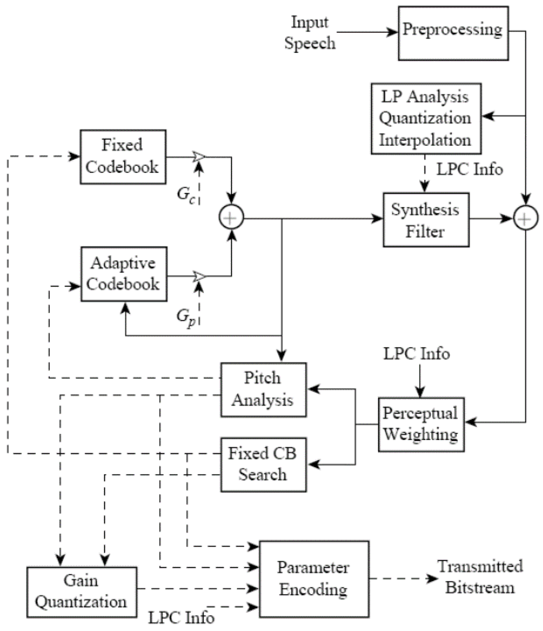
We provide a brief description of the various blocks in Figure 1 and Figure 2 to begin. The CELP encoder is an implementation of the Analysis-by-Synthesis (AbS) paradigm [1]. CELP, like most speech codecs in the last 45 years, is based on the linear prediction model for speech, wherein the speech is modeled as

$$s(k)=\sum _{i=1}^N{a}_{i}s(k-i)+Gw(k),$$

(1)

where we see that the current speech sample at time instant k is represented as a weighted linear combination of N prior speech samples plus an excitation term at the current time instant. The weights, $a_i,i=1,2,\dots ,N$, are called the linear prediction coefficients. The synthesis filter in Figure 1 has the form of this linear combination of past outputs and the fixed and adaptive codebooks model the excitation, $w(k)$. The LP analysis block calculates the linear prediction coefficients, and we see that the block also quantizes the coefficients so that encoder and decoder use exactly the same coefficients.

The adaptive codebook is used to capture the long-term memory due to the speaker pitch and the fixed codebook is selected to be an algebraic codebook, which has mostly zero values and only a relatively few nonzero pulses. The pitch analysis block calculates the adaptive codebook long-term memory. The process is AbS in that for a block of (say) M input speech samples, the linear prediction coefficients and long-term memory are calculated and a perceptual weighting filter is constructed using the linear prediction coefficients. Then, for every length M sequence (codevector) in the fixed codebook, (say) there are L code vectors in the fixed codebook, a synthesized sequence of speech samples are produced. This is the fixed codebook search block. The best codevector out of the L in the fixed codebook in terms of the length M synthesized sequence that best matches the input block of length M based on minimizing the perceptually weighted squared error is chosen and transmitted to the CELP decoder along with the long-term memory, the predictor coefficients, and the codebook gains. These operations are represented by the parameter encoding block in Figure 1 [1,10].

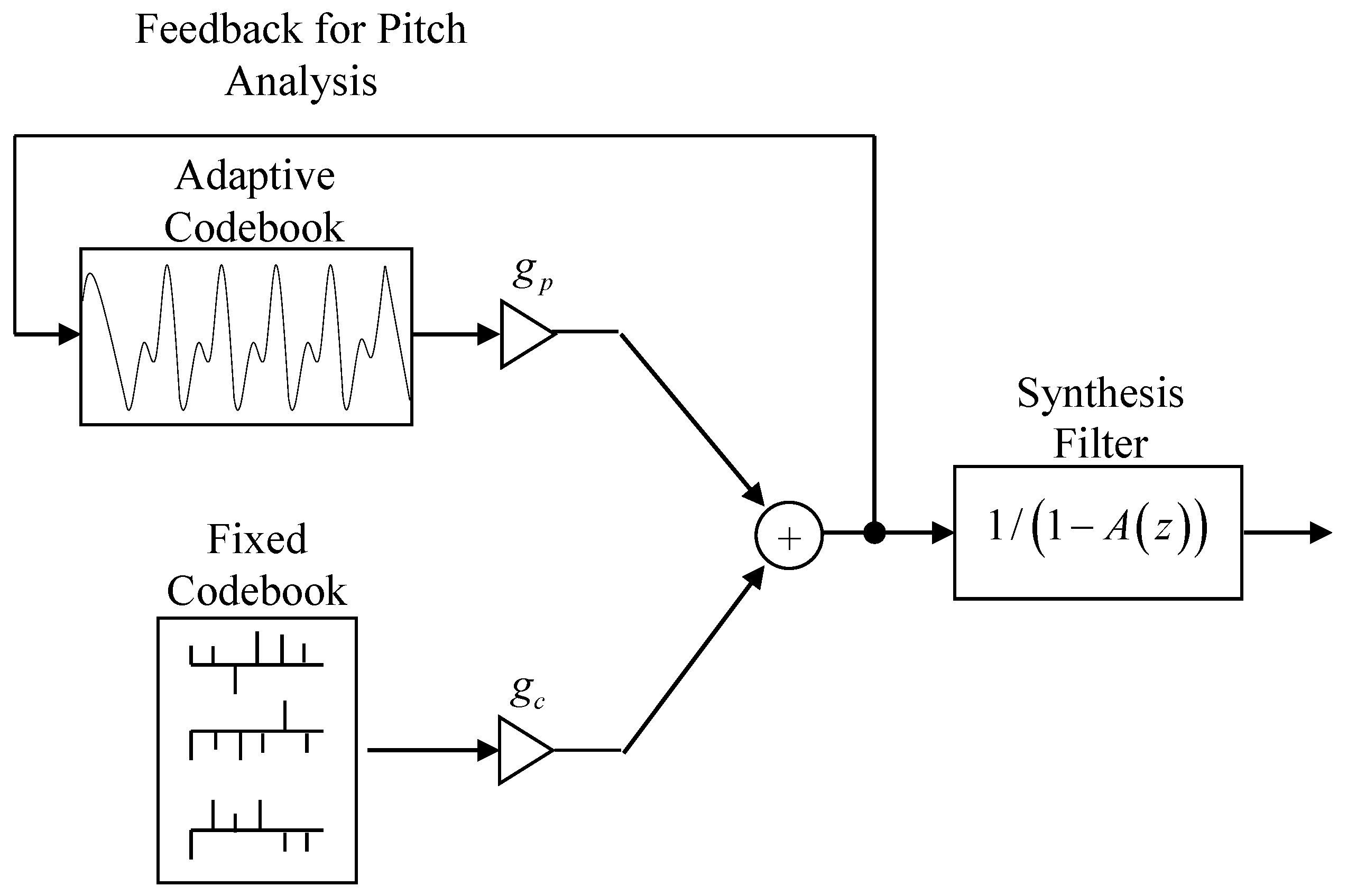
The CELP decoder uses these parameters to synthesize the block of M reconstructed speech samples presented to the listener as shown in Figure 2. There is also post-processing, which is not shown in the figure.

The quality and intelligibility of the synthesized speech is often determined by listening tests that produce mean opinion scores (MOS), which for narrowband speech vary from 1 up to 5 [11,12]. A well-known codec such as G.711 is usually included to provide an anchor score value with respect to which other narrowband codecs can be evaluated [13,14,15].

It would be helpful to be able to associate a separate contribution to the overall performance by each of the main components in Figure 2, namely the fixed codebook, the adaptive codebook, and the synthesis filter. Signal to quantization noise ratio (SNR) is often used for speech waveform codecs, but CELP does not attempt to follow the speech waveform, so SNR is not applicable. One characteristic of CELP codecs that is well known is that those speech attributes not captured by the short-term predictor must be accounted for, as best as possible, by the excitation codebooks, but an objectively meaningful measure of the individual component contributions is yet to be advanced.

In the next section, we propose a decomposition in terms of the mutual information and conditional mutual information with respect to the input speech provided by each component in the CELP structure, that appears particularly useful and interesting for capturing the performance and the trade-offs involved.

3. A Mutual Information Decomposition

Gibson [5] proposed the following decomposition of the several contributions to the synthesized speech by the CELP codec components. In particular, letting X represent a frame of input speech samples, we define $X_R$, $X_N$, and $X_C$ as the reconstructed speech, the prediction component, and the combined fixed and adaptive codebook components, respectively. Then we can write the mutual information between the input speech and the reconstructed speech as

$$I(X;X_R)=I(X;X_N,X_C)=I(X;X_N)+I(X;X_C|X_N).$$

(2)

This expression states that the mutual information between the original speech X and the reconstructed speech $X_R$ equals the mutual information between X and $X_N$, the Nth order linear prediction of X, plus the mutual information between X and the combined codebook excitations $X_C$ conditioned on $X_N$. Thus, to achieve or maintain a specified mutual information between the original speech and the reconstructed speech, any change in $X_N$ must be offset by an adjustment of $X_C$. This fits what is known experimentally and was alluded to earlier. If we define $X_A$ to represent the adaptive codebook contribution and $X_F$ to represent the fixed codebook contribution, we can further decompose $I(X;X_C|X_N)$ as

$$\begin{array}{cc}\hfill I(X;X_C|X_N)=& I(X;X_A,X_F|X_N)\hfill \\ \hfill =& I(X;X_A|X_N)+I(X;X_F|X_N,X_A),\hfill \end{array}$$

(3)

where we have used the chain rule for mutual information [16]. The expressions in Equations (2) and (3) correspond to the analysis chain illustrated in Figure 3, so $X\to X_N\to X_A\to X_F$. $A(z)$ in Figure 3 represents the short-term prediction component as in Equation (1), and $P(z)$ is the long-term predictor as discussed later in Section 8.1.

We can also write a chain rule mutual information expression for the synthesis chain in Figure 4 as

$$\begin{array}{cc}\hfill I(X;X_R)=& I(X;X_C)+I(X;X_N|X_C)\hfill \\ \hfill =& I(X;X_A,X_F)+I(X;X_N|X_C)\hfill \\ \hfill =& I(X;X_F)+I(X;X_A|X_F)+I(X;X_N|X_A,X_F),\hfill \end{array}$$

(4)

so $X_F\to X_A\to X_N\to X$.

Notice that we are not attempting to model the mutual informations in the CELP encoder and decoder of Figure 1 and Figure 2 directly; we are effectively creating analysis and synthesis Markov chains that use the choices for $X_F,X_A,X_N$ produced by the CELP encoder in the original analysis-by-synthesis CELP structure prior to the adoption of the adaptive codebook approximation [17].

While these expressions in Equations (2)–(4) are interesting, the challenge that remains is to characterize each of these mutual informations without actually having to calculate them directly from data, which is a difficult problem in and of itself [18].

An interesting quantity introduced and analyzed by Gibson in a series of papers is the log ratio of entropy powers [5,8,9]. Specifically, the log ratio of entropy powers is related to the difference in mutual information, and further, in many cases, the entropy powers can be replaced with the minimum mean squared prediction error (MMSPE) in the ratio. Using the MMSPE, the difference in mutual informations can be easily calculated. The following sections develop these concepts before we apply them to an analysis of the CELP structure.

4. Entropy Power/Entropy Rate Power

Given a random variable X with probability density function $p(x)$, we can write the differential entropy $h(X)=-{\int }_{-\infty }^{\infty }p(x)logp(x)dx$, where the variance $var(X)={\sigma }^2$. Since the Gaussian distribution has the maximum differential entropy of any distribution with mean zero and variance ${\sigma }^2$ [16],

$$h(X)\le \frac{1}{2}log2\pi e{\sigma }^2,$$

(5)

from which we obtain

$$Q=\frac{1}{(2\pi e)}exp2h(X)\le {\sigma }^2,$$

(6)

where Q was defined by Shannon to be the entropy power associated with the differential entropy of the original random variable [7]. In addition to defining entropy power, this equation shows that the entropy power is the minimum variance that can be associated with the not-necessarily-Gaussian differential entropy $h(X)$.

5. Cascaded Signal Processing

Figure 5 shows a cascade of N signal processing operations with the estimator blocks at the output of each stage as studied by Messerschmitt [19]. He used the conditional mean at each stage and the corresponding conditional mean squared errors to obtain a representation of the distortion contributed by each stage. We analyze the cascade connection in terms of information theoretic quantities, such as mutual information, differential entropy, and entropy rate power. Similar to Messerschmitt, we consider systems that have no hidden connections between stages other than those explicitly shown. Therefore, we conclude directly from the data processing inequality [16] that

$$I(X;Y_1)\ge \dots \ge I(X;Y_{N-1})\ge I(X;Y_N)\ge I(X;\widehat{X}).$$

(7)

Since $I(X;Y_n)=h(X)-h(X|Y_n)$, it follows from Equation (7) that for non-negative $h(·)$,

$$h(X|Y_1)\le \dots \le h(X|Y_{N-1})\le h(X|Y_N)\le h(X).$$

(8)

For the optimal estimators at each stage, the basic data processing inequality also yields $I(X;Y_n)\ge I(X;{\widehat{X}}_n)$, and thus $h(X|Y_n)\le h(X|{\widehat{X}}_n)$.

These are the fundamental results, that additional processing cannot increase the mutual information.

Now we notice that the series of inequalities in Equation (8) along with the entropy power expression in Equation (6) gives us the series of inequalities in terms of entropy power at each stage in the cascaded signal processing operations:

$$Q_{X|Y_1}\le \dots \le Q_{X|Y_{N-1}}\le Q_{X|Y_N}\le Q_X.$$

(9)

We can also write that

$$Q_{X|Y_n}\le Q_{X|{\widehat{X}}_n}.$$

(10)

In the context of Equation (9), the notation $Q_{X|Y_n}$ denotes the minimum variance when reconstructing an approximation to X given the sequence at the output of stage n in the chain [8].

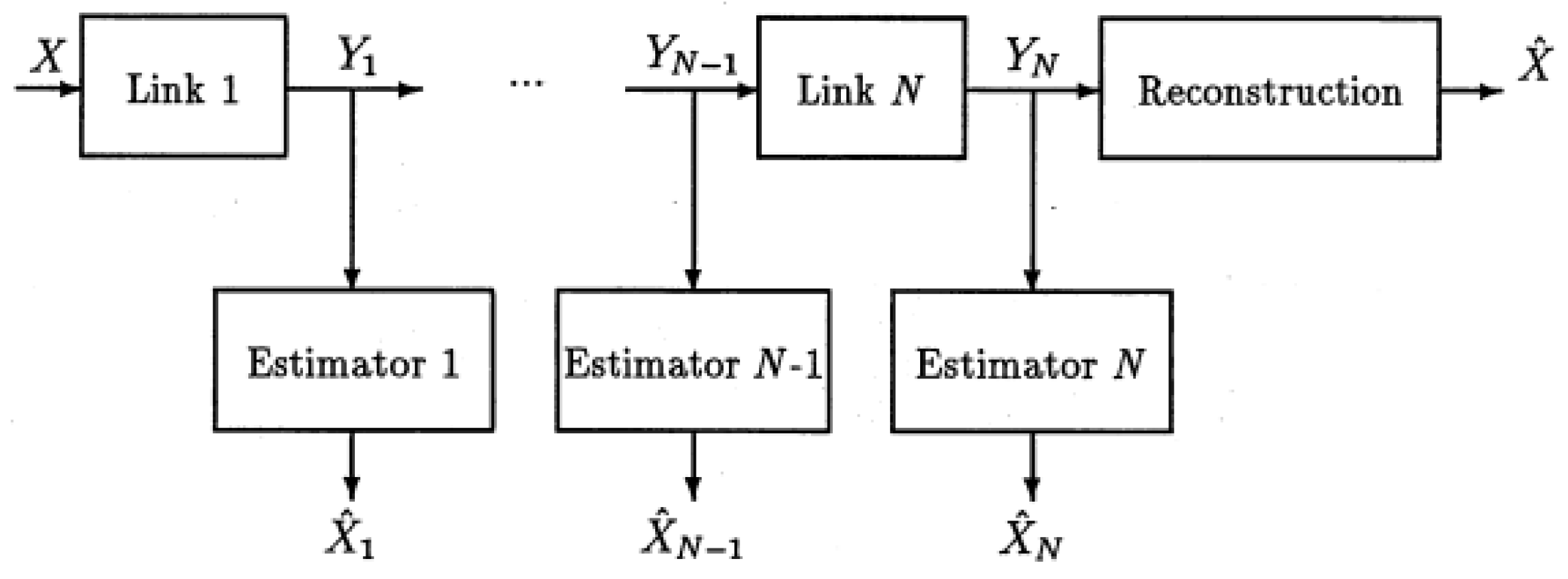
6. Log Ratio of Entropy Powers

We can use the definition of the entropy power in Equation (6) to express the logarithm of the ratio of two entropy powers in terms of their respective differential entropies as [8]

$$log\frac{Q_X}{Q_Y}=2[h(X)-h(Y)].$$

(11)

We can write a conditional version of Equation (6) as

$$Q_{X|Y_n}=\frac{1}{(2\pi e)}exp2h(X|Y_n)\le Var(X|Y_n),$$

(12)

and from which we can express Equation (11) in terms of the entropy powers at successive stages in the signal processing chain (Figure 5), as

$$\frac{1}{2}log\frac{Q_{X|Y_n}}{Q_{X|Y_{n-1}}}=h(X|Y_n)-h(X|Y_{n-1}).$$

(13)

If we add and subtract $h(X)$ to the right-hand side of Equation (13), we then obtain an expression in terms of the difference in mutual information between the two stages as

$$\frac{1}{2}log\frac{Q_{X|Y_n}}{Q_{X|Y_{n-1}}}=I(X;Y_{n-1})-I(X;Y_n).$$

(14)

From the series of inequalities on the entropy power in Equation (9), we know that both expressions in Equations (13) and (17) are greater than or equal to zero.

These results are from [8] and extend the data processing inequality by providing a new characterization of the information loss between stages in terms of the entropy powers of the two stages. Since differential entropies are difficult to calculate, it would be particularly useful if we could obtain expressions for the entropy power at two stages and then use Equations (13) and (17) to find the difference in differential entropy and mutual information between these stages.

We are interested in studying the change in the differential entropy and mutual information brought on by different signal processing operations by investigating the log ratio of entropy powers.

In the following, we highlight several cases where Equation (11) holds with equality when the entropy powers are replaced by the corresponding variances. The Gaussian and Laplacian distributions often appear in studies of speech processing and other signal processing applications [10,15,20], so we show that substituting the variances for entropy powers in the log ratio of entropy powers for these distributions satisfies Equation (11) exactly. For two i.i.d. Gaussian distributions with zero mean and variances ${\sigma }_X^2$ and ${\sigma }_Y^2$, we have directly that $Q_X={\sigma }_X^2$ and $Q_Y={\sigma }_Y^2$, so

$$\frac{1}{2}log\frac{Q_X}{Q_Y}=\frac{1}{2}log\frac{{\sigma }_X^2}{{\sigma }_Y^2}=[h(X)-h(Y)],$$

(15)

which satisfies Equation (11) exactly. Of course, since the Gaussian distribution is the basis for the definition of entropy power, this result is not surprising.

For two i.i.d. Laplacian distributions with variances ${\lambda }_X^2$ and ${\lambda }_Y^2$ [21], their corresponding entropy powers $Q_X=2e{\lambda }_X^2/\pi$ and $Q_Y=2e{\lambda }_Y^2/\pi$, respectively, so we form

$$\begin{array}{cc}\hfill \frac{1}{2}log\frac{Q_X}{Q_Y}=& \frac{1}{2}log\frac{{\lambda }_X^2}{{\lambda }_Y^2}\hfill \\ \hfill =& [h(X)-h(Y)].\hfill \end{array}$$

(16)

Since $h(X)=ln(2e{\lambda }_X)$, the Laplacian distribution also satisfies Equation (11) exactly [5]. We thus conclude that we can substitute the variance, or for zero mean Laplacian distributions, the mean squared value for the entropy power, in Equation (11), and the result is the difference in differential entropies.

Interestingly, using mean squared errors or variances in Equation (11) is accurate for many other distributions as well. It is straightforward to show that Equation (11) holds with equality when the entropy powers are replaced by mean squared error for the logistic, uniform, and triangular distributions as well. Furthermore, the entropy powers can be replaced by the ratio of the squared parameters for the Cauchy distribution.

Therefore, the satisfaction of Equation (11) with equality occurs in more than one or two special cases. The key points are first that the entropy power is the smallest variance that can be associated with a given differential entropy, so the entropy power is some fraction of the mean squared error for a given differential entropy. Second, Equation (11) utilizes the ratio of two entropy powers, and thus, if the distributions corresponding to the entropy powers in the ratio are the same, the scaling constant (fraction) multiplying the two variances will cancel out. Therefore, we are not saying that the mean squared errors equal the entropy powers in any case but for Gaussian distributions. It is the new quantity, the log ratio of entropy powers, that enables the use of the mean squared error to calculate the loss in mutual information at each stage.

7. Mutual Information in the Short-Term Prediction Component

Gibson [5] used Equation (17) to investigate the change in mutual information as the predictor order, denoted in the following by N, is increased for different speech frames. Based on several analyses of the MMSPE and the fact that the log ratio of entropy powers can be replaced with the log ratio of MMSPEs for several different distributions, as outlined in Section 6 and in [9], we can use the expression

$$\frac{1}{2}log\frac{MMSPE(X,X_{N-1})}{MMSPE(X,X_N)}=I(X;X_N)-I(X;X_{N-1}),$$

(17)

as in [5], to associate a change in mutual information with a change in the predictor order. Figure 6 (bottom) shows 160 time domain samples from a narrowband (200 to 3400 Hz) speech sentence sampled at 8000 samples/s, and the top plot is the magnitude of the spectral envelope calculated from the linear prediction model using Equation (1). We show the $MMSPE$ and the corresponding change in mutual information for predictor orders $N=1,2,\dots ,10$ in

Table 1. Change in mutual information from Equation (17) as the predictor order is increased: Frame 3237, $SPER=9.15$ dB; MMSPE, minimum mean squared prediction error.

N	$\mathit{MMSPE}(\mathit{X},{\mathit{X}}_{\mathit{N}})$	$\mathit{I}(\mathit{X};{\mathit{X}}_{\mathit{N}})-\mathit{I}(\mathit{X};{\mathit{X}}_{\mathit{N}-1})$
0	$1.0$	0 bits/letter
0–1	$0.402$	$0.656$ bits/letter
1–2	$0.328$	$0.147$ bits/letter
2–3	$0.294$	$0.0795$ bits/letter
3–4	$0.2465$	$0.125$ bits/letter
4–5	$0.239$	$0.0234$ bits/letter
5–6	$0.2117$	$0.0869$ bits/letter
6–7	$0.212$	$0.0$ bits/letter
7–8	$0.125$	$0.381$ bits/letter
8–9	$0.1216$	$0.0206$ bits/letter
9–10	$0.1216$	$0.0$ bits/letter
0–10 Total	$0.1216$	$1.52$ bits/letter

. Notice that the chain rule assumption indicated by Figure 5 is retained by the analysis chain in Figure 3 even as we increment N as in Equation (17) and in Table 1 if we use a lattice implementation of the prediction [15]. However, for most of our analyses in what follows, we consider fixed order predictors. From Table 1, we see that the mutual information between the input speech frame and a 10th order predictor is 1.52 bits/sample. We can examine the mutual information between the input speech and a 10th order linear predictor for other frames in the same speech utterance.

To categorize the differences in the speech frames for easy reference, we use a common indicator of predictor performance, the signal-to-prediction error (SPER) in dB [22], also called the prediction gain [15], defined as

$$SPER(dB)=10{log}_{10}\frac{MSE(X)}{MMSPE(X,X_{10})},$$

(18)

where $MSE(X)$ is the average energy in the utterance, and $MMSPE(X,X_{10})$ is the minimum mean squared prediction error achieved by a 10th order predictor. The $SPER$ can be calculated for any predictor order, but we choose $N=10$, a common choice in narrowband speech codecs and the predictor order that, on average, captures most of the possible reduction in mean squared prediction error without including long-term pitch prediction. For a normalized $MSE(X)=1.0$, we see that for the speech frame in Figure 6, the $SPER=9.15$ dB.

Several other speech frames by the same speaker are analyzed in [5], and the results for these frames are tabulated in

Table 2. Change in mutual information from Equation (17) for 10th order predictors and corresponding SPERs for several speech frames [5].

Speech Frame No.	$\mathit{SPER}$ in dB	$\mathit{I}(\mathit{X};{\mathit{X}}_{10})-\mathit{I}(\mathit{X};{\mathit{X}}_0)$
45	16	$2.647$ bits/letter
23	$11.85$	$1.968$ bits/letter
3314	$7.74$	$1.29$ bits/letter
87	5	$0.83$ bits/letter

. From this table, it is evident that the mutual information between the input speech and a 10th order linear predictor can change quite dramatically across frames, even with the same speaker. We observe that the change in mutual information in some sense mirrors a change in $SPER$, with a larger $SPER$ implying a larger mutual information. However, the explicit characterization in terms of mutual information is new and allows new analyses of the performance of CELP codecs in terms of bits/sample reduction in rate that can be associated with the short-term predictor. We provide this analysis in Section 9.

8. Mutual Information in the Fixed and Adaptive Codebooks

How do we find the change in mutual information provided by the adaptive codebook and the fixed codebook? The adaptive codebook relies on long-term prediction to model the vocal tract excitation due to the speaker pitch. As such, an approach similar to that used for the short-term or linear predictor is possible. The fixed codebook contribution in terms of bits/sample is less direct. We could attempt to estimate the codebook complexity, or we could simply use the number of bits/sample used to transmit the fixed codebook excitation. We elaborate on each of these in the following subsections.

8.1. Adaptive Codebook: Long-Term Prediction

The long-term predictor that makes up the adaptive codebook in CELP may have one or three taps and is of the form

$$P(z)={\beta }_{-1}{z}^{-(P-1)}+{\beta }_0{z}^{-P}+{\beta }_1{z}^{-(P+1)},$$

(19)

where ${\beta }_i,i=-1,0,1$, are the predictor coefficients that are updated on a frame-by-frame basis, and P is the lag of the periodic correlation that captures the pitch excitation of the vocal tract. A three-tap predictor as shown in Equation (19) requires a stability check to guarantee that this component does not cause divergence [23]. The single tap form given by

$$P(z)=\beta z^{-P}$$

(20)

only needs the stability check that $\left|\beta \right|<1$, which should hold for any normalized autocorrelation. The three-tap form can often provide improved performance over the single tap predictor, but at increased complexity.

We denote the long-term predicted value as $X_P^P$ to distinguish it from the short-term predictor of order N, $X_N$, which contains all terms up to and including N. Thus, we can write the MMSPE between X and $X_P^P$ as $MMSPE(X,X_P^P)$.

The prediction gain in dB is often used as a performance indicator for a pitch predictor. The long-term prediction gain has the form of Equation (18) but with $MMSPE(X,X_{10})$ replaced by $MMSPE(X,X_P^P)$, where $X_P^P$ is the long-term predicted value for a pitch lag of P samples, where usually $P=20$ up to $P=140$ samples at 8000 samples/s. Rather than calculate the prediction gain for selected speech frames, we consult the literature to get a range of values that might be expected.

Cuperman and Pettigrew [24] indicate a pitch prediction gain of 1 to 5 dB, but of around 2 dB on average. Other sources indicate that the prediction gains can be 3–4 dB [25] or up to 5–6 dB [26].

Table 3. Change in mutual information from Equation (17) for various pitch predictors and corresponding SPER.

$\mathit{SPER}$ in dB	$\mathit{I}(\mathit{X};{\mathit{X}}_{\mathit{P}}^{\mathit{P}})-\mathit{I}(\mathit{X};{\mathit{X}}_0)$
1	$0.1667$ bits/letter
2	$0.33$ bits/letter
3	$0.5$ bits/letter
4	$0.65$ bits/letter
6	$1.0$ bits/letter

shows the mutual information in bits/letter that can be associated with prediction gains of 1, 2, 3, 4, and 6 dB.

It is interesting to consult the standardized speech codecs to see how many bits/sample are allocated to coding the pitch gain (coefficient or coefficients) and the pitch delay (lag). For the narrowband form of the AMR codec, we see that for 7.95 bits/s rate, the pitch gain and pitch delay are allocated 16 and 28 bits, respectively, per 20 ms frame, or 44 bits/160 samples = 0.275 bits/sample [3]. For the highest rate of 12.2 kbits/s, pitch gain and delay are allocated 46 bits/160 samples = 0.2875 bits/sample. Consulting Table 3, we see that this corresponds to a $SPER$ of between 1 and 2 dB.

8.2. Fixed Codebook

The most often used fixed codebooks in popular speech coders are sparse and have several shifted phase tracks, where each track consists of equally spaced pulses with 4 or 5 zero values in between. The best codeword or excitation from the fixed codebook is then selected by searching these tracks in some specific order. Getting an estimate of the number of bits/sample to be associated with a fixed codebook is therefore challenging. However, we know a few specific things.

The initial studies of analysis-by-synthesis codecs used Gaussian random sequences as the excitation. In particular, Atal and Schroeder used 1024 Gaussian random sequences that were 40 samples long. Thus, this codebook used 10 bits/40 samples or 0.25 bits/sample [17]. However, this does not include the fixed codebook gain. The U.S. Federal Standard FS1016 CELP at 4.8 kbits/s has allocations of 56 bits per frame of 240 samples or 0.233 bits/sample to the fixed codebook [10]. For a CELP codec that operates at 6 kbits/s and above and a sparse codebook with five tracks and 8 pulses per track, an estimate of 3 bits plus a sign bit per track gives a fixed codebook rate of 0.5 bits/sample [25].

The narrowband AMR codec at 7.95 kbits/s allocates 88 bits/20 ms frame or 0.55 bits/sample to the fixed codebook, and at 12.2 kbits/s, 1 bit/sample is devoted to the fixed codebook gain and delay [3]. Thus, we see that at around 4 kbits/s the allocation is about 0.25 bits/sample, at 8 kbits/s the fixed codebook gets about 0.5 bits/sample, and at 12.2 kbits/s, 1 bit/sample.

We now have estimates of the bits/sample devoted to the short-term predictor, adaptive codebook, and fixed codebook for a CELP codec operating at different bit rates. In the following, we show how to exploit these estimates to predict the rate of CELP codecs for different speech sources.

9. Estimated versus Actual CELP Codec Performance

The analyses determining the mutual information in bits/sample between the input speech and the short-term linear prediction, the adaptive codebook, and the fixed codebook individually, are entirely new and provide new ways to analyze CELP codec performance by only analyzing the input source. In this section, we estimate the performance of a CELP codec by analyzing the input speech source to find the mutual information provided by each CELP component about the input speech and then subtract the three mutual informations from a reference codec rate in bits/sample for a chosen MOS value to get the final estimate of the rate required in bits/sample to achieve the target MOS.

For waveform speech coding, such as differential pulse code modulation (DPCM), for a particular utterance, we can study the rate in bits/sample versus the mean squared reconstruction error or SNR to obtain some idea of the codec performance for this input speech segment [14,15]. However, while SNR may order DPCM subjective codec performance correctly, it does not provide an indicator of the actual difference in subjective performance. Subjective performance is most accurately available by conducting subjective listening tests to obtain mean opinion scores (MOS). Alternatively, reasonable views of subjective performance can be obtained from software such as PESQ /MOS [12]. We use the latter. In either case, however, MOS cannot be generated on a per-frame basis as listening tests and PESQ values are generated from longer utterances.

Therefore, we cannot use the per-frame estimates of mutual information from Section 7 and need to calculate estimates of mutual information over longer sentences. To this end,

Table 4. Composite source models for narrowband speech sentences [6]. V, voiced; UV, unvoiced; ON, onset; H, hangover; S, silence.

Sequence	Mode	Autocorrelation Coefficients for V, ON, H	Mean Square	Probability
		Average Frame Energy for UV	Prediction Error
“lathe” (Female) (active speech level: $-18.1$ dBov) (sampling rate: 8 kHz)	V	[1 $0.8217$ $0.5592$ $0.3435$ $0.1498$ $0.0200$	0.0656	0.5265
		$-0.0517$$-0.0732$$-0.0912$$-0.1471$$-0.2340$]
	ON	[1 $0.8495$ $0.5962$ $0.3979$ $0.2518$]	$0.0432$	$0.0093$
	H	[1 $0.2709$ $0.2808$ $0.1576$ $0.1182$]	$0.7714$	$0.0186$
	UV	$0.1439$	$0.1439$	$0.0771$
	S			$0.3685$
“we were away” (Male) (active speech level: $-16.5$ dBov) (sampling rate: 8 kHz)	V	[1 $0.8014$ $0.5176$ $0.2647$ $0.0432$ $-0.1313$	0.0780	0.9842
		$-0.2203$$-0.3193$$-0.3934$$-0.4026$$-0.3628$]
	ON	[1 $0.8591$ $0.7215$ $0.6128$ $0.5183$]	$0.0680$	$0.0053$
	H			0
	UV			0
	S			$0.0105$

contains autocorrelations for two narrowband (200 to 3400 Hz) utterances sampled at 8000 samples/s, “We were away a year ago,” spoken by a male and “A lathe is a big tool. Grab every dish of sugar,” spoken by a female, including the decomposition of the sentences into five modes, namely voiced, unvoiced, onset, hangover, and silence, and their corresponding relative frequencies. The two utterances are taken from the Open Speech Repository [27]. These data are excerpted from tables in Gibson and Hu [6] and are not calculated on a per-frame basis but averaged over all samples of the utterance falling in the specified subsource model.

From Table 4, the voiced subsource models are set as $N=10$th order, with the 1 in the column vector representing the $a_0\mathrm{th}=1$ term. The onset and hangover modes are modeled as $N=4$th order autoregressive (AR). We see from this table that the sentence “We were away … ,” is voiced, with a relative frequency of 0.98, and that the sentence “A lathe is a big … ,” has a breakdown of voiced (0.5265), silence (0.3685), unvoiced (0.0771), onset (0.0093), and hangover (0.0186). The $MMSPEs$ for each mode are also shown in the table.

We focus on G.726 as our reference codec. Generally, G.726 adaptive differential pulse code modulation (ADPCM) at 32 kbits/s or 4 bits/sample for narrowband speech is considered to be “toll quality”. G.726 is selected as the reference codec because ADPCM is a waveform-following codec and is the best-performing speech codec that does not rely on a more sophisticated speech model. In particular, G.726 utilizes only two poles and six zeros, and the parameter adaptation algorithms rely only on polarities. G.726 will track pure tones as well as other temporal waveforms in addition to speech. In G.726, no parameters are coded and transmitted, only the quantized and coded prediction error signal. Finally, both mean squared reconstruction error or SNR and MOS have meaning for G.726, which is useful since SPER plays a role in estimating the change in mutual information from the log ratio of entropy powers.

From

Table 5. Codec rates to achieve PESQ/mean opinion score (MOS) of 4.0 for “We were away … ” [6]. AMR, adaptive multirate.

Codec	R Bits/Sample
G.726	$4.0$ bits/sample
G.729	$1.1$ bits/sample
AMR	$1.1$ bit/sample

and

Table 6. Codec rates to achieve PESQ/MOS of 4.0 for “Lathe” [6]. CNG, comfort noise generation.

Codec	R Bits/Sample
G.726	$4.0$ bits/sample
G.726 w/CNG	$2.8$ bits/sample
G.729	$1.0$ bits/sample
AMR	$1.0$ bit/sample

, G.726 achieves a PESQ/MOS of about 4.0 for 4 bits/sample and for both sentences, “We were away a year ago,” spoken by a male speaker and “A lathe is a big tool. Grab every dish of sugar,” spoken by a female [6]. Therefore, we use 4 bits/sample as our reference point for toll quality speech for these two sentences. We then subtract from the rate of 4 bits/sample the rates in bits/sample we associate with each of the CELP codec components as estimated from Section 7 and Section 8.

For “We were away … ,” we see from Table 4 that the 10th order model of the voiced mode has a $MMSPE=0.078$, which corresponds to a mutual information reduction of 1.84 bits/sample. For this highly voiced sentence, we estimate the mutual information corresponding to the adaptive codebook as 0.5 bits/sample, and at a codec rate of 8000 bits/s, the fixed codebook mutual information would correspond to 0.5 bits/sample. Silence corresponds to about only 1 percent of the total utterance. If we sum these contributions up and subtract them from 4 bits/sample, we obtain $4-2.84=1.16$ bits/sample. Inspecting Table 5, the rates for the AMR and G.729 codecs at this MOS are 1.1 bits/sample, so there is surprisingly good agreement.

From Table 4, we see that for the utterance, “A lathe is … ,” there is broader mix of speech modes, including significant silence and unvoiced components. Neither of these modes had to be dealt with for the sentence “We were away … ”. Since silence is almost never perfect silence and usually consists of low level background noise, we associate the bits/sample for silence with a silence detection/comfort noise generation (CNG) method [25]. From Table 6, we see that G.726 with CNG is about 1.2 bits/sample lower than G.726, even though it occurs for only a 0.3685 portion of the utterance. For the short-term prediction, the $MMSPE$ = 0.0656, which corresponds to a mutual information of 1.96 bits/sample. The adaptive codebook contribution at 8 kbits/s can again be estimated as 0.5 bits/sample, and the fixed codebook component estimated at 0.5 bits/sample.

If we now combine all of these estimates with their associated relative frequencies of occurrence as indicated in Table 4, we obtain a total mutual information of $0.5265(1.96+0.5)+1.2+0.5(0.0771)=2.5$ bits/sample. Subtracting this from 4 bits/sample, we estimate that the CELP codec rate in bits/sample for an MOS = 4.0 would be 1.5 bits/sample. We see from Table 6 that for AMR and G.729, their rate is 1.0 bits/sample. This gap can be narrowed if the adaptive codebook contribution is toward the upper end of the expected $SPER$ of say 6 dB. In this case, the voiced component has the mutual information of $0.5265(1.96+1.0)=1.56$, so the total mutual information is 2.8, and then subtracting from 4 bits/sample, we obtain a CELP codec rate estimate of 1.2 bits/sample to achieve an MOS = 4.0. The actual CELP rate needed by G.729 and AMR for this MOS is about 1.0 bits/sample, which constitutes good agreement.

10. Conclusions

We have introduced a new approach to estimating CELP codec performance on a particular speech utterance by analysis of the input speech source only. That is, a particular CELP codec does not need to be implemented and used to process the speech. We have presented examples that illustrate the steps in the process and the accuracy of the estimated performance. While the power of the approach is evident, it is clear that many more sentences need to be processed to gain experience in estimating the various components. However, this approach offers the possibility of conducting performance analyses prior to the implementation of new CELP codec architectures and perhaps other new speech codec designs. It is striking that estimates of codec performance are possible while only knowing the source model and the distortion measure. Thus, in one sense, this new method parallels rate distortion theory.

References

1. Chen, J.H.; Thyssen, J. Analysis-by-Synthesis Speech Coding. In Springer Handbook of Speech Processing; Springer: Berlin, Germany, 2008. [Google Scholar]
2. Gibson, J. Speech Compression. Information 2016, 7, 32. [Google Scholar] [CrossRef]
3. ETSI. 3GPP AMR Speech Codec; Transcoding Functions; Technical Report; ETSI: Sophia Antipolis, France, 2002. [Google Scholar]
4. Dietz, M.; Multrus, M.; Eksler, V.; Malenovsky, V.; Norvell, E.; Pobloth, H.; Miao, L.; Wang, Z.; Laaksonen, L.; Vasilache, A.; et al. Overview of the EVS codec architecture. In Proceedings of the 2015 IEEE International Conference on Acoustics, Speech and Signal Processing, Brisbane, Australia, 19–24 April 2015; pp. 5698–5702. [Google Scholar] [CrossRef]
5. Gibson, J.D. Entropy Power, Autoregressive Models, and Mutual Information. Entropy 2018, 20, 750. [Google Scholar] [CrossRef]
6. Gibson, J.D.; Hu, J. Rate distortion bounds for voice and video. Found. Trends. Commun. Inf. Theory 2014, 10, 379–514. [Google Scholar] [CrossRef]
7. Shannon, C.E. A mathematical theory of communication. Bell Syst. Technol. J. 1948, 27, 379–423. [Google Scholar] [CrossRef]
8. Gibson, J.D. Log Ratio of Entropy Powers. In UCSD Information Theory and Application Workshop; UCSD: La Jolla, CA, USA, 2018. [Google Scholar]
9. Gibson, J.; Oh, H. Analysis of Cascaded Signal Processing Operations Using Entropy Rate Power. In Proceedings of the 2018 52nd Asilomar Conference on Signals, Systems, and Computers, Pacific Grove, CA, USA, 28–31 October 2018. [Google Scholar]
10. Chu, W.C. Speech Coding Algorithms; Wiley: Hoboken, NJ, USA, 2003. [Google Scholar]
11. Grancharov, V.; Kleijn, W.B. Speech Quality Assessment. In Springer Handbook of Speech Proceessing; Springer: Berlin, Germany, 2008. [Google Scholar]
12. ITU-T Recommendation P.862. Perceptual Evaluation of Speech Quality (PESQ), an Objective Method for End-to-End Speech Quality Assessment of Narrow-Band Telephone Networks and Speech Codecs; ITU-T: Geneva, Switzerland, 2001. [Google Scholar]
13. Kleijn, W.B. Principles of Speech Coding. In Springer Handbook of Speech Proceessing; Springer: Berlin, Germany, 2008. [Google Scholar]
14. Gibson, J.D.; Berger, T.; Lookabaugh, T.; Lindbergh, D.; Baker, R.L. Digital Compression for Multimedia: Principles and Standards; Morgan Kaufmann Publishers Inc.: San Francisco, CA, USA, 1998. [Google Scholar]
15. Rabiner, L.R.; Schafer, R.W. Digital Processing of Speech Signals; Pearson: London, UK, 2011. [Google Scholar]
16. Cover, T.M.; Thomas, J.A. Elements of Information Theory; Wiley-Interscience: Hoboken, NJ, USA, 2006. [Google Scholar]
17. Schroeder, M.; Atal, B. Code-excited linear prediction(CELP): High-quality speech at very low bit rates. In Proceedings of the IEEE International Conference on Acoustics, Speech, and Signal Processing, Tampa, FL, USA, 26–29 April 1985; pp. 937–940. [Google Scholar] [CrossRef]
18. Darbellay, G.A.; Vajda, I. Estimation of the information by an adaptive partitioning of the observation space. IEEE Trans. Inf. Theory 1999, 45, 1315–1321. [Google Scholar] [CrossRef]
19. Messerschmitt, D.G. Accumulation of Distortion in tandem Communication links. IEEE Trans. Inf. Theory 1979, IT-25, 692–698. [Google Scholar] [CrossRef]
20. Gray, R.M. Linear Predictive Coding and the Internet Protocol; NOW: Hanover, MA, USA, 2010. [Google Scholar]
21. Shynk, J.J. Probability, Random Variables, and Random Processes: Theory and Signal Processing Applications; John Wiley & Sons: Hoboken, NJ, USA, 2012. [Google Scholar]
22. Sayood, K. Introduction to Data Compression; Morgan Kaufmann: Waltham, MA, USA, 2017. [Google Scholar]
23. Ramachandran, R.P.; Kabal, P. Pitch prediction filters in speech coding. IEEE Trans. Acoust. Speech Signal Process. 1989, 37, 467–478. [Google Scholar] [CrossRef]
24. Cuperman, V.; Pettigrew, R. Robust low-complexity backward adaptive pitch predictor for low-delay speech coding. Speech Vis. IEEE Proc. I Commun. 1991, 138, 338–344. [Google Scholar] [CrossRef]
25. Kondoz, A.M. Digital Speech: Coding for Low Bit Rate Communication Systems; Wiley: Hoboken, NJ, USA, 2004. [Google Scholar]
26. Kleijn, W.B.; Paliwal, K.K. Speech Coding and Synthesis; Elsevier: Amsterdam, The Netherlands, 1995. [Google Scholar]
27. Telchemy. Open Speech Repository. Available online: http://www.voiptroubleshooter.com/open_speech/index.html (accessed on 19 May 2019).
Figure 1. Code-excited linear prediction (CELP) encoder.
Information 10 00179 g001
Figure 2. CELP Decoder.
Information 10 00179 g002
Figure 3. Analysis chain.
Information 10 00179 g003
Figure 4. Synthesis chain.
Information 10 00179 g004
Figure 5. N-link system block diagram (adapted from [19]).
Information 10 00179 g005
Figure 6. Frame 3237 time domain waveform (bottom) and spectral envelope, signal-to-prediction error (SPER) = 9.15 dB.
Information 10 00179 g006