Abstract
Path planning, as the core of navigation control for mobile robots, has become the focus of research in the field of mobile robots. Various path planning algorithms have been recently proposed. In this paper, in view of the advantages and disadvantages of different path planning algorithms, a heuristic elastic particle swarm algorithm is proposed. Using the path planned by the A* algorithm in a large-scale grid for global guidance, the elastic particle swarm optimization algorithm uses a shrinking operation to determine the globally optimal path formed by locally optimal nodes so that the particles can converge to it rapidly. Furthermore, in the iterative process, the diversity of the particles is ensured by a rebound operation. Computer simulation and real experimental results show that the proposed algorithm not only overcomes the shortcomings of the A* algorithm, which cannot yield the shortest path, but also avoids the problem of failure to converge to the globally optimal path, owing to a lack of heuristic information. Additionally, the proposed algorithm maintains the simplicity and high efficiency of both the algorithms.
1. Introduction
Mobile robot path planning aims to allow a robot to identify a safe, collision-free path from a starting point to a target point in a given environment, for example, for intelligent security or industrial manufacturing [1,2,3]. Path planning is the core problem in mobile robot autonomous navigation. In recent years, it has become a prominent research topic in the field of mobile robotics. Many path planning algorithms are proposed [4,5,6,7], including grid methods, which include the A* algorithm based on an exact grid [8], and the probability grid method, based on an approximate grid [9,10]. Intelligent optimization algorithms, which are based on natural heuristics, are as follows: Neural network algorithms [11], genetic algorithms [12], ant colony algorithms [13], particle swarm optimization (PSO) [14,15,16], artificial bee colony algorithms [17,18], artificial potential field (APF) algorithms based on the virtual force field [19], the Voronoi graph method, and the tangent graph method, based on a cell structure [20,21]. Each of these algorithms has its own advantages and disadvantages. However, no single algorithm has been able to solve all the problems in path planning. Therefore, researchers attempt to improve the existing methods to overcome these issues.
The A* and PSO algorithms are simple and efficient for path planning. Improving the A* algorithm is primarily focused on overcoming the shortcoming that it does not yield the shortest path, owing to the effect of the grid resolution. Xin [22] proposes an improved A* algorithm that extends the eight neighbourhood propagation directions of the standard A* algorithm to infinity, thereby overcoming the disadvantage of the A* algorithm being constrained by the grid. Mac et al. [14] propose a global path planning method, for a moving robot, based on the optimization of multiple target particle groups in a chaotic environment. In this method, a geometric free configuration space of the robot was established by using the triangular decomposition method, and a non-collision path, as the input reference for the next level and was found by using the Dijkstra algorithm. Study [15] presents a type of motion path planning for an underwater robot, based on PSO. Since the local minimum value problem and inefficient path planning are easily caused by APFs, study [16] proposes an improved APF (PSO-TVAPF) based on the tangent vector method and PSO. The tangent vector obtained is generated at an angle that considers the gravitational force and repulsive force in the standard APF and then the driving force for the robot path planning is determined. To further improve the robustness of the algorithm and efficiency of the path planning, the APF based on the tangent vector (TVAPF) was optimized by using the particle swarm algorithm. The primary drawback of the PSO algorithm is the lack of heuristic information, causing it to easily fall into a local extremum. Hence, [23] combined PSO with the crossover and mutation mechanism of a genetic algorithm to maintain the diversity of the particles in the iterative process, such that the particles could converge to the global optimum. Ao et al. [24] make the inertial weight factor of the particles with poor fitness values in the iterative process zero, which reduces the invalid iterations of the algorithm. The convergence is further improved by analyzing the relationship between the acceleration factor and PSO convergence. Jiang et al. [25] propose an improved linear PSO algorithm with adaptive acceleration factors, which improve the convergence of the algorithm. Gong et al. [26] propose a hybrid of PSO and a genetic algorithm for path planning. To enhance the accuracy of path planning, study [27] first improves the standard particle swarm algorithm, which increases the functionality of the parameters, at all stages of the algorithm, and improves the search capability of the algorithm. Second, the chicken swarm algorithm is introduced into the algorithm to disturb the search for stagnant particles and the globally optimal solution is used to bring the disturbed particles closer to it, in the introduced equation. Although these improvements enhance the planning performance relative to the standard algorithm to a certain extent, they do not completely solve the problems of path planning. The real-time problem caused by the algorithmic complexity and the local convergence problem caused by the lack of heuristic information remains. To solve the problem of the PSO algorithm easily falling into a local extremum, owing to the lack of heuristic information, we propose a heuristic elastic PSO path planning algorithm. The contributions of this study are as follows:
- (1)
- Using a path planned on a large-scale grid employing the A* algorithm for global guidance, a heuristic elastic particle algorithm, which can overcome the disadvantage that the A* algorithm cannot yield the shortest path, is proposed.
- (2)
- The contraction operation of the elastic particle algorithm yields the globally optimal path, which is composed of locally optimal nodes. This causes the particles to converge rapidly toward the globally optimal path and ensures particle diversity in the iterative process by a rebounding operation. The particle swarm algorithm cannot converge to the globally optimal path, owing to the lack of heuristic information, but the elastic particle algorithm avoids this deficiency successfully.
- (3)
- Based on the global convergence of the A* algorithm and iterative convergence of the PSO algorithm, the path converges to the global optimum while ensuring the real-time performance of the algorithm for robot path planning.
The remainder of this paper is organized as follows. In Section 2, the A* algorithm is introduced. In Section 3, we describe our proposed algorithms for robot path planning. The experimental results are presented in Section 4, where we compare the simulation and subsequently validate our algorithm using the MT-R robot. Finally, the conclusions are summarized in Section 5.
2. A* Algorithm
The A* algorithm is a classic grid-based optimal path planning algorithm. The A* algorithm is a heuristic search algorithm that combines the advantages of the Dijkstra algorithm and the best-first search (BFS) algorithm. The Dijkstra algorithm is a typical breadth priority algorithm. Its advantage is that the optimal path can typically be found with it, however, its search efficiency is low and it has difficulty meeting the needs of rapidly planned paths. The largest difference between the BFS and Dijkstra algorithm is assessed in terms of the distance from the target node. The BFS algorithm can rapidly guide the target node search and significantly improve the search efficiency, however, obtaining the reasonable shortest path is not often possible. The A* algorithm uses heuristic information to guide the search direction, which reduces the search range and improves the search efficiency.
The A* algorithm links the travel path through the node points. First, the starting point searches its neighbourhoods; subsequently, the neighbourhood grid indicates the starting point. Finally, the optimal neighbourhood for the next node to be extended is selected. The target points are found using this cycle until the neighbourhood is extended. Choosing the optimal neighbourhood requires an evaluation criterion. The following evaluation function is used as the basis for selecting the optimal neighbourhood:
where is the global assessment value of the current node, is the cost of travel from current node to the start point, and is the cost from current node to the target point. Since the path from the current node to the target is ambiguous, provides the search trend, i.e., a type of heuristic information. Heuristic function, , plays a major role in the A* algorithm. The smaller the estimation value, the more nodes the A* algorithm must calculate and the more the algorithm efficiency will decrease, gradually approaching that of the Dijkstra algorithm. However, if the value is much larger, the role of will fail and the A* algorithm will gradually tend toward the BFS algorithm; speed alone will not ensure a reasonable path. Thus, when designing a heuristic function, and must be relatively comparable to ensure that their contributions to are relatively equal.
The basic planning path of the A* algorithm adopts the starting point as the first calculation point in calculating cost value of each node in its eight neighbourhoods. If a node is occupied it is an obstacle and it does not enter the stack. Then, the smallest value is taken as the next calculation point and its parent node is stored until the search ends. Finally, the planning path is derived by tracing the parent node from the destination. Accordingly, the A* algorithm achieves an optimum f(n) that is close to the exact f(n). The A* algorithm introduces a heuristic function to guide the direction of the search and ensure the integrity of the algorithm while improving the search efficiency.
3. Proposed Algorithm
3.1. Standard PSO Algorithm
The PSO algorithm is a heuristic algorithm for solving the optimization problem; it is inspired by the foraging behaviour of birds. Each particle interacts with the nearby particles and combines its historical information with the global optimum information to adjust the state of the search and converge to the globally optimal solution. Thus, the iteration formula of a single particle is as follows:
where is the speed of the -th iteration, is the particle position of the -th iteration, is the local best position of the -th iteration, is the globally best position of the -th iteration, is the inertia weight of the current speed when updating the speed, , are the follow factors, and , are random numbers from 0–1. To prevent fast convergence of the particles, the particle update speed can be restricted to . If ; subsequently, . If , then .
With the standard PSO algorithm, the global path planning can be divided into the following steps:
- Step 1.
- The environment map is built: The environment map is constructed by visual or other methods to obtain the starting position, target position, and obstacle information.
- Step 2.
- The particles are initialized: Parameters of the PSO algorithm are set, as is the initial position and velocity of the particle.
- Step 3.
- The particle fitness is calculated: The fitness function of a particle is the common constraint of the current particle position and its direction of motion along the path length, path hazard coefficient, and current velocity of the particle. The fitness function is defined as , where are the inertia weights of the path length, path hazard coefficient, and current velocity of the particle, respectively.
- Step 4.
- The particle state is updated: The current optimal path is obtained by the particle fitness and the particle state (position and velocity) is updated according to the optimal path.
- Step 5.
- The particle convergence is determined: Based on the convergence threshold, the convergence of the current particle is determined. If it has converged, the path is saved and the iteration is exited. Otherwise, the third step is started again to continue the iteration.
3.2. Elastic PSO Algorithm
In a two-dimensional path planning problem, a particle is a path. This path consists of numerous nodes. The standard PSO algorithm uses the globally optimal path as the basis for the update. Furthermore, the globally optimal path, as a globally optimal value, is calculated by the path as a whole and the local path node is not necessarily optimal. Therefore, the final path can probably converge to a non-optimal path and the optimal path may not be obtained. To address this issue, a new elastic PSO algorithm, based on local and global optimal values, is proposed.
After the standard PSO algorithm provides the optimal path, it uses locally optimal nodes to optimise the globally optimal path to yield the true globally optimal path with a flexible strategy. This ensures the diversity of the particles and acceleration of the convergence rate.
3.2.1. Concept Definition
Path planning for a moving robot, based on the PSO algorithm, is a problem governed by the coordinating points of non-collision in a feasible path, so that each particle represents a viable path. The dimension of a particle is the coordinate point from the starting point to the target point. In the particle groups, a set of N particles is described as N viable paths. In a d-dimensional solution space, each particle contains a hypothetical path. The motion state of each particle is represented by its position and velocity, and each particle contains N nodes. The node location is defined as
The node velocity is defined as
Subsequently, a node can be represented as
One particle can be expressed as
3.2.2. Evaluation Function
To obtain the best path, an evaluation method needs to be defined to evaluate the effectiveness of a given path. The general evaluation method primarily includes three aspects, as follows: Path length, path safety, and path smoothness. Since our focus is on obtaining the shortest path, our evaluation method includes only the first two aspects.
(a) Path Safety Evaluation Function
Each path is composed of n nodes and n−1 lines. Provided that each line does not intersect with the obstacles, a path is a safe path; a greater number of line segments intersecting with the obstacles results in a less safe path. To prioritize the safe path selection, we add priority evaluation value . The evaluation value of a safe path is significantly higher than that of a non-safe path. The formula is as follows:
where is the value for the node security evaluation. As shown, the evaluation function aims to obtain the safety evaluation value of a node, . As, in this study, the obstacles are present on a grid, the starting and end points of a node are used as a diagonal to form a rectangle to determine whether the diagonal line intersects the obstacle grid. If it does not intersect, then the node is a safe node, otherwise, this node is a non-safe node.
If none of the nodes intersect with the obstacles, i.e., , then this path may be a safe path or a non-secure path. For a safe path, is 1; for a non-safe path, is 0, as follows:
Among them, all the safe path evaluation values are 2 and all the non-safe path evaluation values are less than 1. The above evaluation function can provide a good evaluation of the path safety and makes a significant distinction between safe and non-safe paths.
(b) Path Length Evaluation Function
The length of each path is the sum of the lengths of the line segments as follows:
where is the length of each node and is the distance between the starting point and ending point. When there is no obstacle, the path is a straight line that connects the start point and end point and the value of the path length is maximum, i.e., 1.
(c) Final Evaluation Function
In multi-objective optimization, the convergence process of an algorithm is actually the process of obtaining the Pareto front by algorithmic optimization, which approaches the true Pareto front of a multi-target optimization problem. The multi-objective optimization problem requires a set of solutions to balance the relationships between multiple goals. This set of solutions is often named as the Pareto optimal front. The target solution vector that corresponds to these solutions is the Pareto optimal non-dominant solution set. A dynamic multi-objective optimization problem is continuous, with different time constraints. For multi-objective optimization, the preservation of the diversity of the population is of equal importance. Since a fast convergence of algorithms implies a loss in the population diversity, it increases the difficulty in tracking the Pareto optimal front and optimal solution set. For dynamic multi-objective optimization problems, the algorithm uses the synergy between multiple populations to ensure the global population has a certain diversity, to cope more readily with a complex and changeable environment and to improve the convergence speed. The final path evaluation function is the weighted sum of the previous two functions.
In this equation, . The path with the maximum evaluation value is the optimal path, as follows:
The optimal path is .
3.2.3. Elastic Strategy
The elastic strategy is accomplished by two operations, shrink and rebound.
Shrink: The globally optimal path is formed from locally optimal nodes and the particles shrink to the globally optimal path rapidly, thus accelerating the convergence speed.
Rebound: When a particle converges to the optimal path over a certain range, the shrunken particles that are rebounded adopt the optimal path as their centre to ensure diversity in the particle population.
(a) Shrink
A path is composed of n nodes. The fitness value of each path is the weighted sum of the fitness values of all the nodes. The resulting globally optimal path is optimal for the weighted sum over all the paths, but the fitness of each node of the optimal path is not necessarily the optimal fitness. Hence, in this study, the contraction operation is completed in two steps to update the globally optimal path. The first step is the same as in the standard PSO algorithm, obtaining the globally optimal path. In the second step, the node with the optimal fitness value of the same node of each path is obtained and the corresponding node of the globally optimal path is updated by the locally optimal node. The resulting globally optimal path can more accurately describe the position of the real optimal solution and enable the particle to reach the optimal solution rapidly.
To determine a locally optimal node, a criterion to evaluate its merits is required. In this study, we use the shortest path criterion, where, under the premise of maintaining path safety, the node with the shortest distance from the adjacent nodes is the best node. If the optimal node is better than the corresponding node of the globally optimal path, then the corresponding node of the optimal path is updated with this node; otherwise, the globally optimal path remains unchanged. Thus, globally optimal path is obtained by the formula:
We define as the distance between the -th node and -th node of the -th path:
Subsequently, the local evaluation value of the -th node of the -th path, , is defined as the sum of the distances from the -th node to its adjacent nodes (the -th and -th nodes):
Subsequently, the node with the minimum estimated value of is the locally optimal node, , and is
After the locally optimal node is determined, the local node of the globally optimal path is updated. Based on local evaluation value for the -th node of globally optimal path , is the -th node of . If
then,
This implies that
Otherwise, no changes are required.
For each node of this operation, each node of the globally optimal path is the optimal node. This path may more accurately describe the state of the optimal solution and allow other particles to move closer to the optimal solution more rapidly. This is a shrink operation to accelerate the convergence of the particles.
(b) Rebound
After the globally optimal path is determined, the particles are updated. During updating, the particle diversity is steadily reduced, owing to the gradual shift toward the optimal solution. To ensure the diversity of the particles and prevent falling into a local extreme, we apply the particle rebound operation. When all the particles converge to within a certain range of the globally optimal path, the rebound operation is performed and all the particles rebound. Subsequently, a better path is obtained. The value is defined as the sum of the corresponding node distances between -th path and the globally optimal path, as follows:
Particle , which is the furthest from the globally optimal path, is obtained as follows:
where is the bound threshold, and the furthest distance is .
When the distance from the global optimal path to the most remote particles reaches the rebound threshold, i.e.,
the rebound operation is performed, as follows:
RANGE for the rebound range above is that of the most distant particle to be rebound. It is predefined for all the experiments. The value is the initial particle velocity, and is named as random rebound. Otherwise, the particles are updated according to the strategy of the standard PSO algorithm with Equations (2) and (3).
The rebound operation will cause the rapidly shrunken particles to rebound to maintain the diversity of the particles and prevent falling into a local extremum owing to the excessive shrinkage.
3.2.4. EPSO Algorithm
The pseudo code of the EPSO algorithm is as follows:
| Algorithm 1: EPSO algorithm |
| 1. START 2. EPSO_INIT(); 3. FOR iterate N 4. CALCULARFITNESS(); 5. Pb=MIN_OF_FITNESS(); 6. FOR all nodes 7. FOR all particles 8. LFit=LOCALFITNESS(); 9. LFitb=LOCALFITNESS_OF_PB(); 10. END FOR 11. LFitmin=MIN_OF_NODEFIT(); 12. Nmin=BEST_LOCAL_NODE; 13. END FOR 14. FOR all nodes of Global Optimal Path Pb 15. IF(LFitmin < LFitb) 16. Nb=Nmin; 17. END IF 18. END FOR 19. FOR all particles 20. Dp=CALCULAR_DIST_TO_BESTPATH(); 21. END FOR 22. Dpmax=MAX_OF_DP(); 23. IF(Dpmax<REBOUND_THRESHOLD) 24. REBOUND_PARTICLE(); 25. ELSE 26. NORMAL_PSO_UPDATE(); 27. END IF 28. END FOR 29. END 30. In this algorithm, the EPSO_INIT() function is used for the EPSO particle initialisation; the CALCULARFITNESS () function is used to obtain the particle fitness. Globally optimal path Pb can be obtained with this function. GET_LOCALNODE() is a function for obtaining the locally optimal node of each path; SHRINK() is a function according to formula (26) and formula (27) used to perform the particle shrinkage operation. CALCU_DIST() can be used to calculate the distance between a particle and the globally optimal path; this distance and rebound threshold REBOUND_THRESHOLD are compared to determine whether to perform rebound operation REBOUND (). NOMAL_UPDATE () is used for the standard PSO particle update function. |
3.3. Heuristic Elastic PSO Algorithm
Although the EPSO algorithm enhances the convergence rate of the PSO algorithm for particle diversity, it is still based on the PSO framework. Therefore, it is inevitable that the iteration result depends on the initialisation of the particles. When the initial position is near the optimal solution, the solution is rapidly obtained and accurate. When the initial position is far from the optimal solution, the result is not satisfactory. To overcome this shortcoming, heuristic information is added when initialising the particles, thereby causing the initial position of the particle to be close to the optimal solution.
The A* algorithm, as a global path planning algorithm, can yield the optimal path (but not the shortest path) and is simple and efficient. The path of the large-scale-grid A* algorithm is used as the heuristic information for the particle initialisation of the EPSO algorithm, such that the particles are initialized to the optimal solution. Subsequently, the globally optimal path can be obtained rapidly by the contraction and rebound operations of the EPSO algorithm. This is the principle of the HEPSO algorithm proposed herein. This algorithm can overcome the disadvantage of the PSO algorithm of easily falling into a local optimum and it can ensure efficiency. The flowchart of the HEPSO algorithm is shown in Figure 1.

Figure 1.
Flowcharts of algorithms. (a) Flowchart of ordinary PSO algorithm; (b) Flowchart of HEPSO algorithm.
4. Experimental Result
4.1. Simulation Experiment
In the PSO algorithm, the state of motion of the particles is described by position and velocity. The trajectories of the particles are established over time. The velocities of the particles are limited, so that their search space is a limited and gradually decreasing area that cannot entirely cover the feasible solution space. Thus, the PSO algorithm cannot ensure global convergence. The heuristic elastic PSO algorithm proposed in this paper overcomes the A* algorithm disadvantage of not yielding the shortest path and avoids the particle group algorithm deficiency of not converging to the globally optimal path, owing to the lack of heuristic information. The number of particles and iterations is fewer, calculation time is shorter, and the accuracy of the path planning is higher.
4.1.1. Random Map Experiment
The obstacles were randomly initialized to build an experimental map. The experimental results are shown in Figure 2.
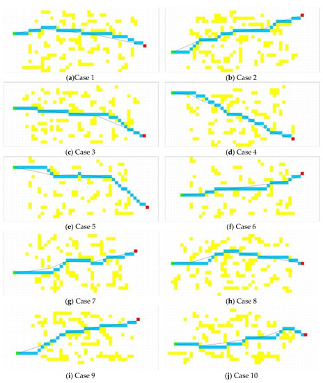
Figure 2.
Path planning for random obstacle maps.
A distinct terrain map was built to meet the requirements of a particular environment, such as an office, a gate, a narrow corridor, and spiral corridors. The experimental results are shown in Figure 3.
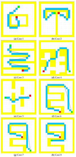
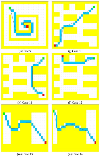
Figure 3.
Path planning in distinct maps.
4.1.2. Experimental Result Analysis
An output table can be created from the path planning results for the random obstacles map in Figure 2, as presented in Table 1.

Table 1.
Data for path planning on random obstacles maps.
Table 1 contains 10 sets of results for the algorithm planning times for the random obstacles map, shortest path length from the corresponding starting point and target point of each map, path length of the algorithm of this study, and path length for the A* algorithm.
To evaluate the degree of the planning path approach to reach the shortest path, we define the path optimal degree as follows:
where is the path length and is the length of the shortest path. When planning for the shortest path the value is 100, which is close to the planning for the optimal path. The larger the value, the closer it is to the shortest path and the planning results are better. The range of is . From Equation (26), the path optimal degrees of the algorithm proposed herein and the A* algorithm can be calculated by the random obstacles map, as shown in Table 1. The path length comparison diagram can be obtained from the data for the path planning length on the random map from Table 1, as shown in Figure 4. Additionally, from the data for the path optimal degree in this table, the path optimal degree diagram is as shown in Figure 5.
Figure 4.
Comparison of path length between A* and HEPSO on random obstacles maps.
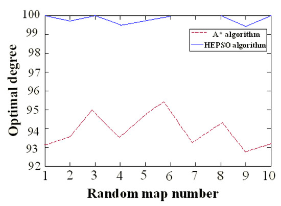
Figure 5.
Comparison of optimal degrees of A* and HEPSO algorithms on random obstacles maps.
As shown in Figure 4 and Figure 5, in the random obstacles map, the average path optimal degree of the proposed algorithm herein is 99.9% and the minimum path optimal degree is as high as 99.4%, which reaches the optimal path level. Furthermore, the range of the path optimal degree is only 0.6%. The planning results are stable. However, the average path optimal degree of the A* algorithm is 93.8%, which differs significantly from that of the optimal path. The range of the path optimal degree is 2.5% and the planning results are not stable.
The experimental results of this group of path planning on the random obstacles map shows that, for long distances, multiple obstacles, and random complex terrains, the algorithm proposed herein combines the global heuristic information and local elastic iterative strategy, rendering an average error rate of only 0.1% for the planning of the shortest path. Furthermore, because of planning the optimal path, the planning result is stable. When the average path length is 852 pixels, the average planning time is 0.2 s, thus demonstrating that the algorithm has a better real-time performance.
An output table can be constructed, from the path planning results on the distinct terrain map shown in Figure 3, as shown in Table 2. The table contains 10 sets of results, which include the algorithm planning time on the distinct terrain map, the shortest path length from the corresponding starting point, the target point of each map, the path length of the algorithm proposed herein, and the path length of the A* algorithm. From Equation (26), the path optimal degrees of the algorithm proposed herein and A* algorithm can be calculated from the random obstacles map, as presented in Table 2.
Table 2.
Data of path planning on distinct maps.
A path length comparison diagram can be constructed from the results for the path planning length using the distinct terrain map listed in Table 2, as shown in Figure 6. Using the data for the path optimal degree in Table 2, the path optimal degree diagram is as shown in Figure 7.
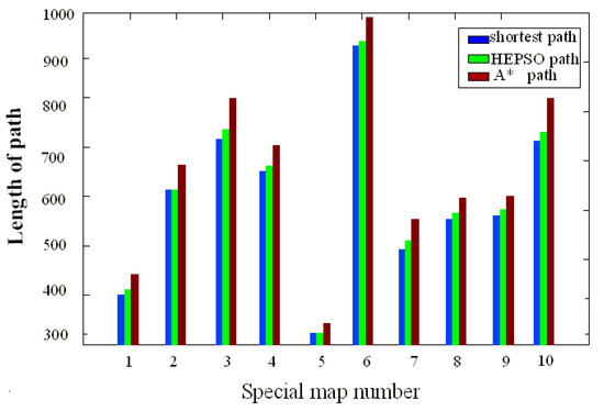
Figure 6.
Comparison of path lengths on distinct maps of A* and HEPSO algorithms.
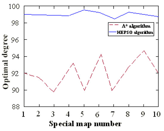
Figure 7.
Comparison of optimal degrees on distinct maps of A* and HEPSO algorithms.
As shown in Figure 6 and Figure 7 in the random obstacle map, the average path optimal degree of the algorithm proposed herein is 99.1%, which reaches the optimal path level. Additionally, the range of the path optimal degree is only 1.1%. The planning results are stable. Comparatively, the average path optimal degree of the A* algorithm is 92.2%, which differs significantly from the optimal path. Furthermore, the range of the path optimal degree is up to 5.7%. Thus, the planning results are highly unstable.
The experimental results of this group of path planning on the distinct terrain map indicate that for various unique terrains, including a narrow gate, a T shape, a zigzag, a bow, a spiral, and a tunnel shape (established according to the actual scene and practical problems), the algorithm proposed herein, by combining the global heuristic information and a local elastic iterative strategy, renders an average path length of 604 pixels and average planning time of 0.1 s, which are better real-time performances. Furthermore, the planning path with the shortest path average error rate is only 0.9%, and the shortest path is planned.
To summarize, this algorithm can ensure real-time performance, yield the shortest path, and provide stable planning results regardless of the complexity of the random obstacles map or the various structures on the distinct terrain map. Therefore, this demonstrates the efficiency and reliability of the algorithm proposed herein.
4.2. Robot Experiment
To verify the effectiveness of the path planning algorithm, we physically verified the MT-R research intelligent robot platform. The diameter of the MT-R robot was 50 cm, the maximum speed was 2.5 m/s, and the turning radius was zero.
In this study, the planning path is converted to an instruction set and the control instructions of the set are sent individually to the robot driver so that it can autonomously control the robot. The flat indoor experimental environment is comprised of two static obstacles, the starting point S(x) and target point T(x), as shown in Figure 8. The robot operation results are shown in Figure 9.
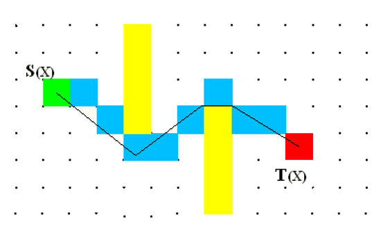
Figure 8.
Result of path planning on robot.
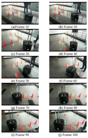
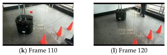
Figure 9.
Result of robot experience.
In the early stages of the research, to solve the problems of the standard robot path planning algorithm (being prone to the local minimum value problem and having a low quality), study [16] proposes an improved path planning problem. The path planning, PSO–TVAPF, was based on the tangent vector method and a particle swarm algorithm. The algorithm proposed by study [16] effectively avoids the local minimum value problem and shortens the path length. Similar experiments with real machines were performed. The heuristic PSO optimal path planning algorithm presented in this paper has achieved better real-time execution. Based on the insight gained from the efficient A* algorithm for particle initialization, to enhance its real-time properties, the algorithm uses the improved elastic PSO algorithm to iterate the initial heuristic path and performs contraction and rebound operations to avoid the local minimum problem and shorten the path length. Similar experiments are conducted. Therefore, the robot path planning by the algorithm proposed in this study shows better real-time performance then the algorithm in study [16]. However, when the classical APF encounters obstacles in the path planning, the path planning fails.
5. Conclusions
In this paper, a heuristic elastic PSO optimal path planning algorithm is proposed in which the efficient A* algorithm is used to collect heuristic information for particle initialisation. Using an improved elastic PSO algorithm, the initial heuristic path is iterated, and the particle is assembled along the optimal path using the shrink operation in the elastic strategy. Particle degradation occurs when the particles shrank to the rebound threshold. This phenomenon is overcome by a rebound operation, thus avoiding the local extremum among the particles. The simulation and robot experiment demonstrates that the algorithm herein could plan the shortest path efficiently and it achieves good performance in solving the two major problems of path planning in real time and low stability. Path planning could be optimized further for the safe and smooth operation of a mobile robot, according to its motion characteristics.
Author Contributions
Formal analysis, Z.Z.; Software, H.W.
Funding
This research received no external funding.
Conflicts of Interest
The authors declare no conflict of interest.
References
- Wu, J.; Wang, J.; You, Z. An overview of dynamic parameter identification of robots. Robot. Comput. Integr. Manuf. 2010, 26, 414–419. [Google Scholar] [CrossRef]
- Zhong, C.L.; Liu, S.R.; Lu, Q.; Zhang, B.; Yang, S.X. An efficient fine-to-coarse way finding strategy for robot navigation in regionalized environments. IEEE Trans. Cybern. 2016, 46, 3157–3170. [Google Scholar] [PubMed]
- Zhu, H.; Deng, L. A landmark-based navigation method for autonomous aircraft. Optik 2016, 127, 3572–3575. [Google Scholar] [CrossRef]
- Wu, J.; Wang, D.; Wang, L. A control strategy of a two degrees-of-freedom heavy duty parallel manipulator. J. Dyn. Syst. Meas. Control 2015, 137. [Google Scholar] [CrossRef]
- He, B.; Wang, B.; Yan, T.; Han, Y. A distributed parallel motion control for the multi-thruster autonomous underwater vehicle. Mech. Des. Struct. Mach. 2013, 42, 236–257. [Google Scholar] [CrossRef]
- Fang, Y.W.; Qiao, D.D.; Zhang, L.; Yang, P.F.; Peng, W.S. A new cruise missile path tracking method based on second-order smoothing. Optik 2016, 127, 4948–4953. [Google Scholar]
- Wu, J.; Wang, J.; Wang, L.; Li, T. Dynamics and control of a planar 3-DOF parallel manipulator with actuation redundancy. Mech. Mach. Theory 2009, 44, 835–849. [Google Scholar] [CrossRef]
- Persson, S.M.; Sharf, I. Sampling-based A* algorithm for robot path-planning. Int. J. Robot. Res. 2014, 33, 1683–1708. [Google Scholar]
- Jaillet, L.; Siméon, T. Path deformation roadmaps: Compact graphs with useful cycles for motion planning. Int. J. Robot. Res. 2008, 27, 1175–1188. [Google Scholar] [CrossRef]
- Cai, C.; Ferrari, S. Information-driven sensor path planning by approximate cell decomposition. IEEE Trans Syst. Man Cybern. B 2009, 39, 672–689. [Google Scholar]
- Ghatee, M.; Mohades, A. Motion planning in order to optimize the length and clearance applying a Hopfield neural network. Expert Syst. Appl. 2009, 36, 4688–4695. [Google Scholar]
- Du, X.; Chen, H.; Gu, W. Neural network and genetic algorithm based global path planning in a static environment. J. Zhejiang Univ. Sci. A 2005, 6, 549–554. [Google Scholar]
- Liu, J.; Yang, J.; Liu, H.; Tian, X.; Gao, M. An improved ant colony algorithm for robot path planning. Soft Comput. 2017, 21, 5829–5839. [Google Scholar]
- Mac, T.T.; Copot, C.; Tran, D.T.; De Keyser, R. A hierarchical global path planning approach for mobile robots based on multi-objective particle swarm optimization. Appl. Soft Comput. 2017, 59, 68–76. [Google Scholar]
- He, B.; Ying, L.; Zhang, S.; Feng, X.; Yan, T.; Nian, R.; Shen, Y. Autonomous navigation based on unscented-FastSLAM using particle swarm optimization for autonomous underwater vehicles. Measurement 2015, 71, 89–101. [Google Scholar]
- Zhou, Z.; Wang, J.; Zhu, Z.; Yang, D.; Wu, J. Tangent navigated robot path planning strategy using particle swarm optimized artificial potential field. Optik 2018, 158, 639–651. [Google Scholar]
- Contreras-Cruz, M.A.; Ayala-Ramirez, V.; Hernandez-Belmonte, U.H. Mobile robot path planning using artificial bee colony and evolutionary programming. Appl. Soft Comput. 2015, 30, 319–328. [Google Scholar] [CrossRef]
- Chang, W.L.; Zeng, D.; Chen, R.C.; Guo, S. An artificial bee colony algorithm for data collection path planning in sparse wireless sensor networks. Int. J. Mach. Learn. Cybern. 2015, 6, 375–383. [Google Scholar]
- Montiel, O.; Sepúlveda, R.; Orozco-Rosas, U. Optimal path planning generation for mobile robots using parallel evolutionary artificial potential field. J. Intell. Robot. Syst. 2015, 79, 237–257. [Google Scholar]
- Chang, Y.; Yoshio, Y. Path planning of wheeled mobile robot with simultaneous free space locating capability. Intell. Serv. Robot. 2009, 2, 9–22. [Google Scholar]
- Jonghoek, K.; Zhang, F.M.; Magnus, E. A provably complete exploration strategy by constructing Voronoi diagrams. Auton. Robots 2010, 29, 367–380. [Google Scholar]
- Xin, Y.; Liang, H.; Du, M.; Mei, T.; Wang, Z.L.; Jiang, R.H. An improved A* algorithm for searching infinite neighborhoods. Robot 2014, 36, 627–633. [Google Scholar]
- Feng, X.; Ma, M.; Shi, Y.; Yu, H. Path planning for mobile robots based on social group search algorithm. J. Comput. Res. Dev. 2013, 50, 2543–2553. [Google Scholar]
- Ao, Y.; Shi, Y.; Zhang, W.; Li, Y. Improved particle swarm optimization with adaptive inertia weight. J. Univ. Electron. Sci. Technol. China 2014, 43, 874–880. [Google Scholar]
- Jiang, J.; Tian, M.; Wang, X.; Long, X.; Li, J. Adaptive particle swarm optimization algorithm via disturbing acceleration coefficients. J. Xidain Univ. 2012, 39, 74–80. [Google Scholar]
- Gong, D.; Zhang, J.; Zhang, Y. Multi-objective particle swarm optimization for robot path planning in environment with danger sources. J. Comput. 2011, 6, 1554–1561. [Google Scholar] [CrossRef]
- Jia, H.; Wei, Z.; He, X.; Zhang, L. Path planning based on improved particle swarm optimization algorithm. Trans. Chin. Soc. for Agric. Mach. 2018, 49, 102–105. [Google Scholar]
© 2019 by the authors. Licensee MDPI, Basel, Switzerland. This article is an open access article distributed under the terms and conditions of the Creative Commons Attribution (CC BY) license (http://creativecommons.org/licenses/by/4.0/).