Hybrid LSTM Neural Network for Short-Term Traffic Flow Prediction

Abstract

The existing short-term traffic flow prediction models fail to provide precise prediction results and consider the impact of different traffic conditions on the prediction results in an actual traffic network. To solve these problems, a hybrid Long Short–Term Memory (LSTM) neural network is proposed, based on the LSTM model. Then, the structure and parameters of the hybrid LSTM neural network are optimized experimentally for different traffic conditions, and the final model is compared with the other typical models. It is found that the prediction error of the hybrid LSTM model is obviously less than those of the other models, but the running time of the hybrid LSTM model is only slightly longer than that of the LSTM model. Based on the hybrid LSTM model, the vehicle flows of each road section and intersection in the actual traffic network are further predicted. The results show that the maximum relative error between the actual and predictive vehicle flows of each road section is 1.03%, and the maximum relative error between the actual and predictive vehicle flows of each road intersection is 1.18%. Hence, the hybrid LSTM model is closer to the accuracy and real-time requirements of short-term traffic flow prediction, and suitable for different traffic conditions in the actual traffic network.

1. Introduction

With the continuous expansion of urban size, the scale of urban traffic network is growing, and the number of vehicles is also increasing. As a result, traffic congestion has gradually evolved into an unavoidable problem. It is necessary to predict the short-term traffic flow of the traffic network precisely and guide the traffic based on the prediction results, so as to enhance people’s travel experience, alleviate the traffic congestion problem, and provide a good decision support for the government to carry out the planning and construction of public traffic infrastructure.

At present, researchers have proposed many traffic flow prediction models, which are mainly divided into the following two categories. One is the type of models based on mathematical and physical methods, the other is the type of models based on simulation technology, neural network, fuzzy control, and other modern scientific and technological methods. The former mainly includes historical average method, parametric regression model, Auto Regressive Integrated Moving Average (ARIMA) model, Kalman filtering model, exponential smoothing model, etc. [1,2,3,4,5,6,7] (see Section 2). The latter mainly includes non-parametric regression model, spectral analysis method, wavelet neural network, complex prediction models combined with various intelligent algorithms, etc. [8,9,10,11,12,13,14,15,16,17,18,19,20,21] (see Section 2). In addition, there are many other prediction models, such as the Markov model, Deep Belief Network (DBN), etc. [22,23,24,25,26,27,28,29] (See Section 2). In order to obtain dependent relationship among sequence data, Boon-Hee Soong et al. [30] suggested using a Long Short–Term Memory (LSTM) model to predict traffic flow. However, the above prediction models fail to provide precise prediction results and consider the impact of different traffic conditions on the prediction results in the actual traffic network.

The aim of this paper is the development of a traffic flow prediction model, able to provide precise prediction results and suitable for different traffic conditions in the actual traffic network. Based on the LSTM model, we present a hybrid LSTM neural network, and experimentally optimize its structure and parameters for different traffic conditions. And we further apply the hybrid LSTM model to the vehicle flow prediction of each road section and intersection in the actual traffic network. The experimental results indicate that our proposed hybrid LSTM model provides more accurate prediction results than the other typical models, and suitable for different traffic conditions in the actual traffic network.

The remainder of this article is organized as follows. Section 2 provides an overview of the existing solutions for traffic flow prediction models. In Section 3, we provide the rationale of our proposed hybrid LSTM neural network. Section 4 describes in detail the experimental process. In Section 5, we present the experimental results, and concludes the paper in Section 6.

2. Related Works

In terms of prediction models based on mathematical and physical methods, Okutani et al. [1] proposed two models employing Kalman filtering theory for predicting short-term traffic flow. In the two models, prediction parameters are improved using the most recent prediction error and better volume prediction on a link, which is achieved by taking into account data from a number of links. Perera et al. [2] proposed an extended Kalman filter as an adaptive filter algorithm for the estimation of position, velocity and acceleration that are used for prediction of maneuvering ocean vessel trajectory. Chen et al. [3] proposed an Autoregressive Integrated Moving Average with Generalized Autoregressive Conditional Heteroscedasticity (ARIMA-GARCH) model for traffic flow prediction. The model combines linear ARIMA with nonlinear GARCH, so it can capture both the conditional mean and conditional heteroscedasticity of traffic flow series. Shen et al. [4] proposed a combination prediction model including Kalman filter and radial basis function neural network, and introduced inertia factor to ensure the stability of the hybrid model. Zhu et al. [5] put forward a model that combines Kalman filter with Support Vector Machine (SVM). The model adopts appropriate forecast method intelligently in each prediction period by the maximum standards of error sum of squares and vector cosine of the angle, utilizes the stability of SVM and the real-time nature of Kalman filter, and takes respective advantages of the two models. Yang et al. [6] combined ARIMA model with Kalman filter through the error magnitude of predictive results to predict the traffic flow in a road. Tang et al. [7] developed a hybrid model that combines Double Exponential Smoothing (DES) and SVM to implement a traffic flow predictor. In the hybrid model, DES is used firstly to predict the future data, and the smoothing parameters of DES are determined by Levenberg-Marquardt algorithm.

In terms of prediction models based on modern scientific and technological methods such as simulation technology, neural network and fuzzy control, Li et al. [8] proposed a prediction method of optimized Back Propagation (BP) neural network based on a modified Particle Swarm Optimization (PSO) algorithm. By introducing adaptive mutation operator to change positions of the particles with plunged in the local optimum, the modified PSO was used to optimize the weight and thresholds of BP neural network, and then the optimized BP neural network was trained to search for the optimal solution. Liu [9] proposed a model based on the combination of phase reconstruction and Support Vector Regression (SVR). The parameters of phase reconstruction and SVR are optimized by PSO in this model. Gao [10] proposed a model based on cuckoo search algorithm and BP neural network. The time series of short-term traffic flow is reconstructed to form a multidimensional time series based on chaotic theory, and then the time series are input into BP neural network to find the optimal parameters of BP neural network based on the cuckoo search algorithm. Zhang et al. [11] introduced boundary mutation operator and self-adaptive mutation operator called double mutation to optimize network configuration parameters based on the traditional BP neural network optimized by PSO. Hou et al. [12] proposed a prediction algorithm for traffic flow of T-S Fuzzy Neural Network optimized Improved Particle Swarm Optimization (IPSOTSFNN) to make the algorithm to jump out of local optimum by using t distribution. Shen et al. [13] presented a model which is based on the wavelet neural network optimized by Chaos Particle Swarm Optimization (CPSO). In combination of the randomness and ergodicity of chaos, the particle swarm optimization algorithm is improved to avoid falling into local optimum. Based on K-means clustering, Zang et al. [14] integrated Elman Neural Network (Elman-NN) with wavelet decomposition method to characterize the performance comparison of traffic flow prediction. Minal et al. [15] suggested the application of a neural-fuzzy hybrid method which brought together the complementary capabilities of both neural networks and fuzzy logic, and involved the combination of the least square estimation and back propagation. Kumar [16] used an artificial neural network model with multiple input parameters and developed a variety of models according to different combinations of input parameters. Yu et al. [17] used the principal component analysis algorithm to reduce the dimensions of data, and discussed the establishment and improvement of BP neural network according to the problem of input nodes, initial connection weights and excitation functions. Zhang et al. [18] established an Elitist Adaptive Genetic Algorithm (EAGA) by combining Elitist Adaptive Genetic Algorithm (EGA) with Adaptive Genetic Algorithm (AGA), and then used the EAGA to optimize BP neural network. Zhang et al. [19] presented a method based on GA-Elman neural network. In this method, the weights and threshold values of the Elman neural network are optimized by genetic algorithm, so the defect that Elman neural network is susceptible to falling into local optimum is overcome. Yi et al. [20] suggested a deep learning neural network based on TensorFlow for real-time traffic flow prediction. Yin et al. [21] analyzed the relationship between the embedding dimension of phase space reconstruction of traffic flow chaotic time series and Volterra discrete model, and proposed a method to determine the truncation order and items of Volterra series. Then, a Volterra neural network traffic flow (VNNTF) time series model was further proposed, and multi-step prediction experiments based on Volterra prediction filter and BP network were performed.

In terms of other prediction models, Emilian [22] used a hybrid approach based on variable-order Markov model to predict traffic flow, and added the average speed of all vehicles passing through each road section. Surya et al. [23] suggested predicting traffic congestion based on real-time traffic data of each section, and controlling traffic lights at road intersections. According to the optimal action selection strategy combined with Markov Decision Process (MDP), the optimal duration of each traffic light was obtained by calculating the congestion factor at each signal change. Luo et al. [24] proposed a prediction model which combined DBN with SVR classifier. The prediction model used DBN model to extract traffic flow characteristics, and then carried traffic flow prediction with SVR in the top level of the DBN. Zhang [25] used the flaw data collected by the detectors embedded at the road intersections to obtain clustering patterns based on Fuzzy C-Means (FCM) clustering analysis, and used the traffic flow at the road intersection of the same pattern to predict the traffic flow at another road intersection. Rui et al. [26] proposed an algorithm which combined a flow sequence partition and Extreme Learning Machine (ELM). The algorithm divided the traffic flow into different patterns along a time dimension by K-means, and then modelled and predicted for each pattern by ELM. Pascale et al. [27] investigated a statistical method based on the graphical modeling of traffic spatial-temporal evolution, and then proposed an adaptive Bayesian network where the network topology is changed following by the non-stationary characteristics of traffic. Wen et al. [28] suggested an adaptive particle filter algorithm based on confidence interval, which can adaptively adjust the number of particles according to the state of particles and reduce the quantity of the particle filter algorithm calculation so as to improve the real time capability. Borkowski [29] proposed a ship motion trajectory prediction algorithm, which effectively solves the collision problem by data fusion and taking into account measurements of the ship’s current position from a number of doubled autonomous devices. Shao et al. [30] used a LSTM model to predict short-term traffic flow, where the dependency relationships of series data are fully considered, but the final experimental results show that the Root Mean Square Error (RMSE) value of prediction is 40.34.

3. Hybrid LSTM Neural Network

Neural networks show great advantages in prediction because of its unique non-linear adaptive processing ability. Generally, the short-term traffic flow prediction should be based on the previous several time steps and dependencies between the time series, which is impossible to be finished by traditional neural networks. Using previous events to infer subsequent events is usually to be done with Recurrent Neural Network (RNN) [31].

In the process of training neural networks, gradient descent method is usually used to evaluate the network performance. But in the traditional RNN, the training algorithm is the Back Propagation Through Time (BPTT). Consequently, if the training time is long, then the residual of the network needing to be returned will decrease exponentially, leading to the slow renewal of network weights. That is to say, the traditional RNN appear vanishing gradient problem, which cannot reflect the effect of long-term memory in practical applications, so a memory block is needed to store memory. Therefore, a special RNN model was proposed, namely LSTM model [32], which can preserve long-term dependencies and read any length sequence. And there is no relationship between the number of neurons and the length of sequences in the LSTM model. However, it can be seen that the LSTM model meets the real-time requirement of traffic flow prediction, but does not meet the accuracy requirement of traffic flow prediction [30]. Therefore, we propose a hybrid LSTM neural network based on the LSTM model in the paper, and optimize the network structure and parameters of the hybrid LSTM experimentally for different traffic conditions, so that the hybrid LSTM model can satisfy the above two requirements of traffic flow prediction at the same time.

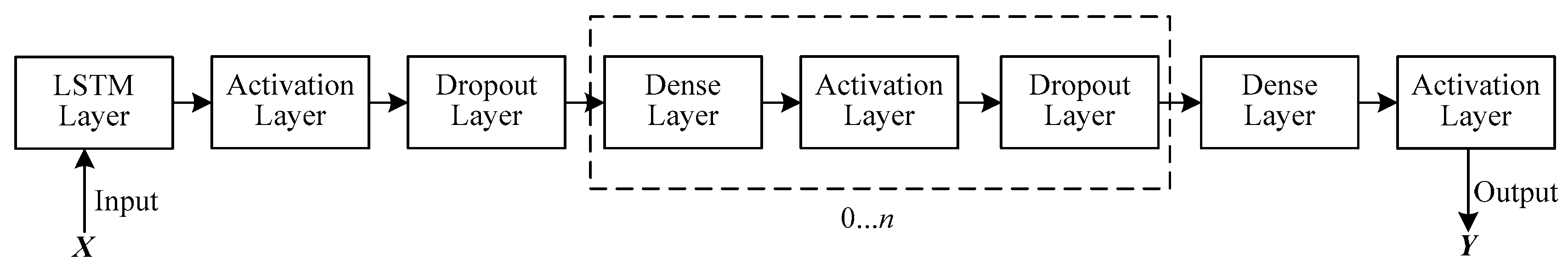
3.1. Network Structure

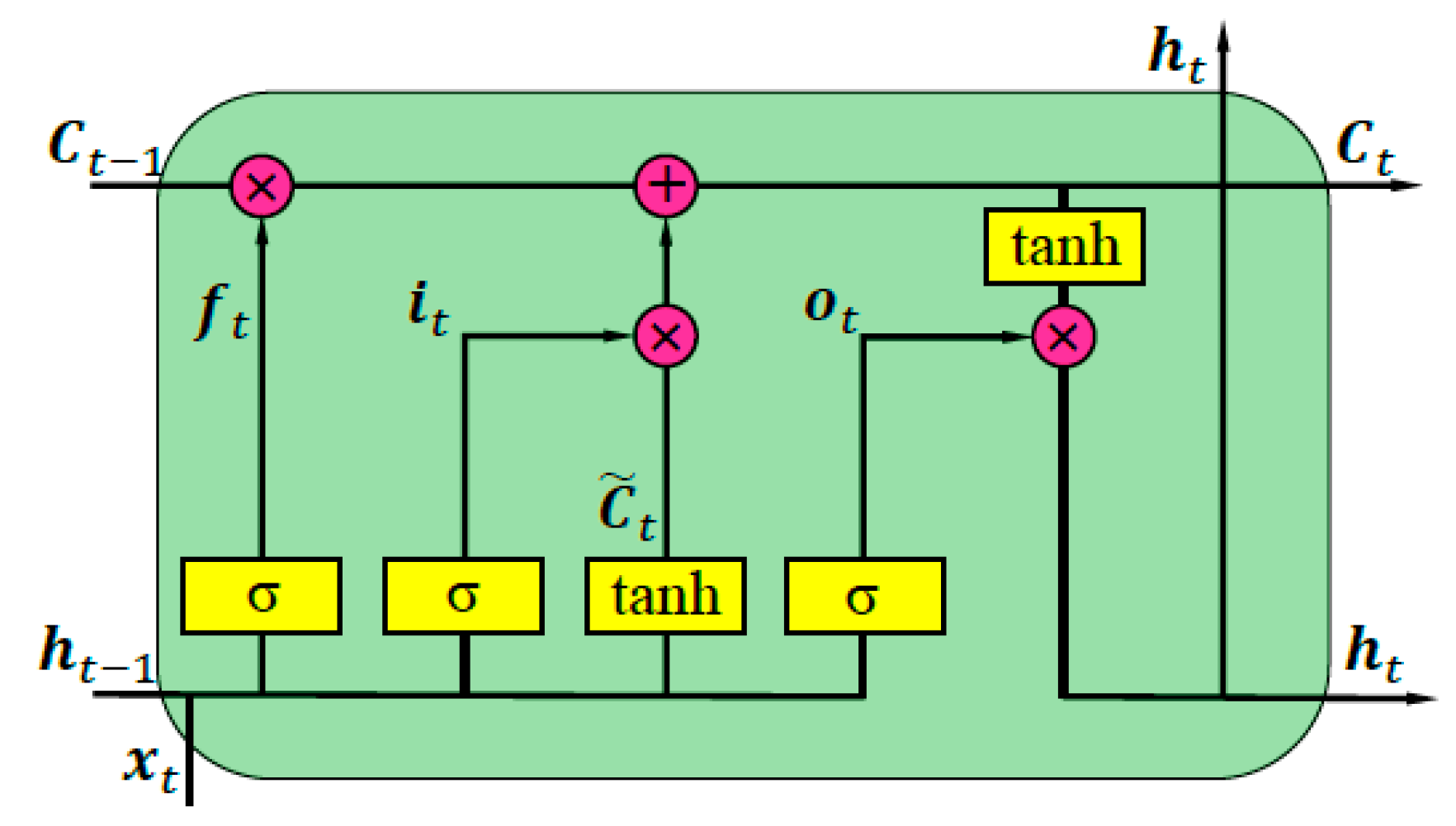
To improve the accuracy of short-term traffic flow prediction, a hybrid LSTM neural network structure is proposed in this paper, as shown in Figure 1.

Figure 1. Hybrid Long Short–Term Memory (LSTM) neural network structure.

In Figure 1, the hybrid LSTM neural network structure consists of one input combination layer, zero or more intermediate combination layers and one output combination layer. The input combination layer includes a LSTM layer, an Activation layer and a Dropout layer. The intermediate combination layer includes a Dense layer, an Activation layer and a Dropout layer. And the output combination layer includes a Dense layer and an Activation layer. The input of the LSTM layer of the input combination layer is X, while the output of the Activation layer of the output combination layer is Y. The Dropout layer means that some neural units are temporarily discarded from the neural network according to a certain probability during the training process, preventing over-fitting.

3.2. LSTM Layer

The LSTM layer consists of a series of LSTM units, called LSTM model [32]. Compared with other neural networks, the LSTM model has three multiplicative units, i.e., input gate, output gate and forget gate. The input gate is used to memorize some information of the present, the output gate is used for output, and the forget gate is used to choose to forget some information of the past. The multiplicative unit is mainly composed of a sigmoid function and a dot product operation, where the sigmoid function has a range of [0, 1] and the dot product operation can determine how much information is transmitted. If the value of the dot product operation is 0, then no information is transmitted. And all information is transmitted if the value of the dot product operation is 1. The LSTM unit [32] is shown in Figure 2.

Figure 2. LSTM unit.

In Figure 2, $f_t$ denotes the forget gate, $i_t$ denotes the input gate, and $o_t$ denotes the output gate, which together control the cellular state $C_t$ that stores historical and future information. $x_t$ and $h_t$ respectively represent input and output information of the LSTM unit. The processing expressions of the LSTM unit [32] are as follows:

$$f_t=\sigma (W_f\cdot [h_{t-1},x_t]+b_f)$$

(1)

$$i_t=\sigma (W_i\cdot [h_{t-1},{\mathit{x}}_t]+b_i)$$

(2)

$${\tilde{C}}_t=\tanh (W_C\cdot [h_{t-1},x_t]+b_C)$$

(3)

$$C_t=f_t\ast C_{t-1}+i_t\ast {\tilde{C}}_t$$

(4)

$$o_t=\sigma (W_o[h_{t-1},x_t]+b_o)$$

(5)

$$h_t=o_t\ast \tanh (C_t)$$

(6)

Equation (1) is a forget gate expression, which takes the weighted sum of the state of the cell at time t, the output of cell at time t − 1, and the input at time t as the input of activation function to get the output of the forget gate. The activation function is generally a logistic sigmoid function. Equation (2) is an input gate expression, where the parameters and principles are the same as those of Equation (1). Equation (3) calculates the candidate value of memory unit at the time t, where the activation function can be a tanh function or a logistic sigmoid function. Equation (4) combines past and present memories. Equation (5) is an output gate expression, where the parameters and principles are identical with those of Equation (1). Equation (6) is an expression for cell output, where the activation function is generally a tanh function. W is a weight vector matrix, and b is a bias vector.

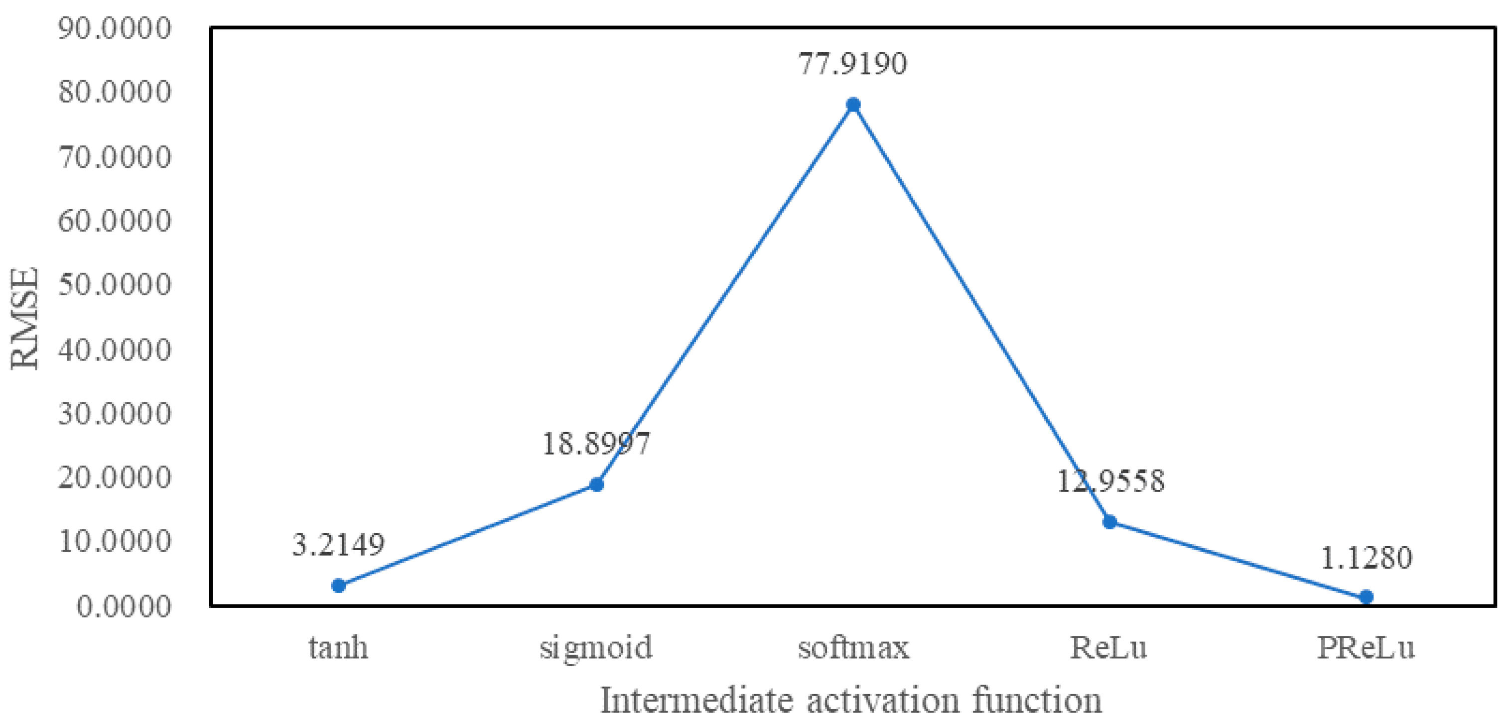
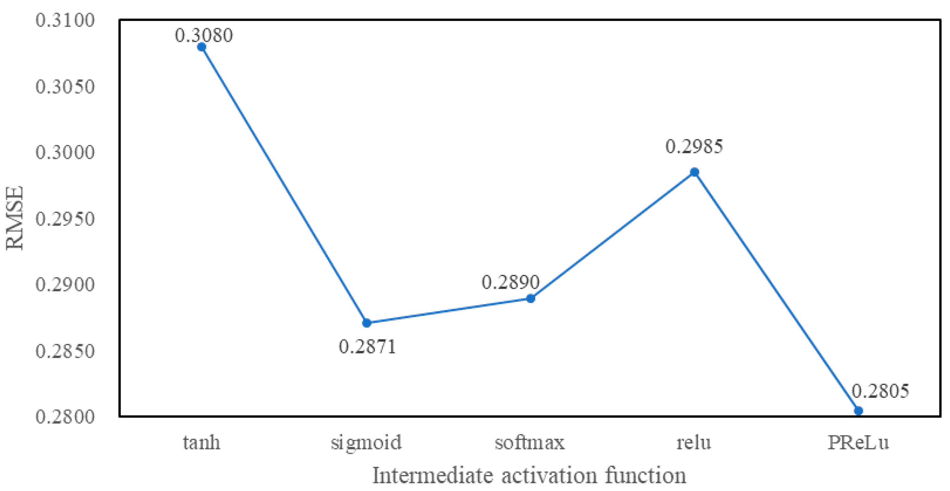
3.3. Activation Layer

The Activation layer is mainly used to improve the fitting ability of the model. In Figure 1, each combination layer contains an Activation layer. The activation layer of the output combination layer can use specific activation functions, such as logistic sigmoid function for binary classification and SoftMax function for multiple classification [33]. There are many activation functions that can be used to the Activation layers of the input and intermediate combination layers, such as tanh function, sigmoid function, Rectified Linear Unit (ReLU) function, linear function, hard-linear function, etc., and Maxout function, LeakyReLU function, Parametric Rectified Linear Unit (PReLU), softsign function, etc. [33,34,35,36], which were newly proposed in recent years.

The PReLU function is a ReLU function with parameters [34]. The mathematical expression of the PReLU function [34] is as follows.

$$\mathrm{PReLU}(x_i)=\{\begin{array}{ll}{x}_i& \mathrm{if} x_i>0\\ a_i{x}_i& \mathrm{otherwise}\end{array}$$

(7)

In Equation (7), the PReLU function becomes a ReLU function if $a_i=0$ (subscript i represents different channels). The PReLU function only adds a very small number of parameters, which means that the network’s computational complexity and the possibility of over-fitting will increase, but these changes can be neglected. In particular, the parameters are even less when different channels use the same $a_i$.

The tanh function is completely differentiable [33]. Its function image is anti-symmetric and its symmetric center is at the origin, so its output is zero center. The mathematical expression of the tanh function [33] is as follows.

$$f(x)=\frac{\sinh x}{\cosh x}=\frac{e^x-e^{-x}}{e^x+e^{-x}}$$

(8)

However, like many traditional activation functions of neural networks, the tanh function has the vanishing gradient problem. Once the value of the tanh function reaches saturation area, the gradient begins to vanish, and the learning speed becomes slower. To alleviate these problems, researchers proposed a variant of the tanh function, called softsign function [35]. The softsign function is anti-symmetric, decentralized, fully differentiable and returns values between −1 and 1. But the difference is that the slope of the softsign function is smaller than that of the tanh function in the activation area, and the softsign function enters the saturation area later than the tanh function. The mathematical expression of the softsign function [35] is as follows.

$$f(x)=\frac{x}{1+\left|x\right|}$$

(9)

The softplus function is a smooth form of the ReLu function [36], and the original function of the logical sigmoid function. The mathematical expression of the softplus function [36] is as follows.

$$f(x)=\log (1+e^x)$$

(10)

3.4. Dense Layer

The Dense layer mainly classifies feature vectors and maps the samples from the feature space to the labels [37]. It consists of two parts: the linear part and the nonlinear part. The linear part mainly performs linear transformation and analyzes the input data, the calculation method of this part is linear weighted sum, whose mathematical expression [37] is as follows:

$$Z=W\ast X+b$$

(11)

where $Z$ is the output vector of the linear part. It can be expressed as $Z={[Z_1,Z_2,\cdot \cdot \cdot ,Z_m]}^T$. $X$ represents the input vector of the linear part, which is expressed as $X={[X_1,X_2,\cdot \cdot \cdot ,X_n]}^T$. $W$ is a weight vector matrix of $m\ast n$. And $b$ is a bias vector, which is expressed as $b={[b_1,b_2,\cdot \cdot \cdot ,b_m]}^T$.

The nonlinear part performs nonlinear transformation, namely corresponding function transformation. This operation has two functions as follows. (1) Data normalization. That is to say, no matter what the previous linear part does, all the values of the nonlinear part will be limited to a certain range. (2) Break the linear mapping relation before. In other words, if the Dense layer has no non-linear part, it is meaningless to add multiple neural networks in the model.

4. Experimental Process

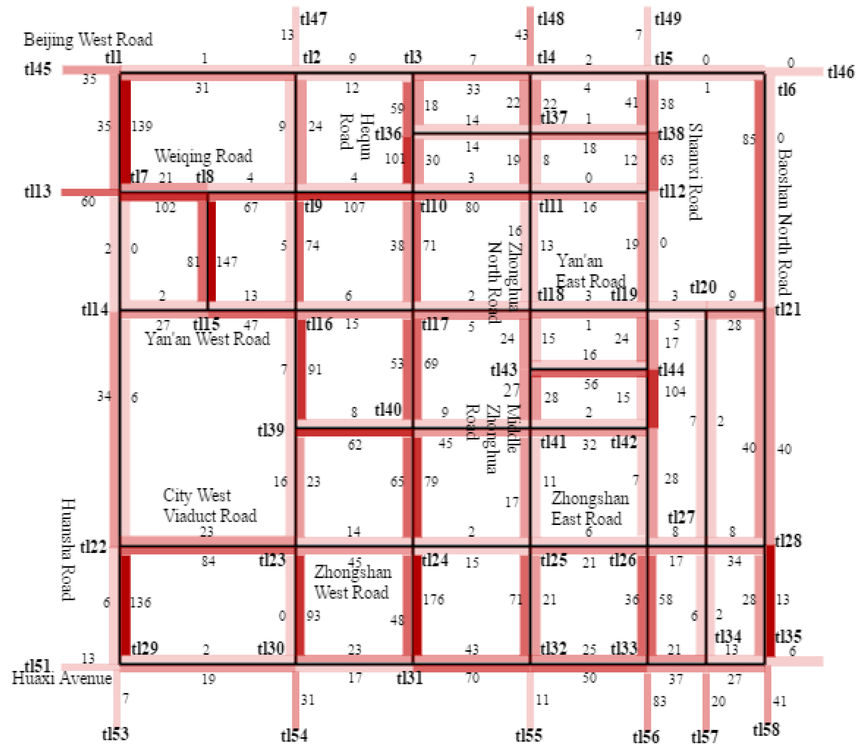
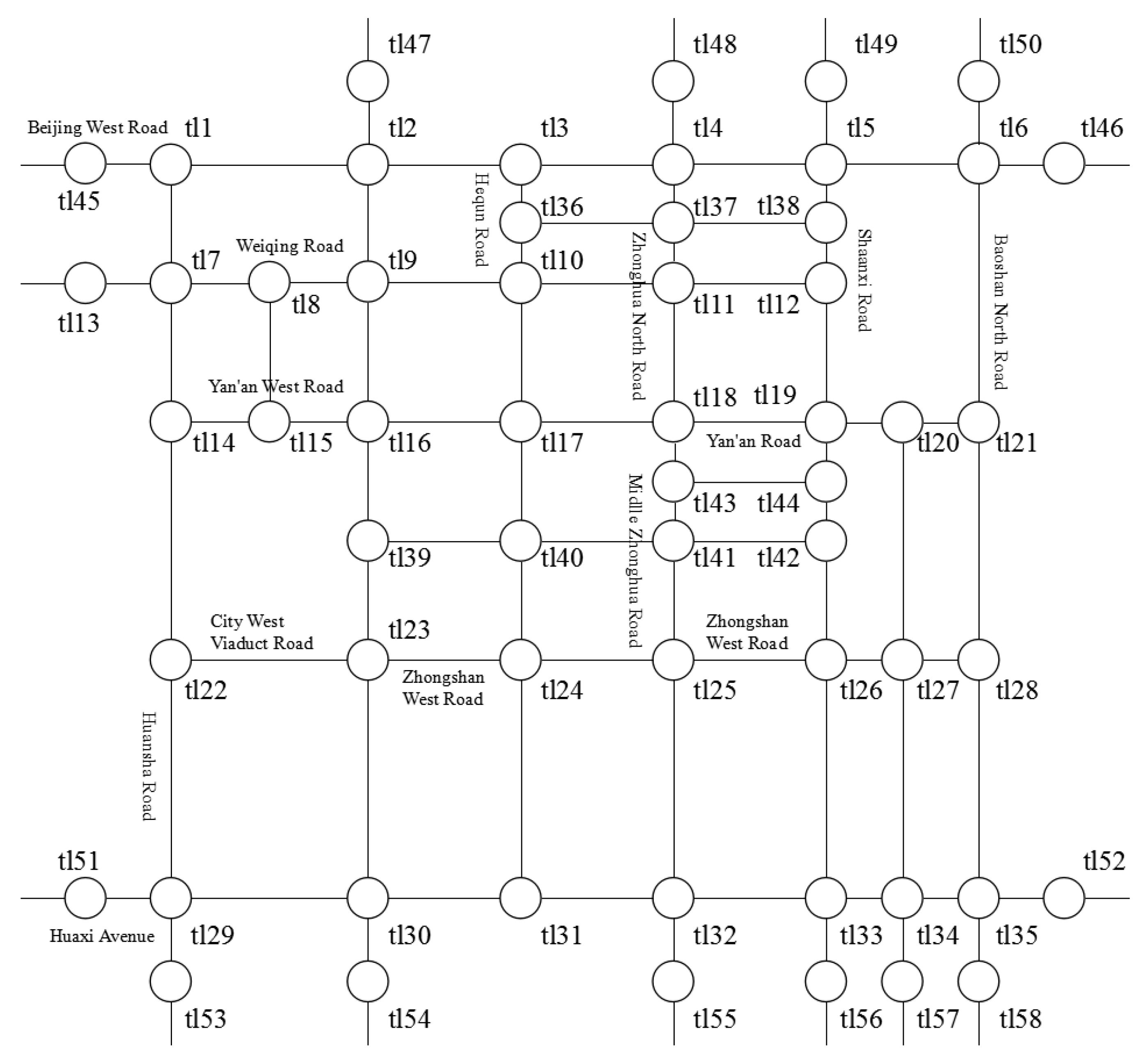
4.1. Experimental Environment and Data Set

The experimental environment in this paper is as follows: Intel (R) Core (TM) i5-3210M 2.5 GHz dual-core processor with 4 GB memory, Windows 7 64 bit operating system, the programming language is Python, and the deep learning framework is Keras. The experimental data set is the local road network traffic data from September 1st to September 8th in Yunyan District, Guiyang City, Guizhou Province. The data set contains more than 230,000 vehicle records. Each record in the original data set has three fields, which are respectively Current Node (TrafficLightID), Source Node (FromID) and Traffic Flow (traffic_flow), as shown in Table 1.

Table 1. Data fields.

Current Node (TrafficLightID)	Source Node (FromID)	Traffic Flow (traffic_flow)
tl4	tl1	[10, 8, 5, 0, 0, 23, 13, …, 23]
tl4	tl2	[23, 15, 12, 12, 9, 9, 9, …, 9]

In Table 1, TrafficLightID denotes the traffic light identifier of the vehicle currently, while FromID denotes the traffic light identifier of the vehicle at the last moment. Because the experimental data of each day is collected at a 30 s interval from 6:00 a.m. to 8:00 p.m., the traffic_flow field is a matrix of dimension 1680, which is used to represent the traffic flows of a road section at a 30 s interval. For example, traffic_flow[0] represents the traffic flow from road intersection FromID to road intersection TrafficLightID at $t_0$.

The local road network structure involved in the experimental data set is shown in Figure 3, where the hollow circles represent various intersections, the sides of the hollow circles are marked with the unique identification number of them, and the solid lines represent the road sections.

Figure 3. Local road network structure diagram.

4.2. Experimental Evaluation Indicators

Loss function is also called objective function, and the commonly used loss functions include Mean Squared Error (MSE), binary cross entropy, Mean Absolute Error (MAE), Mean Absolute Percentage Error (MAPE) [30]. In this paper, RMSE is used to evaluate the performance of the hybrid LSTM model because this method can reduce the impact of gross error on the result, and the unit of the result is the same as that of the predicted data, namely the size of the traffic flow. The mathematical expression of RMSE [30] is as follows:

$$RMSE=\sqrt{\frac{1}{n}{\displaystyle \sum _{i=1}^n{w}_i}{(y_i-{\widehat{y}}_i)}^2}$$

(12)

where $n$ is the number of samples, $y_i$ is the true value of samples, and ${\widehat{y}}_i$ is the corresponding predictive value.

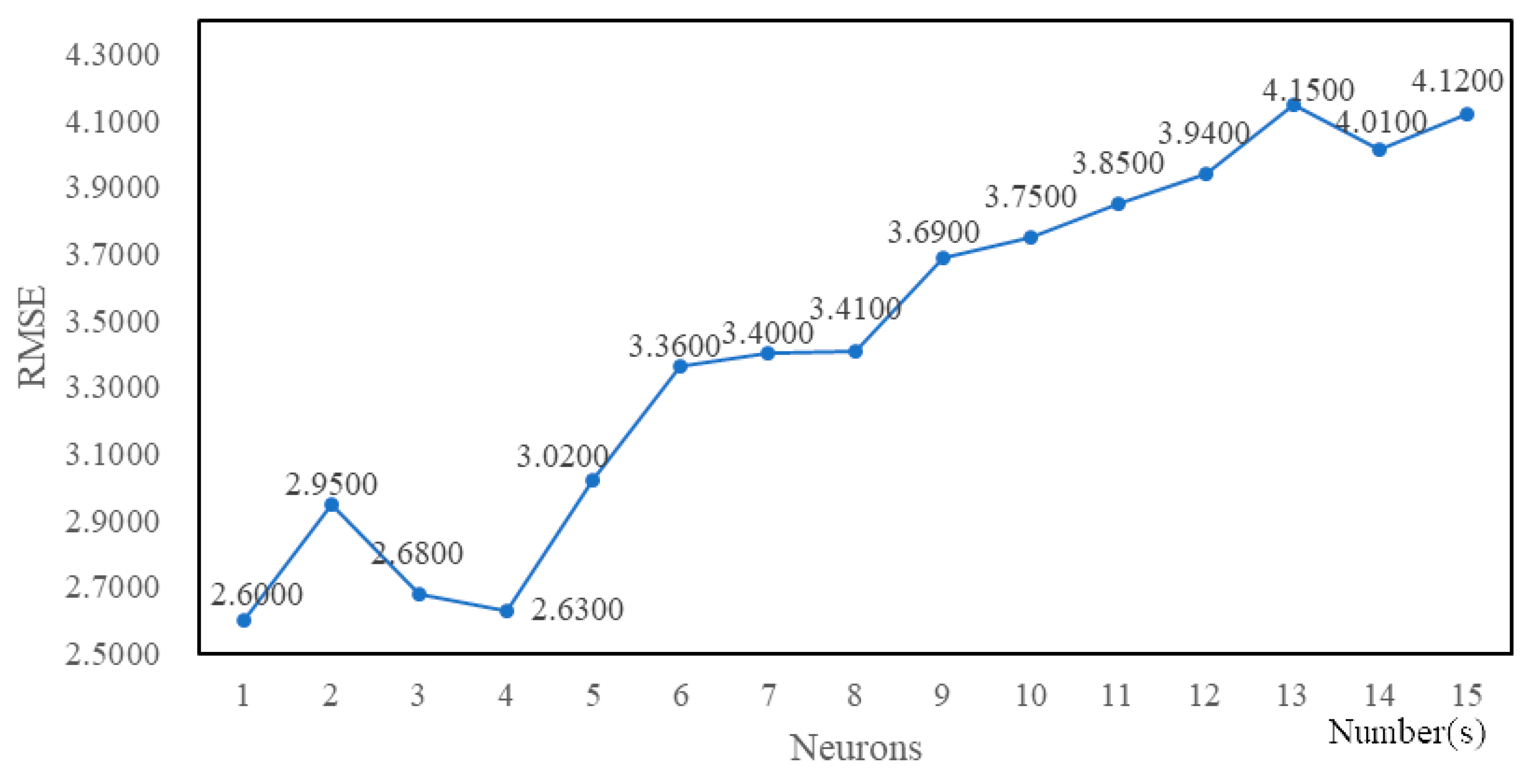
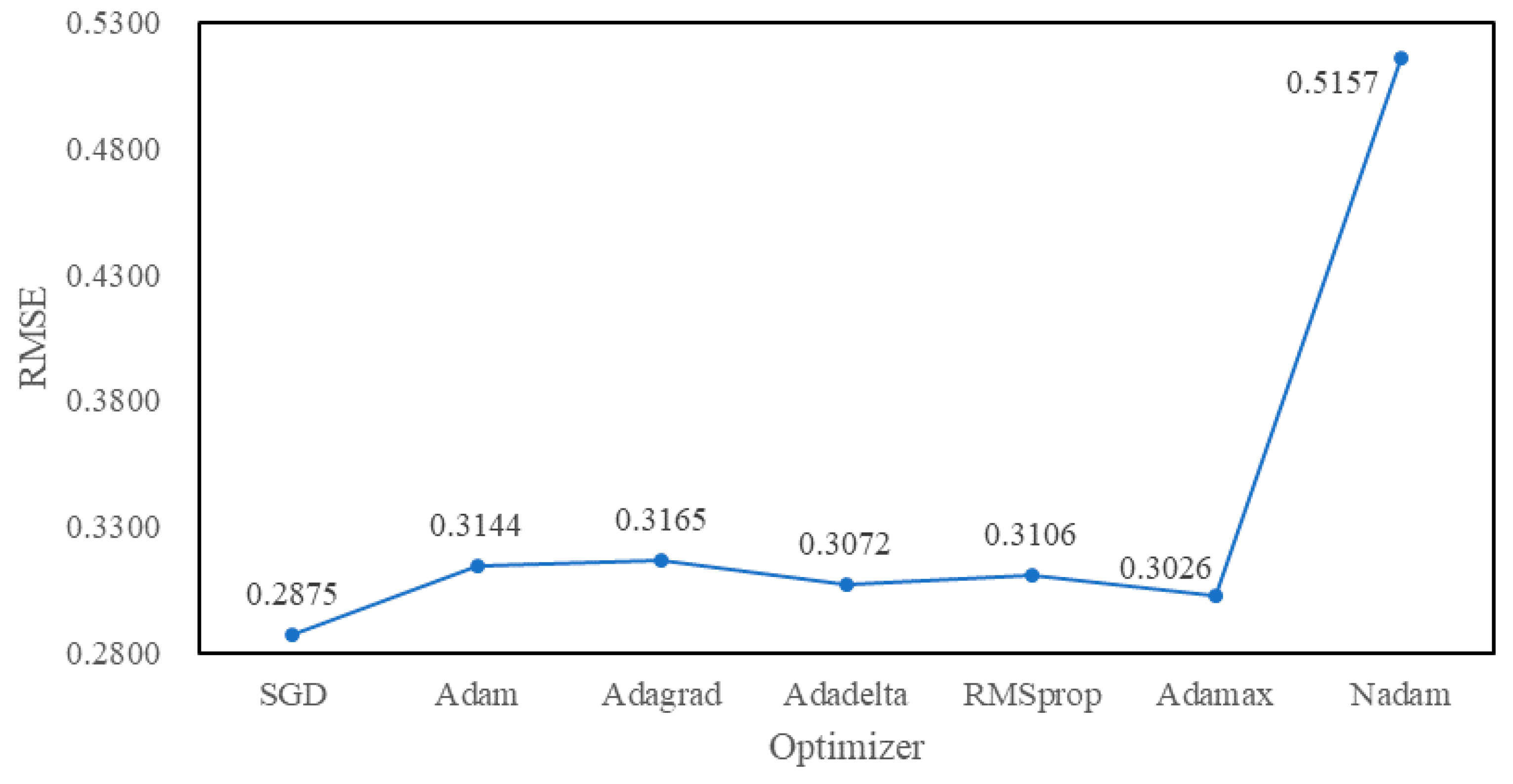
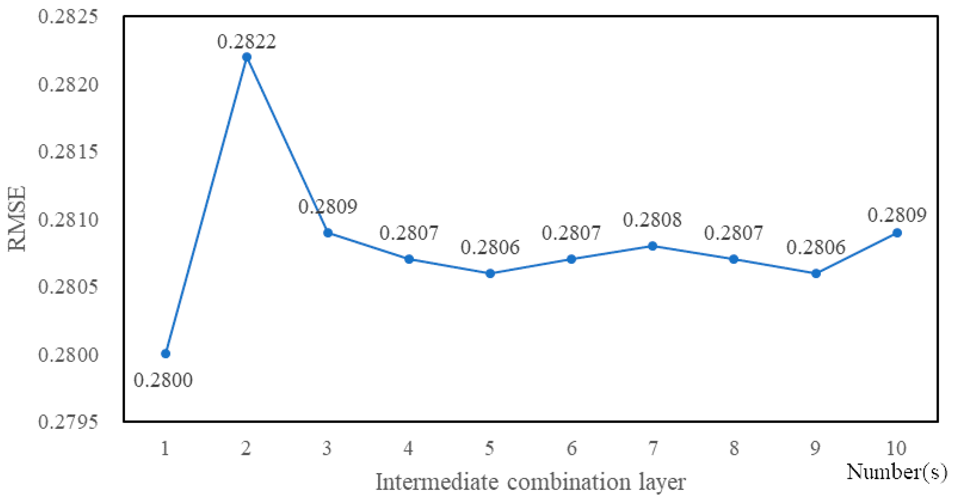
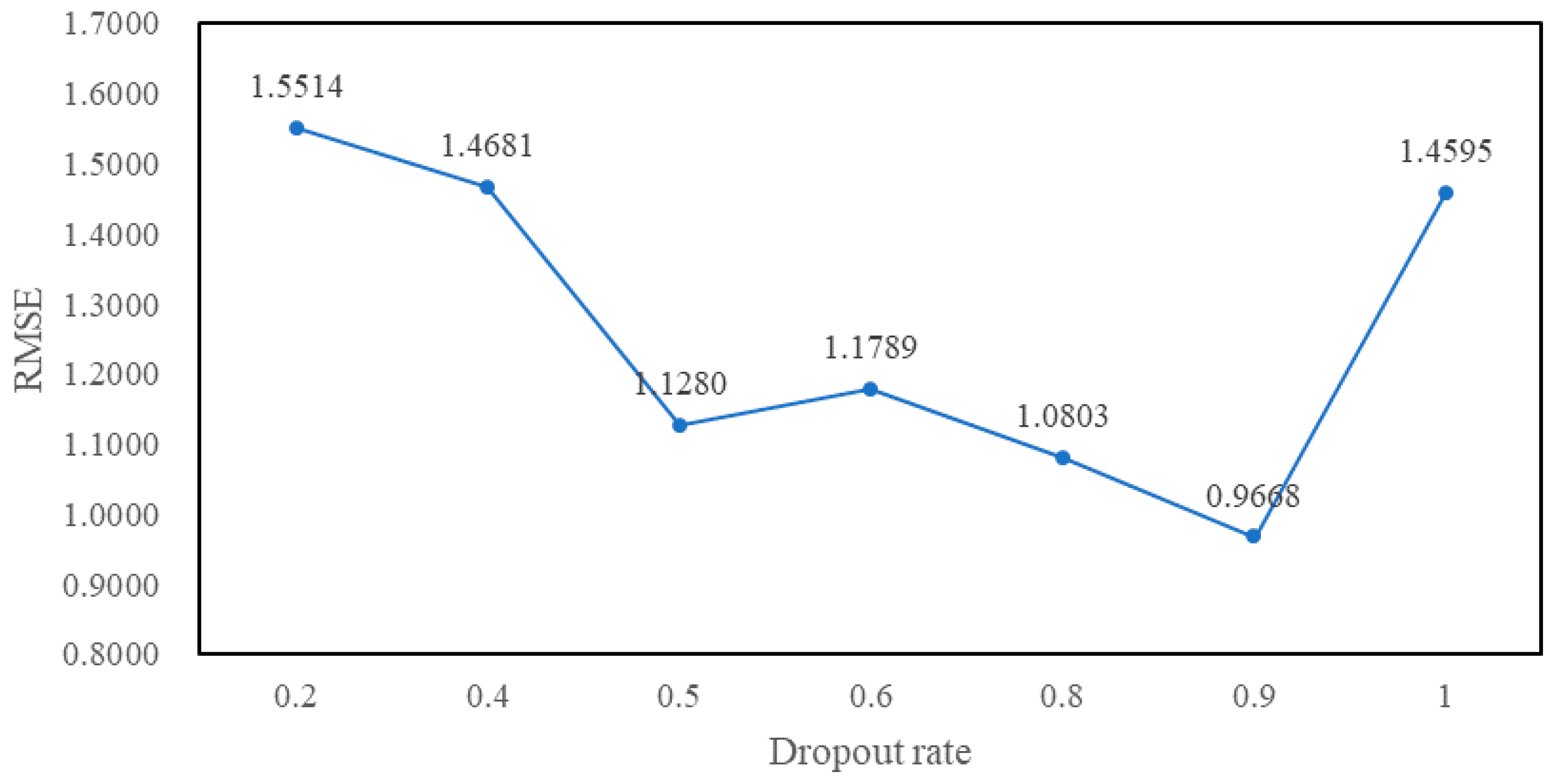
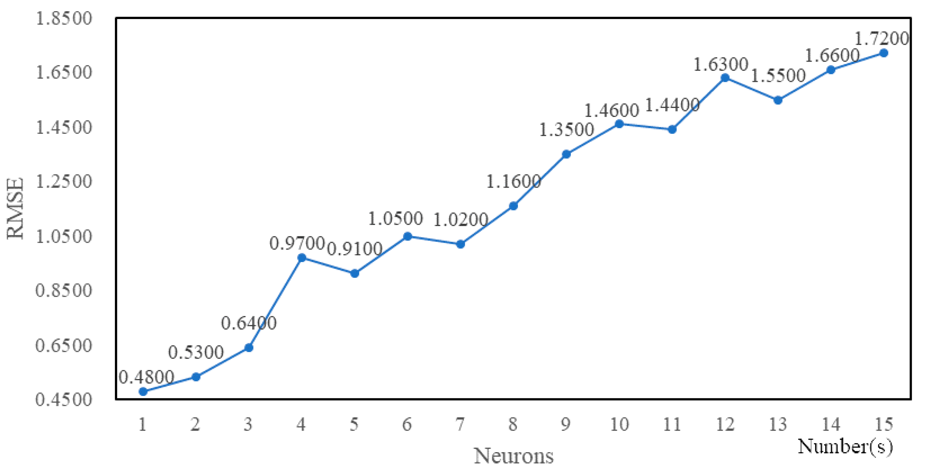
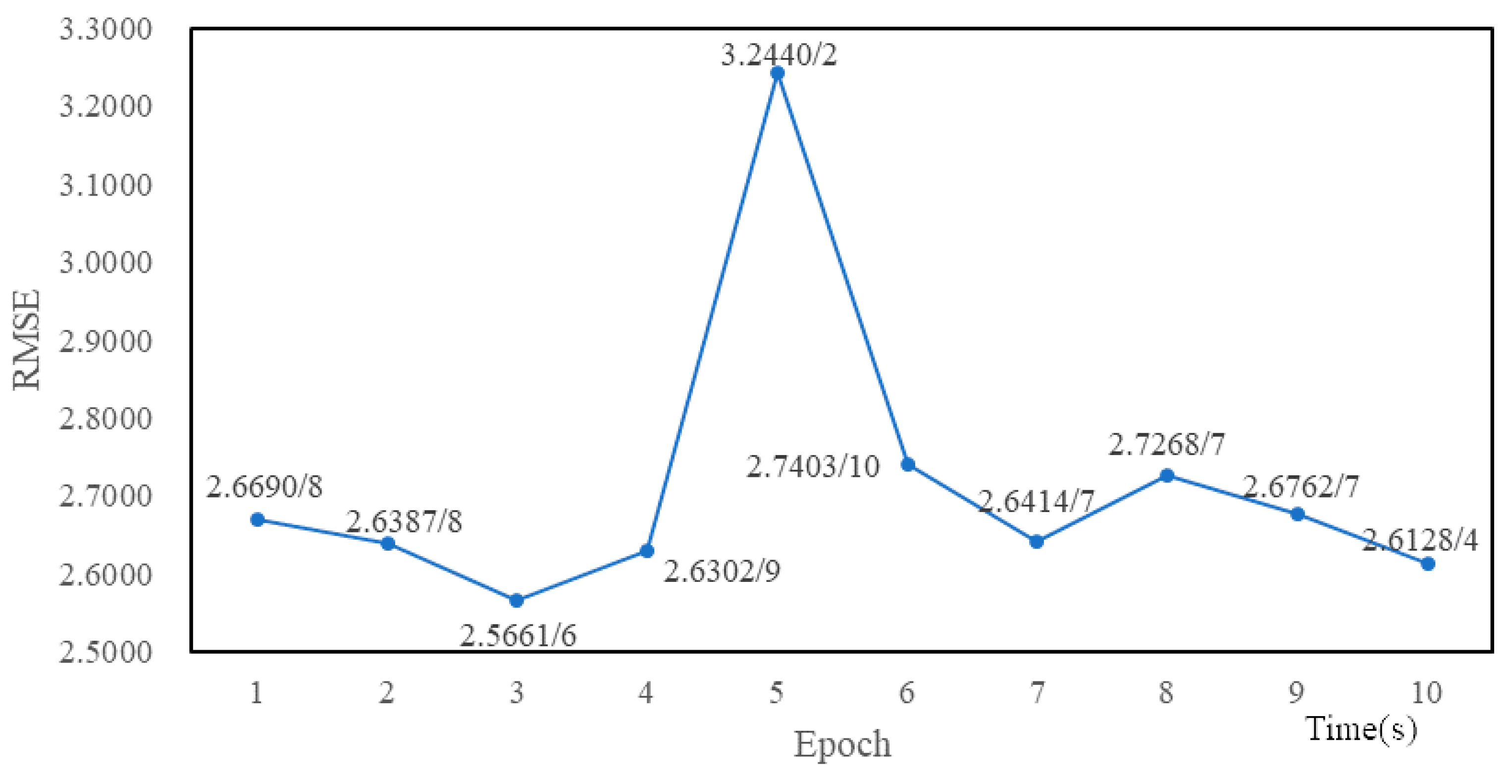
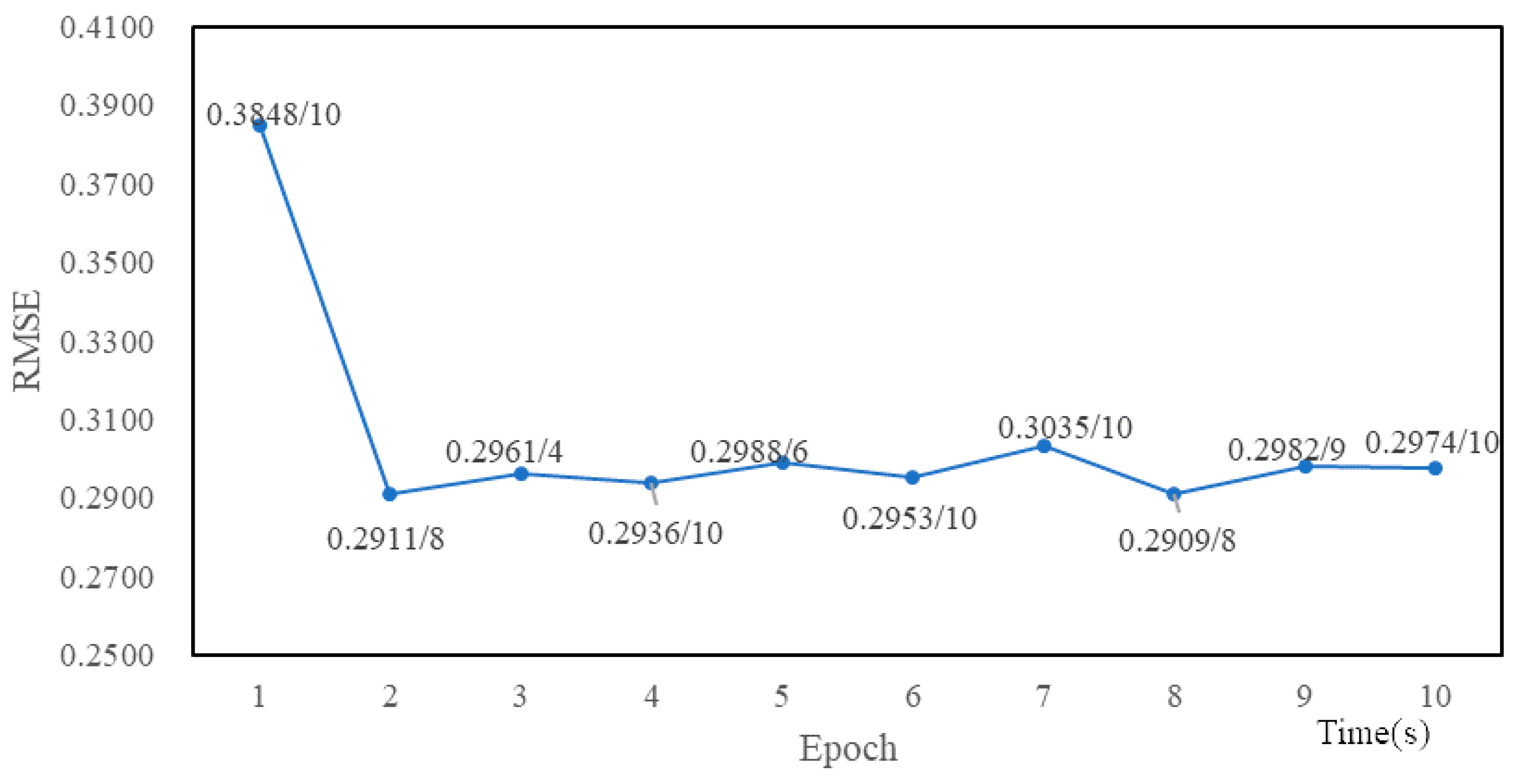
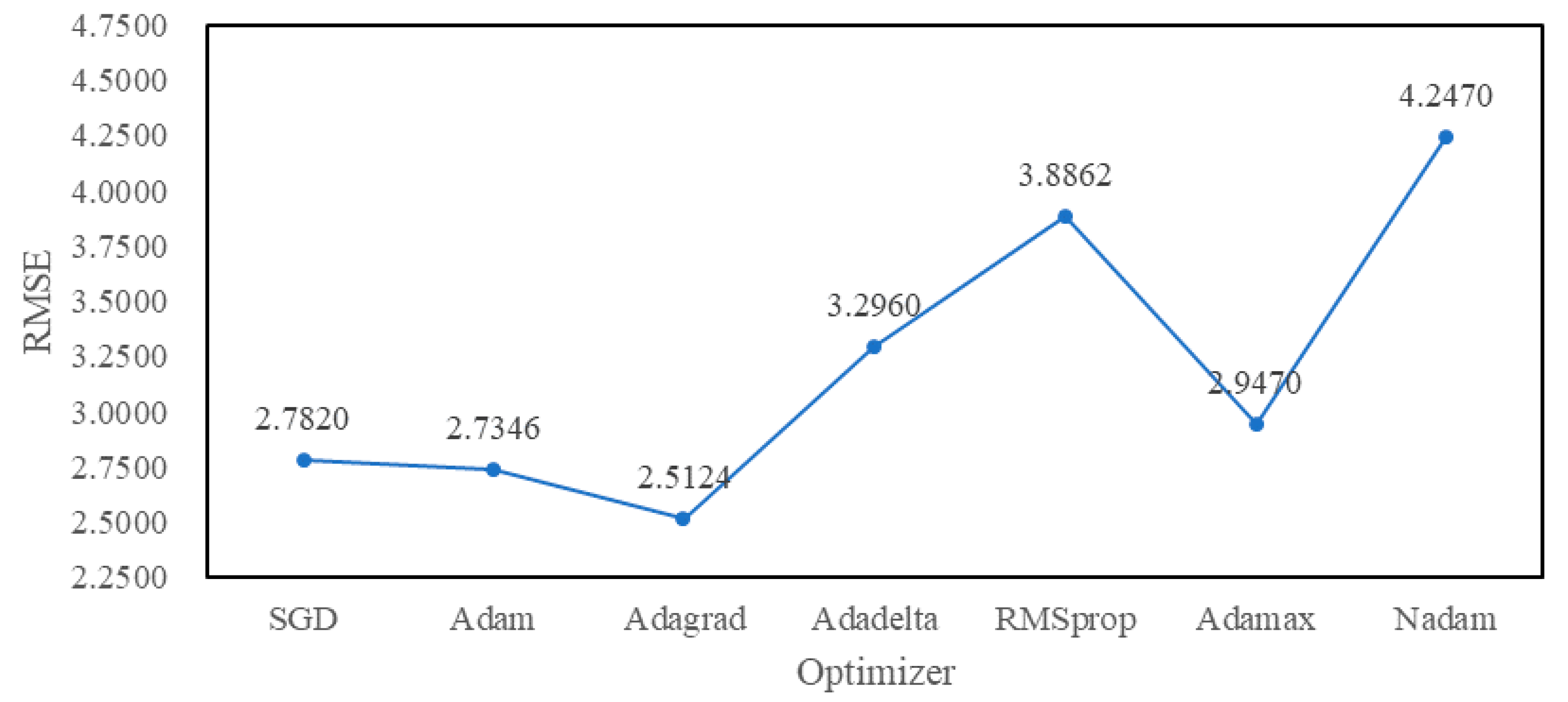
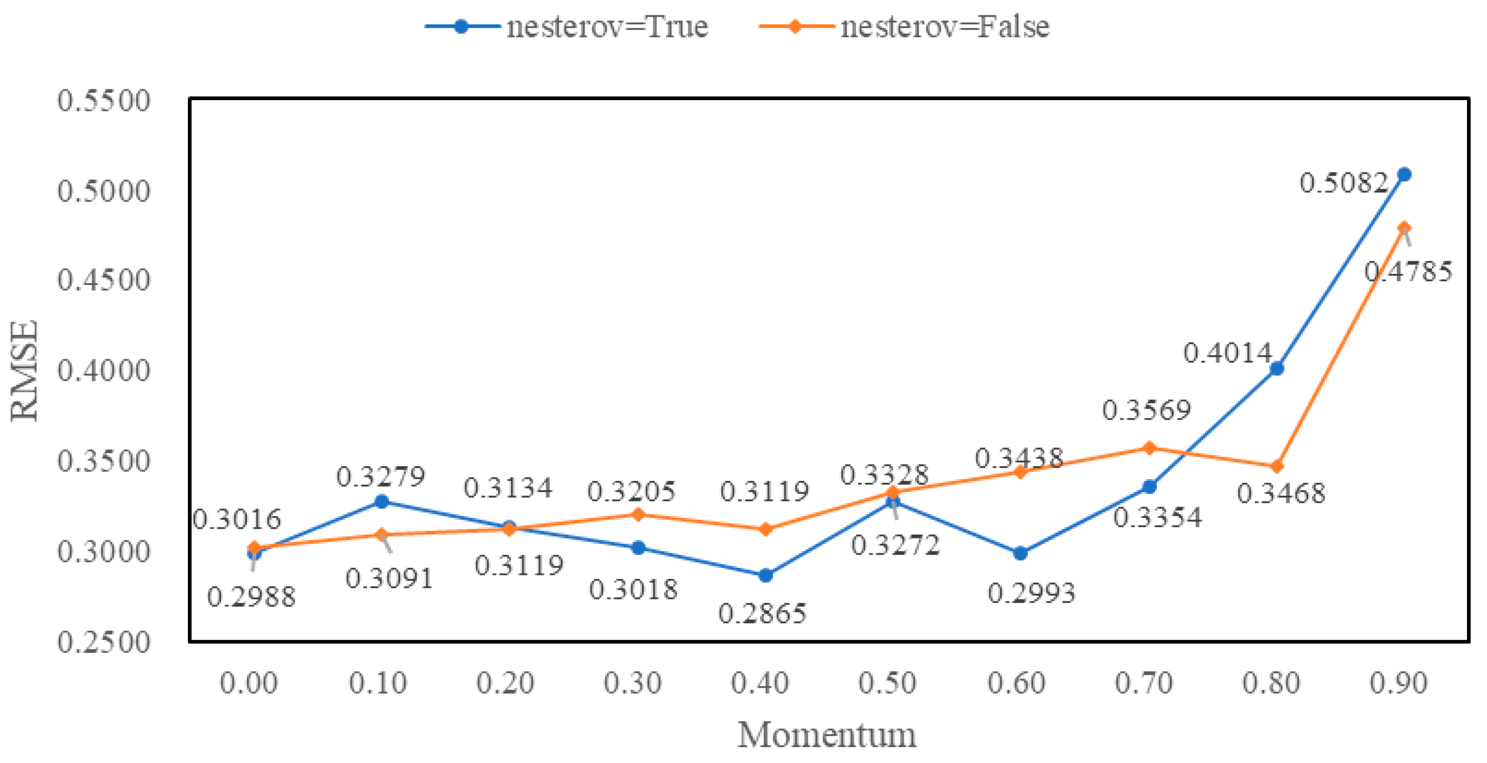
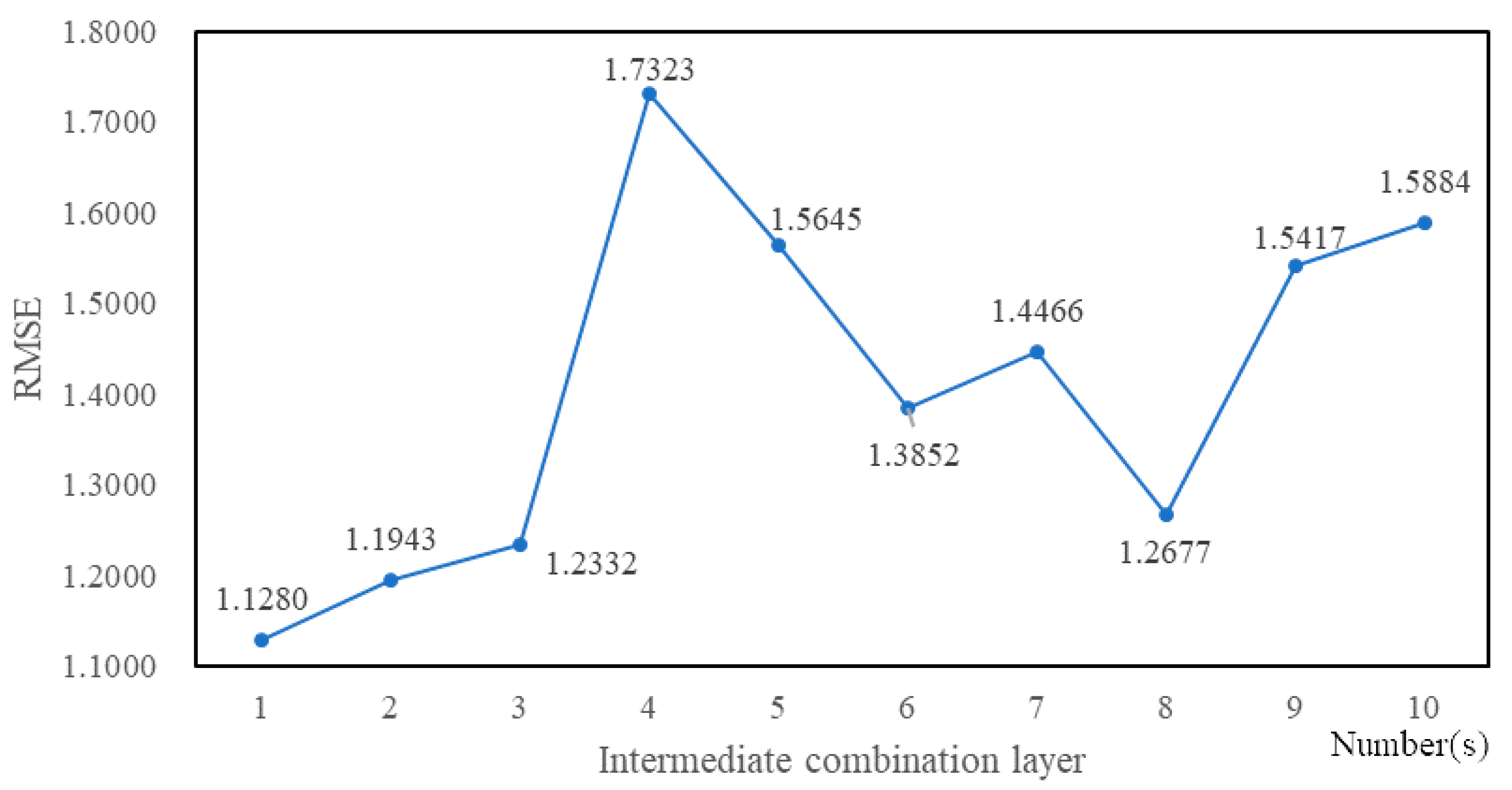
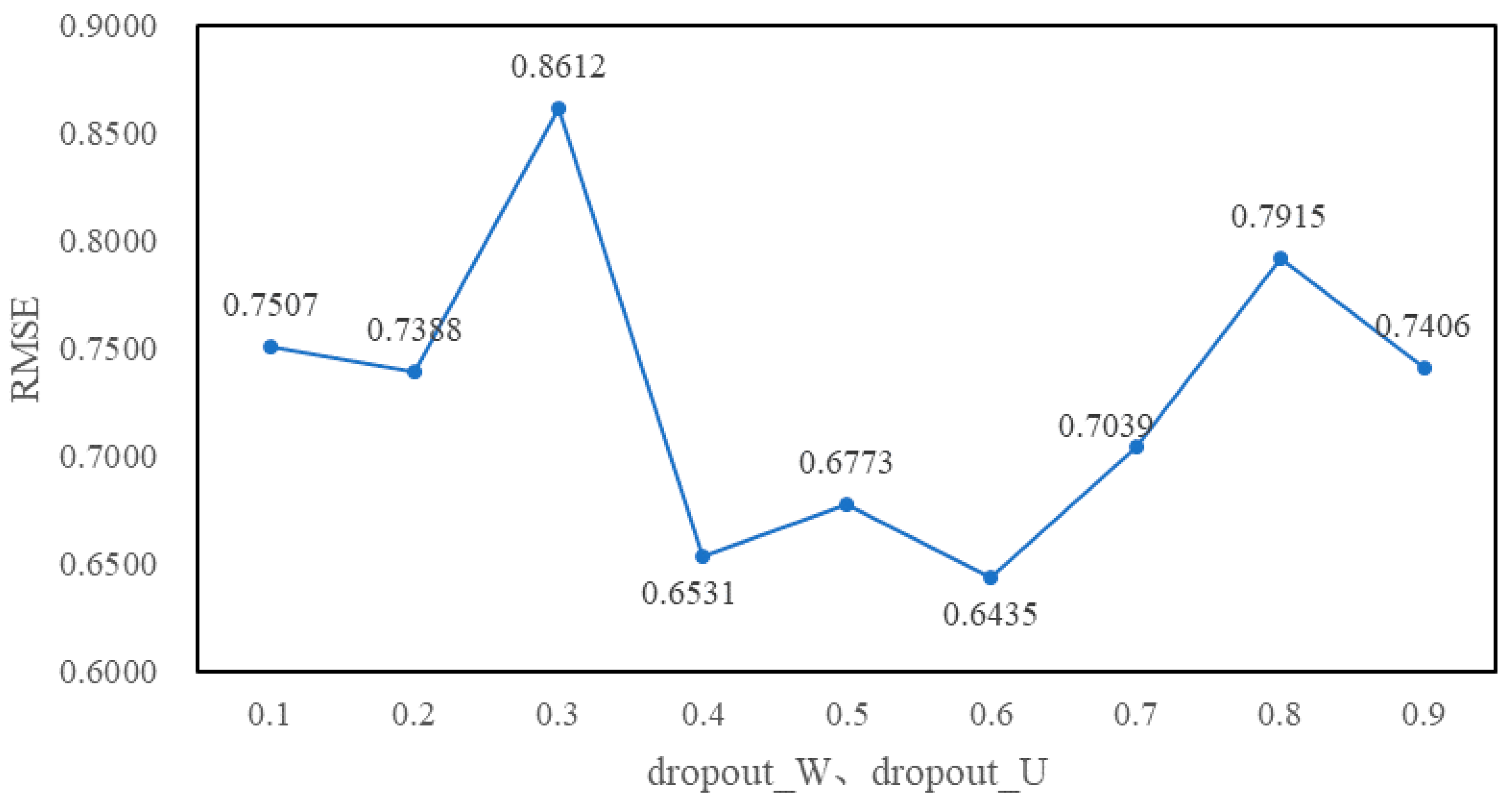
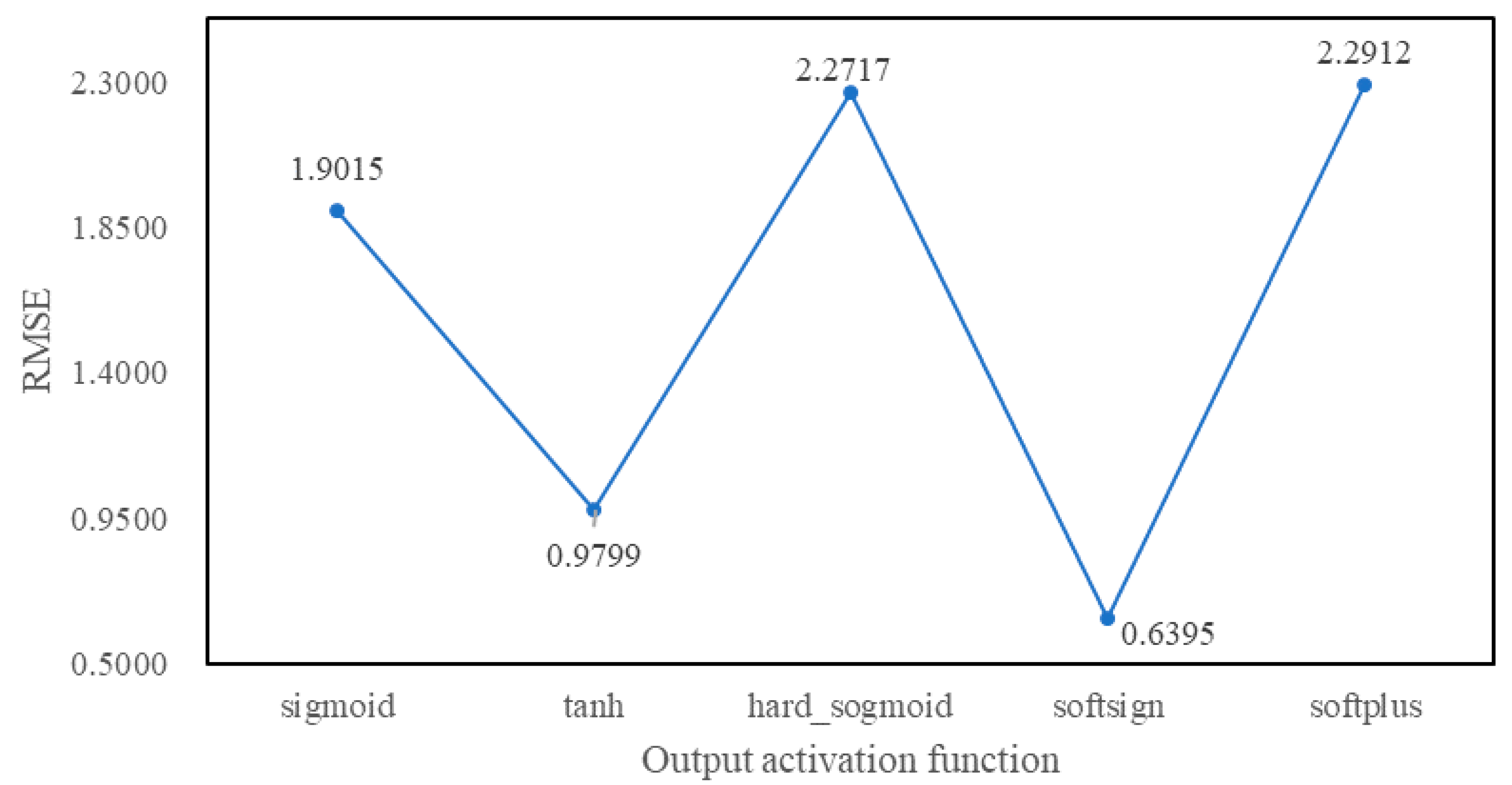
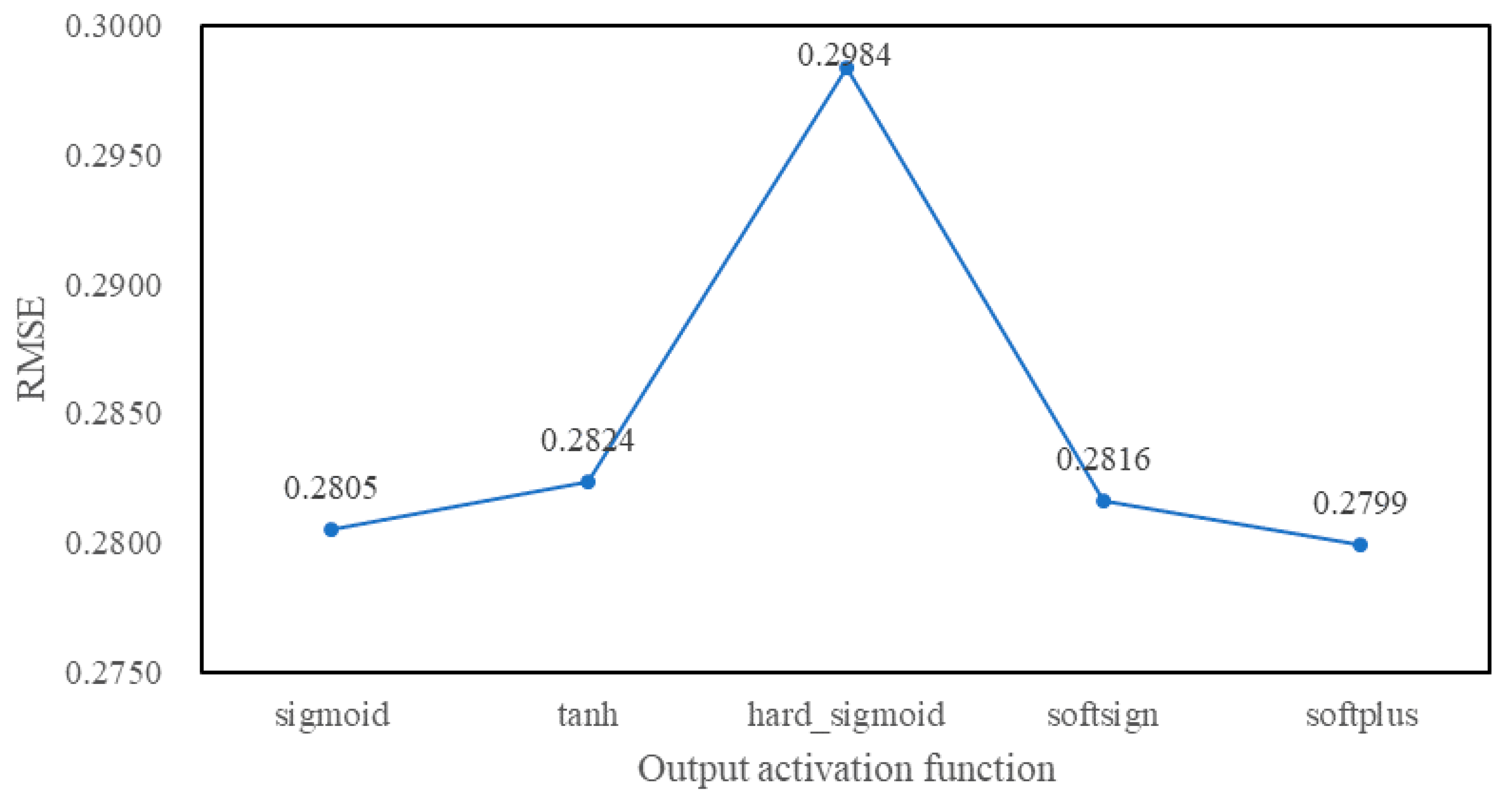
4.3. Experimental Tuning Process

In this paper, the process of optimization is based on the minimization principle and the layer-by-layer training method. The specific process is as follows.

(1) Data preprocessing

According to the actual traffic prediction requirements, the short-term traffic flow prediction of 5, 10 or 15 minutes is performed generally [38]. To get the finer granularity of the prediction value, this paper will take 5 minutes as time granularity to predict the future traffic flow based on the historical traffic flow. Therefore, we need to add up every ten-traffic data, and generate a new data set with three fields, i.e., Current Node, Source Node, and Traffic Flow with a matrix dimension of 168.

After statistical analysis of the traffic flow of all road sections, it is found that there are two types of road sections in the new data set, i.e., the road section with large traffic flow and the road section with small traffic flow respectively. For the section with large traffic flow, the traffic flow ranges from 150 to 200 during the rush hour, and from 10 to 100 during the rest of the sampling time. For the section with small traffic flow, the maximum traffic flow can only reach about 10 during the rush hour, and the traffic flow fluctuates between 0 and 2 during the rest of sampling time. Therefore, the new data set is divided into the large traffic flow data set and the small traffic flow data set.

To transform time series into supervised learning problems and evaluate the accuracy of model prediction, this paper divided the traffic flow data set (i.e., the large traffic flow data set or the small traffic flow data set) into training set and test set, where the first 70% (118 data) of the traffic flow data set is the training set and the last 30% (50 data) of the traffic flow data set is the test set. Training a model based the training set, the model will get 50 predictive values, and finally use RMSE to evaluate the prediction accuracy.

Data difference and data scaling are performed on the training set. Data difference adopts delay difference, namely difference transformation between continuous observation values which mainly eliminates some fluctuations. Because the default activation function of the LSTM model is tanh function, the output value range of this function is [−1, 1], so it is generally necessary to scale the data to the range of −1 to 1. However, considering that the traffic flow on any condition cannot be negative, we scale the training set to the range of 0 to 1. The data of the first day from tl8 to tl9 (or Sample1 for short) is selected from the large traffic flow data set, and the data of the first day (or Sample2 for short) from tl12 to tl11 is selected from the small traffic flow data set. The above two data sets will be used in the following experimental processes.

(2) Basic parameters tuning

Basic parameters tuning is mainly to tune the batch size (i.e., batch_size), the number of iterations (i.e., epoch) and the neurons number. When tuning the basic parameters in Keras, the hybrid LSTM neural network structure shown in Figure 1 only selects the LSTM layer, and the parameters of the LSTM layer are set to the default values. The batch_size represents the size of the batch and defines the number of samples that are propagated through the network. The batch_size is set to 1, making the model perform on-line learning. That is to say, the network will be updated after each training process. The epoch time and number of neurons are tuned through experiments as follows.

Firstly, we fix the time of epoch to 10 and tested the trend of RMSE when the number of neurons changed. The results are shown in Figure 4 and Figure 5.

Figure 4. RMSE values of Sample1 with different neurons numbers.

Figure 5. RMSE values of Sample2 with different neurons numbers.

According to Figure 4 and Figure 5, when the number of neurons is between 1 and 10, the RMSE value gradually decreases to the minimum and then increases with the increase of neurons number. And when the neurons number is greater than 10, the RMSE value continues to grow, and the running time becomes significantly longer. Therefore, in the following epoch time and neurons number tuning experiments, the neurons number for each epoch time is fixed between 1 and 10. The results are shown in Figure 6 and Figure 7.

Figure 6. The minimum RMSE values and corresponding neurons numbers for Sample1 with different epoch times.

Figure 7. The minimum RMSE values and corresponding neurons numbers for Sample2 with different epoch times.

According to Figure 6 and Figure 7, for Sample1, when the epoch time is 3 and the neurons number is 6, the RMSE value is the minimum. In other words, the optimal epoch time and neurons number for Sample1 are 3 and 6 respectively. For Sample2, when the epoch time is 8 and the neurons number is 8, the RMSE value is the minimum. Thus, the optimal epoch time and neurons number for Sample2 are 8 and 8 respectively.

(3) Optimizer tuning

The optimization problem is to find a set of parameters for a given objective function, so that the RMSE value is the minimum. The commonly used optimizers include Stochastic Gradient Descent (SGD), Adagrad, Adadelta, RMSprop, Adam, Adamax, Nadam, etc. [39]. When tuning the optimizes in Keras, the hybrid LSTM neural network structure shown in Figure 1 only selects the LSTM layer, and the parameters of the LSTM layer are set to the default values. And the above optimal batch size, epoch time and neurons number are applied here. Figure 8 and Figure 9 are the RMSE values of different optimizers for Sample1 and Sample2 respectively.

Figure 8. RMSE values of the different optimizers for Sample1.

Figure 9. RMSE values of the different optimizers for Sample2.

From Figure 8 and Figure 9, the RMSE value of Adagrad is the minimum for Sample1 when only the optimizer function is changed and the other parameters are kept as the initial default values. Similarly, the best optimizer for Sample2 is SGD. The learning rate of SGD generally has two values: 0.01 and 0.1, while the value of decay is generally 10⁻⁶. The RMSE value for Sample2 is 0.2875 when the learning rate of SGD is 0.01 and the RMSE value for Sample2 is 0.6786 when the learning rate of SGD is 0.1. Therefore, the learning rate of SGD for Sample2 is fixed at 0.01 in subsequent experiments. The momentum and nesterov values of SGD for Sample2 are then tested, as shown in Figure 10.

Figure 10. RMSE values of different momentum and nesterov values of Stochastic Gradient Descent (SGD) for Sample2.

From Figure 10, we can see that the RMSE value is the minimum when the momentum value is 0.4 and the nesterov value is True.

(4) Intermediate activation function tuning

The intermediate activation functions here refer to the activation functions of the Activation layers of both the input combination layer and intermediate combination layer in Figure 1, and the same activation function is usually selected. When tuning the intermediate activation functions in Keras, the hybrid LSTM neural network structure shown in Figure 1 only selects the LSTM layer and the Activation layer of the input combination layer, and the parameters of the LSTM layer are set to the default values. In addition, the other parameters are the optimal values of the above tuning results. Figure 11 and Figure 12 are the RMSE values of different activation functions for Sample1 and Sample2 respectively.

Figure 11. RMSE values of different intermediate activation functions for Sample1.

Figure 12. RMSE values of different intermediate activation functions for Sample2.

As shown in Figure 11 and Figure 12, there is the minimum RMSE value when the intermediate activation function is PReLU, whether Sample1 or Sample2. Hence, the intermediate activation function is set to PReLU in subsequent experiments.

(5) Network structure tuning

When tuning the network structure in Keras, the hybrid LSTM neural network structure shown in Figure 1 selects one input combination layer, zero or more intermediate combination layers and one output combination layer, where the parameters of the LSTM layer of the input combination layer are set to the default values, the parameters of the Dense layer of both the intermediate combination layer and the output combination layer are set to the default values, the activation functions of the Activation layers of both the input combination layer and the intermediate combination layer are set to PReLU function, the activation function of the Activation layer of the output combination layer is set to tanh function, and the dropout dates of the Dropout layers of both the input combination layer and the intermediate combination layer are set to 0.5. Figure 13 and Figure 14 are the RMSE values of different intermediate combination layer numbers for Sample1 and Sample2.

Figure 13. RMSE values of different intermediate combination layer numbers for Sample1.

Figure 14. RMSE values of different intermediate combination layer numbers for Sample2.

From Figure 13 and Figure 14, we can see that the RMSE value is the minimum when the number of intermediate combination layer is 1, regardless of Sample1 or Sample2. Therefore, the hybrid LSTM neural network structure shown in Figure 1 only selects one intermediate combination layer in the subsequent experiments.

(6) Dropout tuning

For the above hybrid LSTM neural network structure after tuning, the selection of dropout rate is mainly in both the LSTM layer and the Dropout layer of the input combination layer, and the Dropout layer of the intermediate combination layer. And the dropout rate of the Dropout layer of the intermediate combination layer is generally set to 0.5 [40]. To keep the input from changing too much, the dropout rate of the Dropout layer of the input combination layer is generally set to close to 1. Figure 15 is the RMSE values of the different dropout rates of the Dropout layer in the input combination layer for Sample1.

Figure 15. RMSE values of the different dropout rates of the Dropout layer in the input combination layer for Sample1.

From Figure 15, the RMSE value is the minimum for Sample1 when the dropout rate of the Dropout layer in the input combination layer is set to 0.9. Figure 16 is the RMSE values of the different dropout rates of the LSTM layer in the input combination layer for Sample1.

Figure 16. RMSE values of the different dropout rates of the LSTM layer in the input combination layer for Sample1.

According to Figure 16, the RMSE value is minimum for Sample1 when the values of both Dropout_W and Dropout_U of the LSTM layer in the input combination layer are set to 0.6. For Sample 2, the dropout rates of both the LSTM layer and the Dropout layer have no significant effect on RMSE. Therefore, in the subsequent experiments, the values of both Dropout_W and Dropout_U of the LSTM layer in the input combination layer are set to 0.6, while the dropout rate of the Dropout layer in the input combination layer is set to 0.9, whether Sample1 or Sample2.

(7) Output activation function tuning

The output activation function here refers to the activation function of the Activation layer of the output combination layer in Figure 1. Based on the above network structure and parameters selected, the output activation function is tuned in Keras. Figure 17 and Figure 18 are the RMSE values of different activation functions for Sample1 and Smaple2.

Figure 17. RMSE values of different output activation functions for Sample1.

Figure 18. RMSE values of different output activation functions for Sample2.

As we can see from Figure 17 and Figure 18, the RMSE value is the minimum when the output activation function is softsign for Sample1, while the RMSE value is the minimum when the output activation function is softplus for Sample2.

5. Experimental Results

According to the above experimental tuning process, for the Sample1, the optimal hybrid LSTM neural network structure is composed of an input combination layer, an intermediate combination layer and an output combination layer, where the batch_size value is 1, the epoch time is 3, the neurons number is 6, the optimizer is Adagrad, the activation functions of the Activation layers of both the input combination layer and the intermediate combination layer are PReLU, the activation function of the Activation layer in the output combination layer is the softsign, the values of both Dropout_W and Dropout_U of the LSTM layer in the input combination layer are 0.6, the dropout rate of the Dropout layer in the input combination layer is 0.9, the dropout rate of the Dropout layer in the intermediate combination layer is 0.5, and the other parameters are the default values in Keras.

For Sample2, the optimal hybrid LSTM neural network structure is composed of an input combination layer, an intermediate combination layer and an output combination layer, where the batch_size value is 1, the epoch time is 8, the neurons number is 8, the optimizer is SGD (the learning rate is 0.01, the momentum value is 0.4 and the nesterov value is True), the activation functions of the Activation layers of both the input combination layer and the intermediate combination layer are PReLU, the activation function of the Activation layer in the output combination layer is the softplus, the values of both Dropout_W and Dropout_U of the LSTM layer in the input combination layer are 0.6, the dropout rate of the Dropout layer in the input combination layer is 0.9, the dropout rate of the Dropout layer in the intermediate combination layer is 0.5, and the other parameters are the default values in Keras.

Through the above experimental optimization process, the final RMSE value for Smaple1 is reduced to 0.6395, while the final RMSE value for Smaple2 is reduced to 0.2799. For Sample1 and Sample2, the performance of the FCM model, the Kalman filter, the SVR model, the LSTM model and the above hybrid LSTM model are further compared, as shown in Table 2 and Table 3.

Table 2. The RMSE value and running time of different prediction models for Sample1.

Prediction Model	RMSE	Running Time (s)
FCM [25]	27.38	11.87
Kalman filter [6]	29.40	0.55
SVR [9]	15.04	0.50
LSTM [30]	31.57	4.04
hybrid LSTM	0.64	5.94

Table 3. The RMSE value and running time of different prediction models for Sample2.

Prediction Model	RMSE	Running Time (s)
FCM [25]	4.06	12.88
Kalman filter [6]	1.87	0.72
SVR [9]	1.23	0.19
LSTM [30]	2.38	4.21
Hybrid LSTM	0.28	7.60

From Table 2 and Table 3, we can see that our proposed hybrid LSTM model is obviously better than the other prediction models in prediction accuracy, and only slightly longer than the LSTM model in running time. Hence, our proposed hybrid LSTM model is reasonable and feasible.

To verify the effectiveness of the above hybrid LSTM model in the whole road network, the above hybrid LSTM model is further applied to each road section of the road network shown in Figure 3. Figure 19 is a thermodynamic diagram of the actual vehicle flow of each road section of the road network shown in Figure 3 from 18:00 p.m. to 18:05 p.m. The deeper the color, the greater the traffic flow.

Figure 19. The thermodynamic diagram of the actual vehicle flow of each road section of the road network shown in Figure 3 from 18:00 p.m. to 18:05 p.m.

In Figure 19, the actual vehicle flows of two directions are marked at each road section of the road network. Figure 20 shows the predictive vehicle flow of each road section of the road network shown in Figure 3 from 18:00 p.m. to 18:05 p.m.

Figure 20. The thermodynamic diagram of the predictive vehicle flow of each road section of the road network shown in Figure 3 from 18:00 p.m. to 18:05 p.m.

In Figure 20, the absolute errors between the actual and predictive vehicle flows of both directions are marked at each road section of the road network. Because the vehicle flow at a road intersection is formed by the vehicle flows of the connected road sections, the actual and predictive vehicle flows of a road intersection can be calculated according to the actual and predictive vehicle flows of the connected road section. Figure 21 is a thermodynamic diagram of the actual vehicle flow of each road intersection of the road network shown in Figure 3 from 18:00 p.m. to 18:05 p.m. The deeper the color and the larger the color block in the circle, the greater the traffic flow.

Figure 21. The thermodynamic diagram of the actual vehicle flow of each road intersection of the road network shown in Figure 3 from 18:00 p.m. to 18:05 p.m.

In Figure 21, the actual vehicle flow is marked at each road intersection of the road network. Figure 22 shows the predictive vehicle flow of each road intersection of the road network shown in Figure 3 from 18:00 p.m. to 18:05 p.m.

Figure 22. The thermodynamic diagram of the predictive vehicle flow of each road intersection of the road network shown in Figure 3 from 18:00 p.m. to 18:05 p.m.

In Figure 22, each intersection in the road network is marked with the absolute error between the actual and predictive vehicle flow. According to Figure 20 and Figure 22, the maximum relative error between the actual and predictive vehicle flows of each road section is 1.03%, and the maximum relative error between the actual and predictive vehicle flows of each road intersection is 1.18%. Therefore, the above hybrid LSTM model has a very high prediction accuracy, so it is very effective.

6. Conclusions

The prediction accuracy of the existing short-term traffic flow prediction models is still low, and they are not suitable for different traffic conditions of the actual traffic network. To solve these problems, a hybrid LSTM neural network is proposed based on the LSTM model in this paper. It consists of one input combination layer, zero or more intermediate combination layers and one output combination layer. The input combination layer includes a LSTM layer, an Activation layer and a Dropout layer, the intermediate combination layer includes a Dense layer, an Activation layer and a Dropout layer, and the output combination layer includes a Dense layer and an Activation layer. Then, the structure and parameters of the hybrid LSTM neural network are optimized for the large traffic flow set and the small traffic flow set. The results show that the RMSE value of the hybrid LSTM model is obviously smaller than the other typical models, and the running time is only slightly longer than the LSTM model. Thus, the hybrid LSTM model is closer to the accuracy and real-time requirements of short-term traffic flow prediction. Finally, the hybrid LSTM model is further used to predict the vehicle flows of each road section and intersection in the actual traffic network. The results show that the maximum relative error between the actual and predictive vehicle flows of each road section is 1.03%, and the maximum relative error between the actual and predictive vehicle flows of each road intersection is 1.18%. Hence, the hybrid LSTM model has a very high prediction accuracy, and suitable for different traffic conditions in the actual traffic network.

Running time is also important for short-term traffic flow prediction. We will further study the variant of the LSTM model, making its accuracy is essentially equivalent to the accuracy of the hybrid LSTM model, but its running time is shorter than the running time of the hybrid LSTM model. Additionally, this work is based on traffic flow data. In a future study, we will further research the prediction and analysis of traffic trajectory data.

References

1. Okutani, I.; Stephanedes, Y.J. Dynamic prediction of traffic volume through kalman filtering theory. Transp. Res. Part B Methodol. 1984, 18, 1–11. [Google Scholar] [CrossRef]
2. Perera, L.P.; Soares, C.G. Ocean vessel trajectory estimation and prediction based on extended kalman filter. In Proceedings of the Second International Conference on Adaptive and Self-Adaptive Systems and Applications, Lisbon, Portugal, 14–20 November 2010. [Google Scholar]
3. Chen, C.; Hu, J.; Meng, Q.; Zhang, Y. Short-time traffic flow prediction with ARIMA-GARCH model. In Proceedings of the 2011 IEEE Intelligent Vehicles Symposium (IV), Baden-Baden, Germany, 5–9 June 2011; pp. 607–612. [Google Scholar]
4. Shen, G.; Zhu, Y. Short-term traffic flow forecasting based on hybrid model. J. Nanjing Univ. Technol. 2014, 38, 246–251. [Google Scholar]
5. Zhu, Z.; Liu, L.; Cui, M. Short-term traffic flow forecasting model combining SVM and kalman filter. Comput. Sci. 2013, 40, 248–251. [Google Scholar]
6. Yang, G.; Xu, R.; Qin, M.; Zheng, K.; Zhang, B. Short-term traffic volume forecasting based on ARMA and kalman filter. J. Zhengzhou Univ. (Eng. Sci.) 2017, 38, 36–40. [Google Scholar]
7. Tang, J.; Xu, G.; Wang, Y.; Wang, H.; Zhang, S.; Liu, F. Traffic flow prediction based on hybrid model using double exponential smoothing and support vector machine. In Proceedings of the 16th International IEEE Conference on Intelligent Transportation Systems (ITSC 2013), Hague, The Netherlands, 6–9 October 2013; pp. 130–135. [Google Scholar]
8. Li, S.; Liu, L.; Zhai, M. Prediction for short-term traffic flow based on modified PSO optimized BP neural network. Syst. Eng. Theory Pract. 2012, 32, 2045–2049. [Google Scholar]
9. Liu, J. Short-term traffic flow prediction model of phase space reconstruction and support vector regression with combination optimization. Comput. Eng. Appl. 2014, 50, 13–17. [Google Scholar]
10. Gao, S. Short time traffic flow prediction model based on neural network and cuckoo search algorithm. Comput. Eng. Appl. 2013, 49, 106–109. [Google Scholar]
11. Zhang, J.; Wang, Y.; Zhu, X. Short-term prediction of traffic flow based on neural network optimized improved particle swarm optimization. Comput. Eng. Appl. 2017, 53, 227–231. [Google Scholar]
12. Hou, Y.; Zhao, H. Traffic flow prediction based on T-S fuzzy neural network optimized improved particle swarm optimization. Comput. Eng. Appl. 2014, 50, 236–239. [Google Scholar]
13. Shen, Y.; Yan, J.; Wang, W. Short-term traffic flow forecasting based on WNN optimized by CPSO. Comput. Appl. Softw. 2014, 31, 84–90. [Google Scholar]
14. Zang, Y.; Ni, F.; Feng, Z.; Cui, S.; Ding, Z. Wavelet transform processing for cellular traffic prediction in machine learning networks. In Proceedings of the 2015 IEEE China Summit and International Conference on Signal and Information Processing (ChinaSIP), Chengdu, China, 12–15 July 2015; pp. 458–462. [Google Scholar]
15. Minal, D.; Preeti, R.B. Short term traffic flow prediction based on neuro-fuzzy hybrid system. In Proceedings of the 2016 IEEE International Conference on ICT in Business Industry & Government (ICTBIG), Indore, India, 1–3 November 2016. [Google Scholar]
16. Kumar, A. Novel multi input parameter time delay neural network model for traffic flow prediction. In Proceedings of the 2016 IEEE Online International Conference on Green Engineering and Technologies (IC-GET), Coimbatore, India, 1–6 November 2016. [Google Scholar]
17. Yu, B.; Duan, X.; Wu, Y. Establishment and application of data prediction model based on BP neural network. Comput. Digit. Eng. 2016, 44, 482–486. [Google Scholar]
18. Zhang, C.; Liu, S.; Tan, T. Research on short-term traffic flow prediction methods based on modified genetic algorithm optimized BP neural network. J. Tianjin Chengjian Univ. 2017, 23, 143–148. [Google Scholar]
19. Zhang, Q.; Zhu, X. Short-term traffic flow forecasting method based on GA-elman neural network. J. Lanzhou Univ. Technol. 2013, 39, 95–98. [Google Scholar]
20. Yi, H.; Jung, H.; Bae, S. Deep neural networks for traffic flow prediction. In Proceedings of the 2017 IEEE International Conference on Big Data and Smart Computing (BigComp), Jeju, Korea, 13–16 February 2017; pp. 328–331. [Google Scholar]
21. Yin, L.; He, Y.; Dong, X.; Lu, Z. Research on the multi-step prediction of volterra neural network for traffic flow. Acta Autom. Sin. 2014, 40, 2066–2072. [Google Scholar]
22. Emilian, N. Dynamic traffic flow prediction based on GPS data. In Proceedings of the 2014 IEEE 26th International Conference on Tools with Artificial Intelligence (ICTAI), Limassol, Cyprus, 10–12 November 2014; pp. 922–929. [Google Scholar]
23. Surya, S.; Rakesh, N. Flow based traffic congestion prediction and intelligent signaling using markov decision process. In Proceedings of the 2016 IEEE International Conference on Inventive Computation Technologies (ICICT), Coimbatore, India, 1–6 August 2016. [Google Scholar]
24. Luo, X.; Jiao, Q.; Niu, L.; Sun, Z. Short-term traffic flow prediction based on deep learning. Appl. Res. Comput. 2017, 34, 91–97. [Google Scholar]
25. Zhang, M. Short-term traffic flow prediction of non-detector intersections based on FCM. Comput. Technol. Dev. 2017, 27, 39–45. [Google Scholar]
26. Rui, L.; Li, Q. Short-term traffic flow prediction algorithm based on combined model. J. Electron. Inf. Technol. 2016, 38, 1227–1233. [Google Scholar]
27. Pascale, A.; Nicoli, M. Adaptive bayesian network for traffic flow prediction. In Proceedings of the 2011 IEEE Statistical Signal Processing Workshop (SSP), Nice, France, 28–30 June 2011; pp. 177–180. [Google Scholar]
28. Wen, M.; Yu, W.; Peng, J.; Zhang, X. A traffic flow prediction algorithm based on adaptive particle filter. In Proceedings of the 2014 26th Chinese Control and Decision Conference (CCDC), Changsha, China, 31 May–2 June 2014; pp. 4736–4740. [Google Scholar]
29. Borkowski, P. The ship movement trajectory prediction algorithm using navigational data fusion. Sensors 2017, 17, 1432. [Google Scholar] [CrossRef]
30. Shao, H.; Soong, B.H. Traffic flow prediction with long short-term memory networks (LSTMs). In Proceedings of the 2016 IEEE Region 10 Conference (TENCON), Singapore, 22–25 November 2016; pp. 2986–2989. [Google Scholar]
31. Lipton, Z.C. A Critical Review of Recurrent Neural Networks for Sequence Learning. Available online: https://arxiv.org/pdf/1506.00019v2.pdf (accessed on 2 February 2019).
32. Hochreiter, S.; Schmidhuber, J. Long short-term memory. Neural Comput. 1997, 9, 1735–1780. [Google Scholar] [CrossRef]
33. Graves, A. Supervised Sequence Labelling with Recurrent Neural Networks Book; Springer: Berlin/Heidelberg, Germany, 2012; pp. 31–38. [Google Scholar]
34. He, K.; Zhang, X.; Ren, S.; Sun, J. Delving Deep into Rectifiers: Surpassing Human-Level Performance on ImageNet Classification. Available online: https://arxiv.org/pdf/1502.01852.pdf (accessed on 18 February 2019).
35. Xavier, G.; Yoshua, B. Understanding the difficulty of training deep feedforward neural networks. J. Mach. Learn. Res. 2010, 9, 249–256. [Google Scholar]
36. Xavier, G.; Yoshua, B.; Bengio, Y. Deep sparse rectifier neural networks. J. Mach. Learn. Res. 2011, 15, 315–323. [Google Scholar]
37. Krizhevsky, A.; Sutskever, I.; Hinton, G.E. Imagenet classification with deep convolutional neural networks. In Proceedings of the 26th Annual Conference on Neural Information Processing Systems, Lake Tahoe, NV, USA, 3–6 December 2012; pp. 1097–1105. [Google Scholar]
38. Wang, W.; Guo, X. Jiaotong Gongchengxue, 1st ed.; Southeast University Press: Nan Jing, China, 2000; p. 37. ISBN 7-81050-680-3. [Google Scholar]
39. Keras Documentation. Available online: https://keras.io/ (accessed on 2 February 2019).
40. Srivastava, N.; Hinton, G.; Krizhevsky, A.; Sutskever, I.; Salakhutdinov, R. Dropout: A simple way to prevent neural networks from overfitting. J. Mach. Learn. Res. 2014, 15, 1929–1958. [Google Scholar]
Article Metrics
Citations
Article Access Statistics
Multiple requests from the same IP address are counted as one view.