Article

DFTHR: A Distributed Framework for Trajectory Similarity Query Based on HBase and Redis

College of Electronic Engineering, Naval University of Engineering, Wuhan 430033, China
*
Author to whom correspondence should be addressed.
Information 2019, 10(2), 77; https://doi.org/10.3390/info10020077
Submission received: 12 January 2019 / Revised: 15 February 2019 / Accepted: 21 February 2019 / Published: 24 February 2019
(This article belongs to the Section Information Systems)

Abstract

:
In recent years positioning sensors have become ubiquitous, and there has been tremendous growth in the amount of trajectory data. It is a huge challenge to efficiently store and query massive trajectory data. Among the typical operation over trajectories, similarity query is an important yet complicated operator. It is useful in navigation systems, transportation optimizations, and so on. However, most existing studies have focused on handling the problem on a centralized system, while with a single machine it is difficult to satisfy the storage and processing requirements of mass data. A distributed framework for the similarity query of massive trajectory data is urgently needed. In this research, we propose DFTHR (distributed framework based on HBase and Redis) to support the similarity query using Hausdorff distance. DFTHR utilizes a segment-based data model with a number of optimizations for storing, indexing and pruning to ensure efficient querying capability. Furthermore, it adopts a bulk-based method to alleviate the cost for adjusting partitions, so that the incremental dataset can be efficiently supported. Additionally, DFTHR introduces a co-location-based distributed strategy and a node-locality-based parallel query algorithm to reduce the inter-worker cost overhead. Experiments show that DFTHR significantly outperforms other schemes.

1. Introduction

With the rapid development of mobile networks and position technologies, trajectory data of moving object (MO) can be collected more easily and accurately. For example, a large ship reports its geo-location every few seconds through an AIS (automatic identification system) [1], and a DiDi taxi regularly uploads its real-time location by the related application. As a result, massive amounts of trajectory data are collected from different domains, and it is necessary to implement effective storage, query and analysis of the data.
There are many different, useful query operations over the trajectory datasets, such as range query, trajectory-to-point neighbor query, and so on. Among the many query operations, trajectory similarity query is an important basic query operator [2]. Its goal is to find one or more trajectories which similar to a query trajectory. This is useful in navigation systems, mobile applications and transportation optimizations, and is also the groundwork of many data-mining tasks such as classification and clustering.
However, most of the existing schemes [3,4,5,6,7,8] focus on solving the trajectory similarity query problem on a single machine, when processing similarity queries for massive data, and these schemes face inconceivable storage and process capability challenges. Moreover, it is difficult to directly apply these schemes to the distributed environment because they do not consider the impact of data transmission and load balance on queries.
In order to process the similarity query problem of large-scale trajectory data, some distributed framework based schemes [9,10,11,12] are proposed according to the selected distance functions. However, most of them [9,11,12] only support the static datasets, while in many real-life trajectory applications, the data is incrementally appended, and these schemes are difficult to apply directly. When each new batch of data arrives, these schemes should repartition all data from scratch, which leads to an expensive processing cost, and sacrifices flexibility and efficiency. Moreover, most of the above schemes [9,10,11] do not consider the effect of data transmission on queries, and they distribute the sub-trajectories and index data of the same MO in different partitions on different machines. In query processing, a large amount of across-node network overhead is required to handle the merger of the index or trajectory data.
In light of that, using Hausdorff distance [13] as the distance function, we propose DFTHR, a distributed framework for trajectory similarity query based on HBase [14] and Redis [15]. First, in order to accelerate query processing, we design a trajectory segment-based storage and index structure, and implement a trajectory segment-based pruning method to filter out the dissimilar trajectories. Second, we proposes a bulk-based partitioning model to deploy trajectory data and indexes in a distributed environment, and on this basis implement the mechanism of cost optimization to efficiently process the state change of each partitions so that our scheme can effectively support the incremental datasets. Finally, we devise certain maintenance strategies to ensure co-location between each partition and its corresponding index, and implement node-locality-based parallel query algorithms to reduce the data transmission overhead when querying. Our main contributions can be summarized as follows:
  • We propose a segment-based data model for storing and indexing trajectory data, which ensures efficient pruning and querying capacity.
  • We introduce a bulk-based partitioning model and certain optimization strategies to alleviate the cost of adjusting data distribution, so that an incremental dataset can be supported efficiently.
  • We design certain strategies to ensure the co-location between each partition and its corresponding index, and implement node-locality-based parallel query algorithms to reduce the inter-worker cost overhead when querying.
  • We evaluate our scheme with the dataset of ship trajectory, and the experimental results verify the efficiency.
Section 2 introduces the related work. The preliminaries about the problem formulation, the basics in HBase and Redis is introduced in Section 3. The structure of DFTHR is described in Section 4. Section 5 provides an experimental study of our system. Finally, we give a brief conclusion in Section 6.

2. Related Work

At present, the widely adopted distance functions for trajectory similarity can be classified as the metric ones like the Hausdorff distance [13] and Fréchet distance [16], and the non-metric ones like dynamic time warping (DTW) [17], the extended Frobenius norm (EROS) [18], the longest common subsequence (LCSS) [19] and the edit distance on real sequence (EDR) [20]. In many distance functions, the Hausdorff distance is one of the most general and widely adopted distance measures, so we develop the similarity query research based on the Hausdorff distance.
In order to boost the performance of trajectory similarity query, various pruning techniques are proposed according to the selected distance function. Morse et al. [3] propose a fast time series evaluation (FTSE) scheme which can be used to compute the threshold value of DTW, EDR and LCSS in a faster way. Bai et al. [4] boost the calculation efficiency of Hausdorff distance through computing this distance based on the consecutive fold lines and combining the two pruning strategies for the useless fold line segments. Zhu et al. [5] and Zhou et al. [6] use the piecewise cumulative approximation method (PAA) to transform the data into spatial vector points organized by R-Tree, and improve the compactness of the lower bound of DTW by certain methods respectively to improve spatial index pruning efficiency. Ranu et al. [7] extend edit distance to implement a distance function called edit distance with projections (EDwP) to support more accurate measure, and propose an index structure named TrajTree which employs the unique combination of bounding boxes with Lipschitz embedding to support this distance function. Zheng et al. [8] propose an in-memory frame structure to support the management of massive trajectory data, and implement support for trajectory similarity query based on sliding window and MBR. However, these schemes are designed for a stand-alone environment, and extending them to work in a distributed environment is not an easy task.
With the rapid development of distributed computing, various distributed frameworks are adopted by more and more schemes to process the similarity query of massive trajectory data.
Peixoto et al. [9] propose Voronoi pages to organize and partition trajectory data, and implement VSI (Voronoi Spatial Index) and TPI (Time Page Index) index structure to effectively prune the search space. In addition, they design a MapReduce algorithm based on the Spark RDD (resilient distributed datasets) structure to provide support for k-NN query of trajectory similarity.
Zhang et al. [10] propose a distributed in-memory system TrajSpark, which offers efficient management for mass trajectory data. It uses IndexTRDD to provide efficient compression storage and parallel query support, and tracts changes in data distribution through the time decay model to continuously support efficient management over the increasing mass trajectory data. Xie et al. [11] use a distributed in-memory system named SIMBA (Efficient In-Memory Spatial Analytics) [21] to solve the k-NN query problem of trajectory similarity and support two distance functions of the extended Hausdorff and extended Fréchet. It builds global and local indexes based on trajectory segments and uses bitmap and dual indexing to improve search performance. Shang et al. [12] design a distributed in-memory trajectory analytics prototype system called DITA (Distributed In-Memory Trajectory Analytics) based on Spark. It implements communication overhead optimization during the query process and supports a more compact lower bound for the distance functions of DTW, Fréchet, EDR, and LCSS. Moreover, based on a hybrid index structure, DITA achieves efficient support for threshold-based query and joint query.
Our work differs from them in two aspects. (1) Most previous schemes [9,11,12] only support the static datasets, but do not support the incremental datasets well. In real applications, data are often loaded in batches according to specific rules. When each batch arrives, these schemes should repartition both the existing and the new batch of data, which leads to an expensive processing cost. While our scheme supports a bulk-based partitioning model and certain optimization strategies to alleviate the cost of repartitioning, so that the incremental dataset can be supported efficiently. (2) Most of above schemes [9,10,11] do not consider the effect of data transmission on queries, they distribute the sub-trajectories and index data of the same MO in different partitions on different machines, and additional across-node network overhead is required during the query to handle the merger of the index or trajectory data of the same MO. While our scheme stores the data of the same MO in a partition, co-resides each partition and its corresponding index on the same node, and implements node-locality-based parallel query algorithms to reduce the data transmission overhead, thereby improving query efficiency.

3. Preliminary

3.1. Problem Formulation

Trajectory data is generated by sampling the spatiotemporal position of MOs. In this paper, we define the trajectory data as follows:
Definition 1.
A trajectory point p is a location-based data element, denoted as <moid, l, t, o>, where moid is the moving object identifier (MOID), l and t represent the spatial and timestamp information respectively, and o is the other information which includes speed, orientation, destination, etc.
Definition 2.
A trajectory T contains a sequence of trajectory points (p1, …, pm) orderly by their timestamps, and all points of T belong to the same MO.
Definition 3.
A trajectory segment TS contains the trajectory points of an MO sampled in a TI (Time Interval). Where TI is generated by unified division in time dimension, namely all the TIs are of the same length, so the start time of a TI can be its identifier. From the definition it is easy to know that a trajectory segment can be uniquely identified by MOID and TI attributes.
Figure 1 gives the examples of 4 2-dimensional trajectories (1 spatial + 1 temporal). Let TSxy be the trajectory segment of trajectory Tx in time interval TIy. As can be seen from the figure, trajectory T1 is composed of trajectory segments TS11, TS12, TS13 and TS14, and the trajectory T3 is composed of the trajectory segments TS31, TS32 and TS34 because there is no sampled point in time interval TI2.
Hausdorff distance is the farthest of all the distances from a point in one trajectory to the closest point in the other trajectory. It includes both the one-sided Hausdorff distance and the two-sided Hausdorff distance, as defined below:
Definition 4.
Given two trajectories TA = (pa1, …, pam) and TB=(pb1, …, pbn), one-sided Hausdorff distance is computed as below:
h ( T A , T B ) = max p a 1 T A min p b j T B p a i . l p b j . l , 1 i m , 1 j n ,
where pai.l and pbj.l are the spatial coordinates of pai and pbj respectively, p a i . l p b j . l is the point-to-point spatial distance between pai and pbj, we use Euclidean distance to measure the point-based spatial distance [13].
Definition 5.
Given two trajectories TA and TB, the two-sided Hausdorff distance from TA to TB is as follows:
H ( T A , T B ) = max [ h ( T A , T B ) , h ( T B , T A ) ] .
Namely the two-sided Hausdorff distance between TA and TB is the larger of the one-sided Hausdorff distance from TA to TB and the one-sided Hausdorff distance from TB to TA [13].
We use the two-sided Hausdorff distance as the distance function of similarity query. In the following text, whenever “Hausdorff distance” is mentioned, it defaults to the two-sided Hausdorff distance.
In the paper, we aim to solve the problems of trajectory similarity query. The two types of similarity queries we have designed for our scheme are the following:
Definition 6.
Given a time range trq, a query trajectory Tq, a distance threshold ε and a collection of trajectories TC = {T1, T2, …, Tn}, according to the Hausdorff distance, the threshold-based query of trajectory similarity returns the collection of trajectories TCq from TC and for any Ta ∈ TCq, H(Ta,Tq) ≤ ε.
Definition 7.
Given a time range trq, a query trajectory Tq and a collection of trajectories TC = {T1, T2, …, Tn}, according to the Hausdorff distance, the k-NN query of trajectory similarity finds the k trajectories from TC which are most similar to Tq within trq.

3.2. HBase

HBase is an open source distributed key-value database. It stores the data of a table over a cluster of nodes in a dispersed way to provide scalable storage to massive data. Data in HBase is stored in tables, and each data cell is indexed by rowkey, column family, column qualifier and time stamp. Among them, rowkey is the unique index for directly accessing data, it is closely related to data storage and query efficiency, and plays a very important role in data processing.
On the physical structure, HBase uses Region as the basic element for distributed storage (namely partition). An HBase table is usually divided horizontally into multiple Regions distributed in all data nodes (named as RegionServer), each Region stores a certain range of data rows. A Region should be split when its data scale is beyond the threshold, in order to make the data distribution of Regions more uniform [22].
In order to leverage the parallelism of HBase cluster, a co-processor mechanism that is similar to MapReduce framework is introduced. It can be divided into two kinds of Observer and Endpoint, whereby the Observer provides event hooks of table operation to capture and process certain events, and Endpoint provides the possibility for users to execute arbitrary code remotely in RegionServers [23].

3.3. Redis

Redis is an open source in-memory key-value database. All Redis data is typically held in memory, and is written to disk asynchronously from time to time to achieve persistent storage. Redis maps keys to types of values. An important character is that Redis supports not only strings, but also abstracts data types:
Redis String: Redis String is the most basic data type of Redis, namely a key corresponds to a string value.
Redis Hash: a map table to store associated field-value pairs under a unique key, where both the fields and values are strings.
Redis List: a simple list of strings sorted by insertion order, the elements can be added to the head or the tail of a Redis List.
Redis Set: an unordered collection of unique strings, it is implemented by hash table, so the complexity of adding, deleting, and finding is O(1).
Redis Sorted Set: like Redis Set, this is also a string set with the unique feature. The difference is that that each element is associated with a double type of score, and ordering is according to scores and the string lexicographical order.
Early Redis versions can only be deployed in stand-alone mode. In version 3.0, the clustering model for Redis is introduced, A Redis cluster is able to scale up to thousands of nodes to provide quality, efficient and scalable storage services [24].

4. Distributed Framework Based on HBase and Redis (DFTHR) Structure
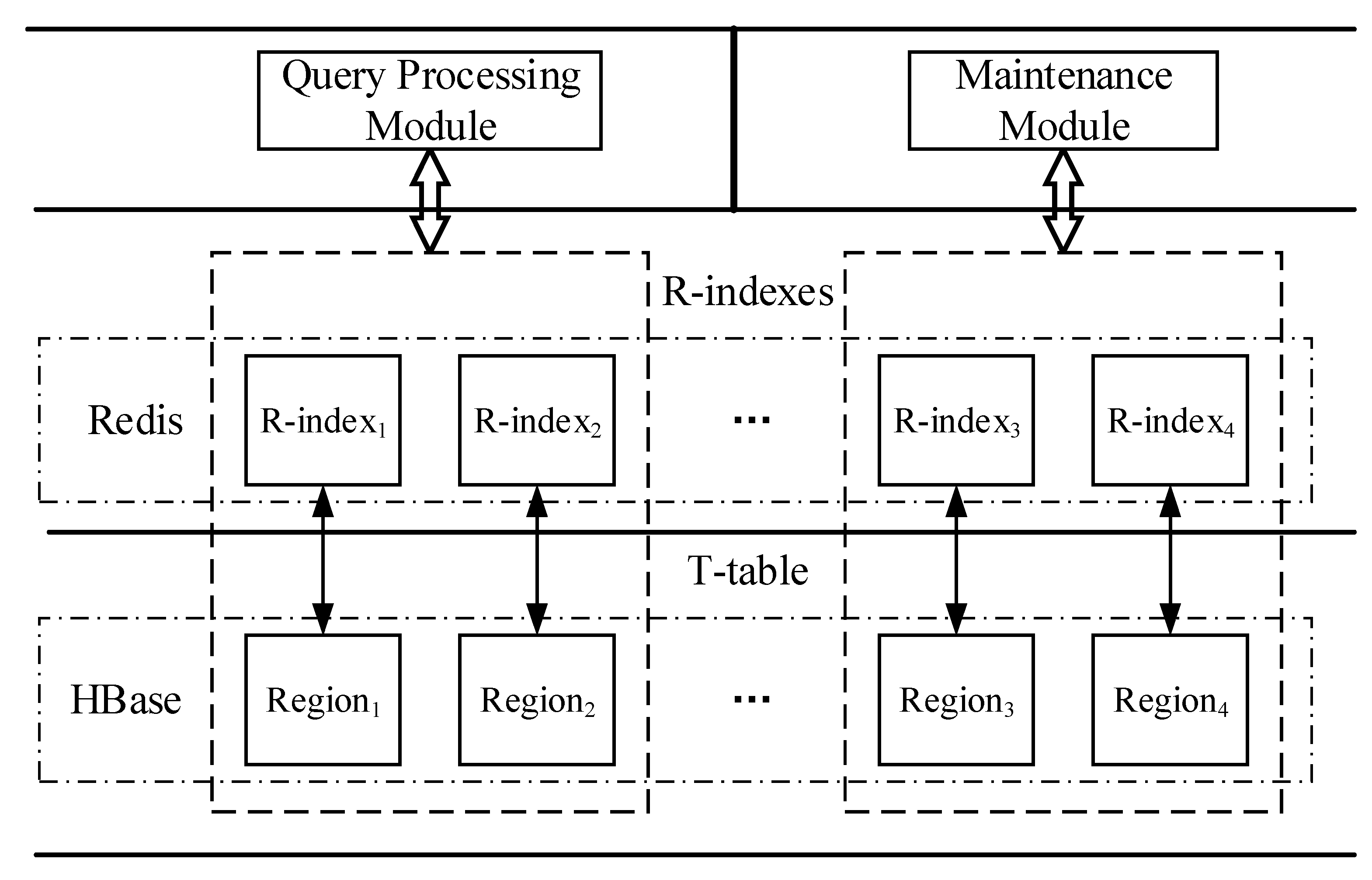
4.1. Overview

Figure 2 gives a full picture of DFTHR. It is composed of four modules:
  • T-table: used to persist storage trajectory data in HBase cluster. It adopts a segment-based data model to organize the trajectory data, and a bulk-based partitioning model to generate Region boundaries and process splits. This module is detail in Section 4.2.
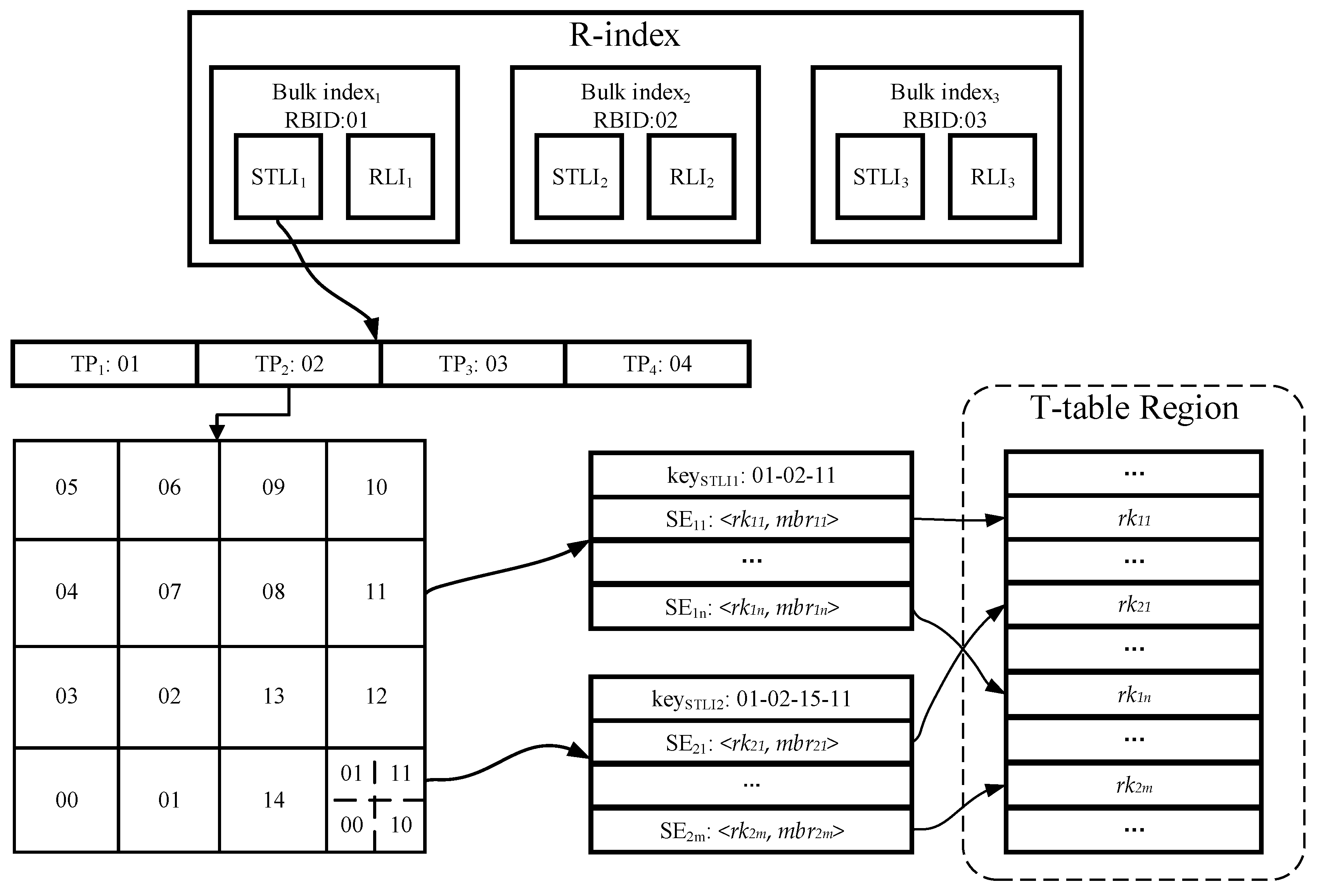
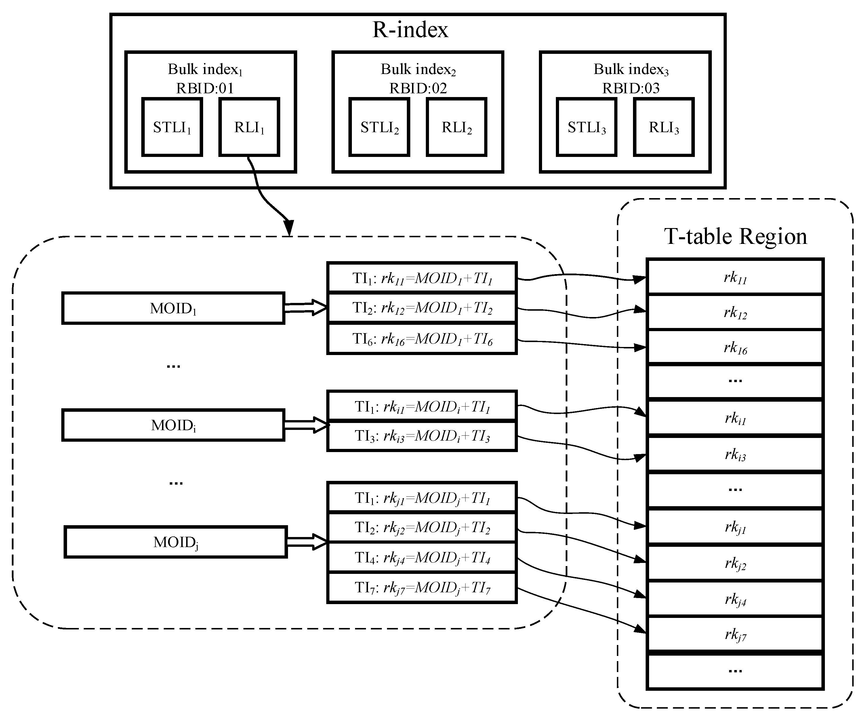
  • R-index: a Region level linear index structure, which stores in Redis so that it is able to process pruning quickly. Each R-index consists of multiple bulk indexes, and each bulk index contains a spatio-temporal linear index (STLI) and a rowkey linear index (RLI); the former is used to process the MBR (minimum bounding rectangle) coverage based pruning, and the latter is used to assist the former to quickly filter out the irrelevant trajectories (detailed in Section 4.3).
  • Query processing module: this implements efficient support for two typical trajectory similarity queries based on trajectory segment based pruning method (described in Section 4.4).
  • Maintenance module: when inserting data, the maintenance module adopts certain strategies to process the split and migration of Regions and indexes. Especially the processing of split, it uses a bulk-based splitting strategy to greatly reduce processing overhead. Maintenance Module ensures the co-location between Region and its corresponding index, thus reducing the communication overhead during query. We give a detailed description in Section 4.5.

4.2. T-Table

In an incremental dataset scenario, we use HBase to organize the trajectory data rather than Spark [25]. This is because: (1) the Spark RDD is read-only. When a new batch of data arrives, Spark needs to spend expensive overhead to repartition all data from scratch and generate new RDDs. While HBase only needs to adjust the size and distribution of some Regions, and the processing overhead is much smaller than Spark, so it can better support incremental updates. (2) As the data scale continues to increase, the memory requirements of Spark will increase. Although Spark can also use the disk to store RDDs, the performance will be greatly reduced. Even when the data scale is large enough, Spark may not be able to complete the whole process due to overflow. Relatively speaking, HBase is more stable.

4.2.1. Trajectory Segment-Based Storage Model

T-table is a HBase table which provides persistent storage support for trajectory data. To better support the Hausdorff distance calculation, we implement T-table based on the following three constraints:
  • Data locality. The trajectory points that belong to the same MO should be assigned to the same Region to avoid the cross-node network overhead for obtaining data of the same MO.
  • Filtering. Since the query results only relate to the trajectory data within the time range, we should avoid storing the whole data of the same MO in a single row, which will increase the filtering overhead of post-processing because the default filtering mechanism of HBase does not take effect until the data is accessed from memory or disk.
  • R-index footprint. The rowkeys of T-table need to be recorded in the entries of R-indexes to implement index function. So the data granularity of the T-table row should not be too small, which may cause huge amount of memory occupation of R-indexes.
Given all this, we design a trajectory segment-based rowkey model, which takes into account the filter and R-index footprint factors so as to avoid containing too much data in each row and effectively control the occupation of R-indexes. In addition, we use MOID as the prefix of rowkey to ensure that the trajectory data of the same MO can be concentrated in the continuous rowkey range, According to Definition 3, the T-table rowkey structure is shown as follows:
r o w k e y = m o i d + t i ,
where moid is the MOID of an MO, and ti is the identifier of a TI. Because the initial digits of MOID usually have a certain distribution pattern, such as the first three characters of the ship identifier (MMSI) representing the country, this is more likely to cause data skew. While the characters at the end of MOID usually have good randomness, so we use the reverse order of MOID in rowkey structure to ensure that the MOID values are randomly distributed in each Region. Similar to the representation of MOID in T-table, MOID also represents in reverse order in R-indexes, maintenance module and query processing module.
In terms of column family and column, because HBase has poor support for multiple column families, one column family called Traj is assigned to store all trajectory points. The column qualifier is represented by the timestamp of trajectory point, location and other information are stored as data cells.
As mentioned earlier, we also build the index with the trajectory segment as the basic element, hence the entire system is implemented based on trajectory segment. Compared to a MO-based data model (storing and indexing data by treating the whole data of the same MO as the basic unit), the trajectory segment based data model has stronger spatio-temporal distinguishing ability, so it has better index pruning power and data filtering effect. On the other hand, compared to a point-based data model (storing and indexing data by treating each trajectory point as an independent element), the trajectory segment data model sacrifices a certain index pruning power and data filtering capability, but it occupies much less memory than the former, and the access efficiency is more efficient, which can be more suitable for massive trajectory data.

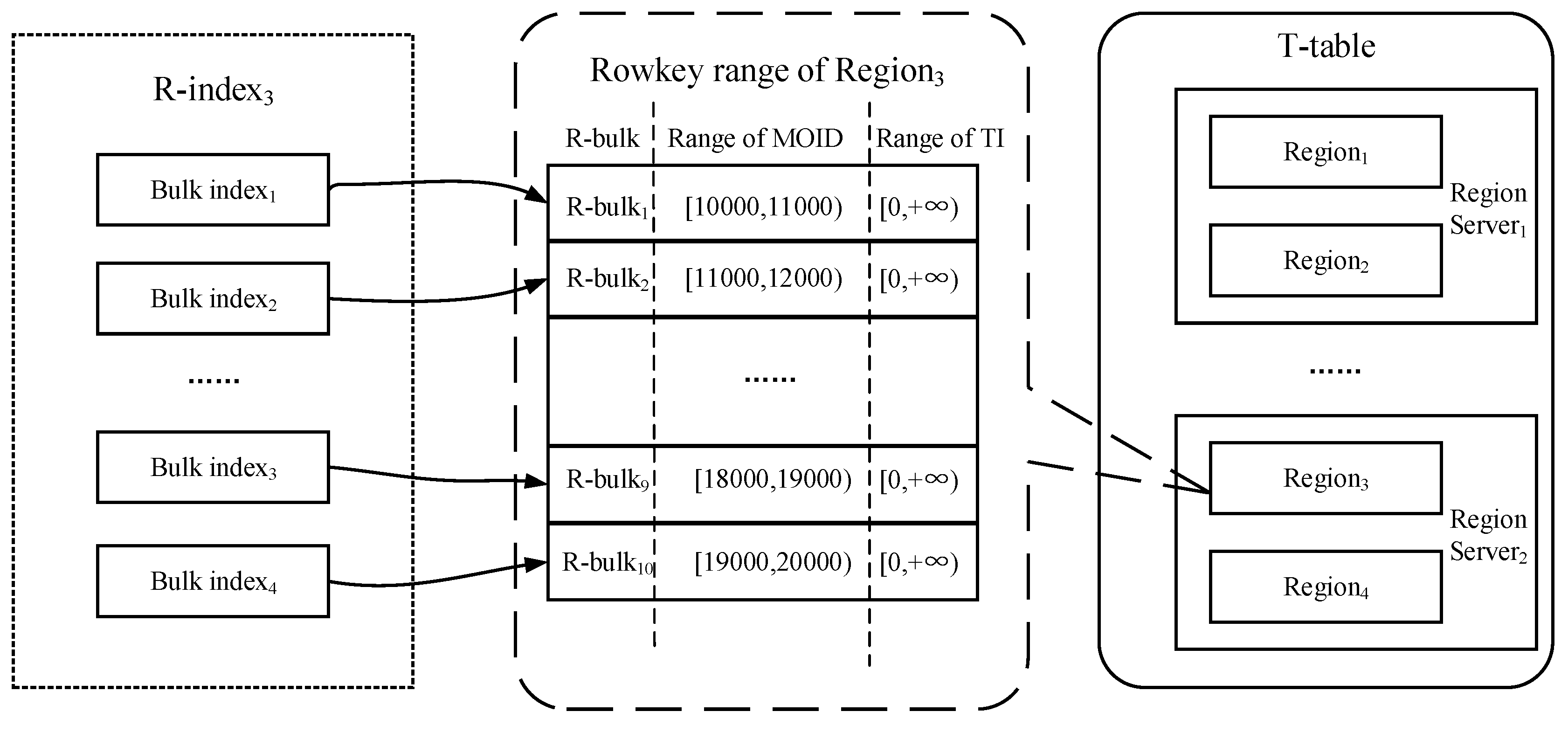
4.2.2. Bulk-Based Partitioning Model

In HBase, data partitioning is achieved by dividing the rowkey range of each Region. Firstly, in order to avoid the distribution of rowkeys of the same MO in different Regions, we can specify the rowkey boundary of each T-table Region by dividing the range of MOID. Secondly, in the case of the incremental dataset, the states of T-table Regions may need to be adjusted to some extent, and we should split or assign some Regions to avoid data skew. Hbase system has a mature mechanism to split or assign Regions, but it cannot maintain the R-index structure that is the local index of each T-table Region. An R-index usually contains hundreds or thousands of index entries, and maintaining it with an efficient strategy helps reduce processing overhead.
Given all this, we instantiate the bulk-based partitioning model. We divide the whole range of MOID into a lot of fine-grained ranges, and several consecutive fine-grained ranges determine the MOID range of a Region. For ease of identification, each fine-grained range is defined as a rowkey bulk (R-bulk), we use the starting MOID of the R-bulk as its identifier (denoted as RBID). For example, the Region with a value range of MOID with [10000, 20000) shown in Figure 3 consists of 10 R-bulks with [10000, 11000), [11000, 12000) … [19000, 20000). Corresponding to the Region structure of T-table, an R-index is also composed of several bulk indexes, and each bulk index corresponds to an R-bulk (R-index structure is detailed in Section 4.3).
Moreover, in the process of data insertion, when the data size of a Region goes above the threshold, this Region and the corresponding R-index need to be split to adjust the load. Profit from the bulk-based partitioning method, we can process it quickly in a bulk-based split approach. If the distribution of the Regions in HBase cluster is skewed, we extend the original load balance strategy of HBase to achieve synchronous assignment of R-indexes. After introducing the R-index structure, we will introduce this split and assignment process in Section 4.5. Certainly, because the R-bulk structure exists only at the logical level and does not affect the physical structure of the Regions, so the bulk-based method only optimizes the processing cost of R-indexes and has little influence on Regions. Overall, it is beneficial to reduce the overhead of adjusting data distribution.
Each RegionServer maintains a BM-table to record the metadata information of all R-bulks on it. BM-table is an Redis Sorted Set structure, and which can be accessed quickly through an user-designated specified key (such as “999999999”). Each data item of BM-table is represented as a tuple <rbid, reid, rsize>, where rbid is the RBID value of an R-bulk, reid is the identifier of a Region to which the current R-bulk belongs, and rsize is the total amount of trajectory data stored in the corresponding R-bulk. The data items in BM-table are organized according to the rbid values, so that the corresponding data items of the R-bulk belonging to the same Region can be gathered together for easy access. When a Region need to be split, the rsize information provided by BM-table will be used to assist in finding the appropriate Region split point (Detailed in Section 4.5). In addition, BM-table is also used to provide a convenient entrance for accessing the R-index entries.

4.3. R-Index

The calculation algorithm of the Hausdorff distance usually improves the efficiency by means of spatial index (such as R-Tree), while we do not consider the spatial attribute in the rowkey structure of T-table, so it is difficult to support the calculation of Hausdorff distance by T-table alone. In order to overcome this problem, we introduce a Region-level index structure named R-index to implement the support for Hausdorff distance calculation. An R-index is a hybrid linear index, which consists of several of bulk indexes. R-index is based on the following four considerations for design and implementation:
  • Access efficiency. The R-index structure does not store actual trajectory point data, so the footprint required is much smaller than the T-table. In order to efficiently access the index data, we implement the deployment of R-indexes through the in-memory database Redis.
  • Pruning. Creating a single index entry for the whole trajectory data of an MO may lead to very limited pruning power, because it may result in a large overlap among index entries. Therefore, R-index is also implemented by indexing the trajectory segment, which helps to reduce the overlapping areas.
  • Network and maintenance overhead. Based on the consideration of reducing network overhead, we should ensure the co-location between each T-table Region and its corresponding R-index. In the incremental data loading scenario, the state of Region may change due to the increase in data, and the corresponding R-index should be kept up to date (such as split or move). Considering that the update and maintenance cost of linear index is much lower than that of R-Tree, and it can be better applied to the key-value store of Redis, so we use a bulk-based hybrid linear index structure to implement R-index. Furthermore, all Redis instances should be deployed in stand-alone mode, namely each RegionServer deploys an independent Redis instance. Compared with the mode of Redis cluster, the stand-alone mode can implement the co-location between any Region with the corresponding R-index without defining some sort of complex sharding strategy.
As mentioned in Section 4.2.2, an R-index consists of several bulk indexes, and each bulk index corresponds to an R-bulk. A bulk index consists of a spatio-temporal linear index (STLI) and a rowkey linear index (RLI). Where STLI is used to index spatial-temporal attributes, while RLI is implemented by indexing rowkeys. To ensure that the trajectory data and its corresponding index data can co-reside on a node, the update of R-index is performed by HBase Observer coprocessor. After the client inserts trajectory data through Put API, the Observer triggers the update of R-index by capturing the post Put event [23].

4.3.1. Spatio-Temporal Linear Index (STLI)

STLI is a spatiotemporal linear index structure, each STLI entry indexes trajectory segments in a certain spatiotemporal range. Unlike the tree index, the linear index does not contain the actual hierarchical structure, and its hierarchical information hides in the key encoding, so designing a reasonable data structure for the key of STLI is the key to ensuring query performance. According to the R-bulk structure, the key structure of STLI is shown as follows:
k e y S T L I = b i c o + t p c o + g r i d c o + c i f c o .
The key of STLI is spliced by four parts: the bulk index code bico, the time period code tpco, the grid cell code gridco and the CIF (Caltech Intermediate Form) quad-tree [26] code cifco. The design of each part is introduced as follows:
  • Bico is the RBID value of the corresponding R-bulk, which is used to identify the bulk index to which the current STLI entry belongs.
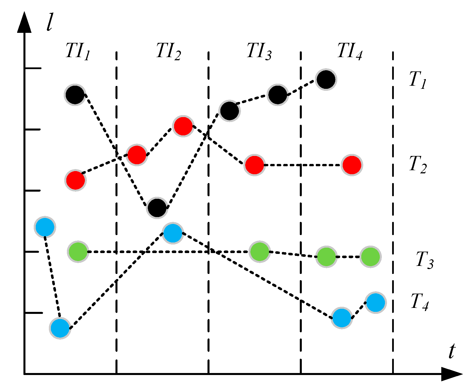
  • In order to index the time attribute, we divide the time dimension into multiple equal-length time periods (TPs) in accordance with time series. Any TI element of trajectory segment must be fully enclosed between the starting and end timestamps of a single TP element to avoid any a trajectory segment being indexed by multiple STLI entries. Since all TPs are of equal length, we can use the starting timestamp as the value of tpco.
  • For indexing the spatial attribute, the whole space is first divided into multiple grid cells of the same size as the initial granularity, and next all the grid cells are encoded through adopting a certain encoding technique (such as Z-ordering, Hilbert curve [27]), and each encoding value is treated as the value of gridco to provide index function. However, the grid structure cannot solve data skew, and some grid cells overlaps with too many MBRs of trajectory segments. For such grid cells, we adopt the CIF quad-tree to further divide them to eliminate data skew. In the process of further division, except that the kind of trajectory segment whose MBR intersects with multiple grid cells is still indexed by the intersecting grid cells, other trajectory segments only are indexed by the minimum quad-tree nodes within a defined depth range which surround their MBRs. With quad-tree encoding, we can obtain a quad-tree code cifco for each CIF quad-tree node. Compared with using CIF quad-tree structure alone, our hybrid index structure which combines grid index with CIF quad-tree can effectively reduce the amount of query processing in the massive data, because there is no node with large coverage area in our index structure. Naturally, this index structure also incurs additional storage overheads due to certain data redundancy.
For each grid cell or CIF quad-tree node, it maps to a Redis Hash, and each index entry of trajectory segment (denote this index entry as SE) is stored in it as a filed-value pair <rk, mbr>, where the field rk is the rowkey of a trajectory segment, and the value mbr is the MBR attribute. The structure of STLI is shown in Figure 4, where the Redis key 01-02-11 and 01-02-15-11 map to a gird cell and a CIF quad-tree node respectively. Organizing SEs with Redis Hash has a following advantages: We can find the specific SE in average O(1) time, avoiding the traversal of the SEs in the set, which helps to quickly process the data update.
Given a time range trq and a spatial range srq, the spatiotemporal query process of each STLI is as below:
According to encoding rules of TP and grid, we can first use trq and srq to obtain a set of tpco values and a set of gridco values respectively. Next, we can quickly obtain the RBIDs of the R-bulks belonging to each Region by dint of a BM-table, and combine the RBIDs with the elements in the two sets to get a list of STLI key prefixes. Then, for each key prefix, we use it to perform a fuzzy query in Ridis to obtain a key set. If the key set contains more than two key elements, this means that the grid cell has a CIF quad-tree sub-structure. So for each key element which maps to a node of CIF quad-tree, we determine whether the corresponding node satisfies the spatial query condition based on its cifco part. In this way, we can obtain a set of candidate keys. Finally, in the Redis Hash corresponding to each candidate key, each SE is pruned based on rk and mbr attributes (through the TI attribute contained in rowkey). After obtaining all the candidate SE elements, we can group them according to MOID to lay the foundation for further processing.

4.3.2. Rowkey Linear Index (RLI)

In the trajectory similarity query, it is necessary to confirm the existence of some trajectory segments. For this, we can confirm by checking whether there are the corresponding rowkeys in the T-table. To avoid the disk I/O overhead caused by checking the existence of rowkeys, we build an in-memory linear index structure RLI for querying rowkeys quickly.
The most intuitive method to implement RLI indexing is directly to use rowkey as the Redis key, but this will result in a lot of data redundancy due to the need to repeatedly record MOID attribute (an MO may contains multiple rows). Based on considerations to reduce space overhead, we organize all the rowkeys of the same MO in a single index entry. In Redis, each index entry corresponds to a Redis Set, where MOID is used as the key, and a TI set which stores the TI parts of rowkeys is used as value. With RLI, we can determine if any rowkey exists in T-table in O(1) time. The structure of RLI is shown in Figure 5.
The query process of RLI is very simple, we first use the MOID to obtain the corresponding index entry, and then query the TI elements within index entry to match TIs. If it is hit, we can conclude that the corresponding rows exist in the T-table. The use of RLI helps to further improve the index-pruning power.

4.4. Query Processing Module

4.4.1. Trajectory Segment-Based Pruning

It is expensive to compute the similarity between two trajectories directly, so according to the data model of the trajectory segment, we propose a lower bound based pruning method and a MBR coverage-based pruning method to reduce the computational cost. Because the k-NN query can also be converted to a threshold-based query by a certain method, so we only need to solve the pruning problem under the threshold-based query scenario.
Applying the branch-and-bound concept to the trajectory similarity query is an effective method, which can first use a certain method of determining the upper bound or lower bound to pruning most of the dissimilar trajectories when accessing the index, thus greatly reducing the computational cost required for distance calculation processing. Therefore, in order to apply the branch-and-bound method to process the similarity query based on the Hausdorff distance, a method for calculating the upper bound or lower bound of Hausdorff distance suitable for the R-index structure is needed. According to literature [28], a lower bound of Hausdorff distance is defined as follows:
Definition 8.
Given two MBRs A and B, a lower bound of the Hausdorff distance from the trajectory points contained in A to the trajectory points contained in B is defined as:
H a u s L B ( A , B ) = max { mindist ( d A , B ) :   d A S i d e s o f ( A ) } ,
where Sidesof(A) is the set of 4 sides of A, and mindist(dA, B) is minimum distance from side dA to B.
However, the lower bound given by Definition 8 is usually applied to the trajectory-based data model, and we need to improve it to be applicable to the segment-based data model.
Given two trajectories Ta and Tq, and let TSSa = {TSa1, …, TSan} denote the set of trajectory segments of Ta, according to Definition 4, the one-sided Hausdorff distance from Ta to Tq can also be expressed as:
h ( T a , T q ) = max { h ( T S a j , T q ) : T S a j T S S a } .
For each h(TSaj, Tq), the lower bound defined by Definition 8 is obviously also stand up, let function M(T) denote the MBR of a trajectory or a trajectory segment, namely h(Taj,Tq)≥ HausLB(M(TSaj),M(Tq)). As a result, for h(Ta, Tq),
h ( T a , T q ) max { H a u s L B ( M ( T S a j ) , M ( T q ) ) : T S a j T S S q } .
Hence, in the threshold-based query, we can easily obtain the following pruning lemma.
Lemma 1.
Given a distance threshold ε, if there exists a trajectory segment T S a j T S S a , such that HausLB(M(TSaj), M(Tq))>ε, then Ta and Tq are necessarily not similar, and Ta should be pruned.
According to the above lemma, we can prune a large number of irrelevant trajectories based on the R-index structure.
However, the calculation cost of the lower bound is relatively expensive. For each calculation of the lower bound, we should calculate the distance between a side and an MBR 4 times. Furthermore, the distance calculation between a side and an MBR is also complex, and we need to first check whether the side is inside the MBR, and then determine whether the two intersect. If either of these conditions is not met, we should find the nearest point on the side to the MBR to calculate the distance. In order to reduce computational complex, a spatial coverage based pruning method is proposed.
According to literature [28], a lower bound of the Hausdorff distance from a trajectory point to an MBR is defined as below:
Definition 9.
Given a trajectory point p and an MBR A, a lower bound of Hausdorff distance from p to the trajectory points confined by A is the nearest distance from p to A, namely,
H a u s L B ( p , A ) = mindist ( p , A ) .
According to Definition 9, it is easy to know that HausLB(p,A) must be smaller than the distance threshold, hence we can use the distance threshold to obtain a spatial range so that the lower bound between any trajectory point contained in it and B satisfies the pruning condition.
Given a query trajectory Td and its MBR M(Tq), we extend the borders of M(Tq) by the distance threshold ε and obtain a new spatial range R(Tq)as shown in Figure 6. For the 4 sides of M(Tq), the trajectory points which satisfy ε are contained in the rectangular areas Me, Mw, Ms and Mn, respectively. For the 4 vertexes of M(Tq), the trajectory points which satisfies ε are contained in the sector areas Mes, Mws, Men and Mwn, respectively. So the lower bounds between all the trajectory points covered by R(Tq) and Td satisfy ε, and we can obtain the spatial range coverage-based pruning lemma.
Lemma 2.
Given two trajectories Ta and Tq, if R(Tq) can’t fully cover all the trajectory points of Ta, then Ta and Tq are not similar, and Ta should be pruned.
However, the R-indexes do not contain the actual trajectory point data, so Lemma 2 is difficult to apply directly. Considering that each trajectory segment in the R-index is indexed in the form of MBR, we can process pruning based on the idea of MBR coverage. For spatial range R(Tq), since the calculation cost of determining the spatial relationship between an MBR and a non-rectangular area is relatively high, we also use an MBR M(R(Tq)) to approximate R(Tq). According to the spatial relationships of the MBRs, we can infer from Lemma 2 to get the MBR coverage-based pruning lemma.
Lemma 3.
Given two trajectories Ta and Tq, if M(R(Tq)) can’t fully cover the MBR of every trajectory segment of Ta, then Ta and Tq are not similar, and Ta should be pruned.
For example, in Figure 6, the MBRs of some trajectory segments of the trajectories T1 and T2 are not fully covered by M(R(Tq)), so T1 and T2 should be pruned.
According to Lemma 3, we can achieve pruning by determining the covering relationship between MBRs. The computational cost of determining whether an MBR is fully covered by another MBR (or rectangular area) is much lower than the cost of computing the lower bound, and it only needs to check whether the coordinates of the lower left corner and the upper right corner of one MBR are in the coordinate range of another MBR (or rectangular area). In contrast, the pruning accuracy based on MBR coverage is lower than that based on the lower bound, such as the trajectory T2 cannot be pruned through the MBR M(R(Tq)), but which can be filtered out through the lower bound value, as shown in Figure 6. So we can first perform the coarse pruning through the MBR coverage-based method, and then do further pruning based on the lower bound between MBRs. In addition, for the MBRs fully covered by M(R(Tq)), we can quickly check whether the lower bound distance between it and R(Tq) is smaller than the distance threshold according to the principle of MBR coverage. Hence, we can filter out some MBRs which do not need to be checked by calculating the lower bound, thus further reducing the computational cost. The process flow is as follow.
For each MBR fully covered by M(R(Tq)), we check whether it is fully covered by the two rectangular areas M e M ( T q ) M w or M s M ( T q ) M n . If it is fully covered, the trajectory points confined by it must satisfy the distance threshold, and the lower bound calculation is not needed. For example, in Figure 6, the MBRs of the trajectories T3 are fully covered by M s M ( T q ) M n , so T3 can be directly considered as a candidate trajectory without calculating the lower bound. If the MBR is not fully covered by the two rectangular areas, and it may overlap with the non-rectangular areas of R(Tq) (namely Mes, Mws, Men and Mwn), the lower bound calculation for it is necessary. This is because we cannot determine whether the trajectory points in a rectangular area are fully covered by a non-rectangular area based on the spatial relationships. For example, in Figure 6, some MBRs of T4 are not fully covered by the sector areas Mwn, but all the trajectory points of T4 are contained in Mwn. For another example that some MBRs of T2 are also not fully covered by the sector areas Mws, but some trajectory points of T2 are out of R(Tq). Thus, we can obtain the following lemma:
Lemma 4.
Given a trajectories Tq and a trajectory segment TSa, if the MBR of TSa is fully covered by either of M e M ( T c ) M w and M s M ( T c ) M n , the lower bound between the MBRs of TSa and M(Tq) must be less than the distance threshold; otherwise, we should calculate the lower bound to determine.

4.4.2. Threshold-Based Query

Because the trajectory similarity queries involve multiple trajectories, to improve query efficiency, we implement a parallel query algorithm based on the HBase endpoint coprocessor. According to the introduction of the T-table and R-index, every T-table Region and its R-index co-reside on the same node, and the data of the same MO is distributed in the same Region. Therefore, when processing a query, each endpoint can handle sub-query independently, without the need to synchronize to other tasks to share data. Moreover, all endpoints are run locally, thus effectively controlling communication overhead and improving execution efficiency.
Given a time range trq, a query trajectory Tq, a distance threshold ε. Algorithm 1 introduces the detailed steps. For each threshold-based query, we can divide it into multiple sub-queries, and each sub-query can be independently processed through the Endpoint on the corresponding T-table Region (line 1 to 13). For each T-table Region, we can obtain the corresponding STLIs stlisq and RLIs rlisq through the BM-table to process the sub-query task (line 2 to 3). After all sub-queries have been executed, we collect the query results on the client and return them to the user (line 14). Here, we mainly introduce the steps of the endpoint-based sub-query:
Algorithm 1 Threshold-Based Query
Input: Query time range trq, Query trajectory Tq, Distance Threshold ε;
Output: A set of Similar Trajectories;
1for each T-table Region do in parallel
2stlisqgetSTLIs();
3rlisqgetRLIs();
4sessstlisq.rangeQuery(M(R(Tq)), trq, ε);
5sessrlisq.removeElementsBySegment(sess, trq);
6sesslowerBoundPruning(sess, ε, Tq);
7sesstwoSidedPruning(sess, ε, Tq);
8  for each sesi in sess do
9   if distFrom(sesi, Tq)≤ε then
9    TCRq.add(Ti);
11   end if
12  end for
13end parallel
14return client.collect(TCRq);
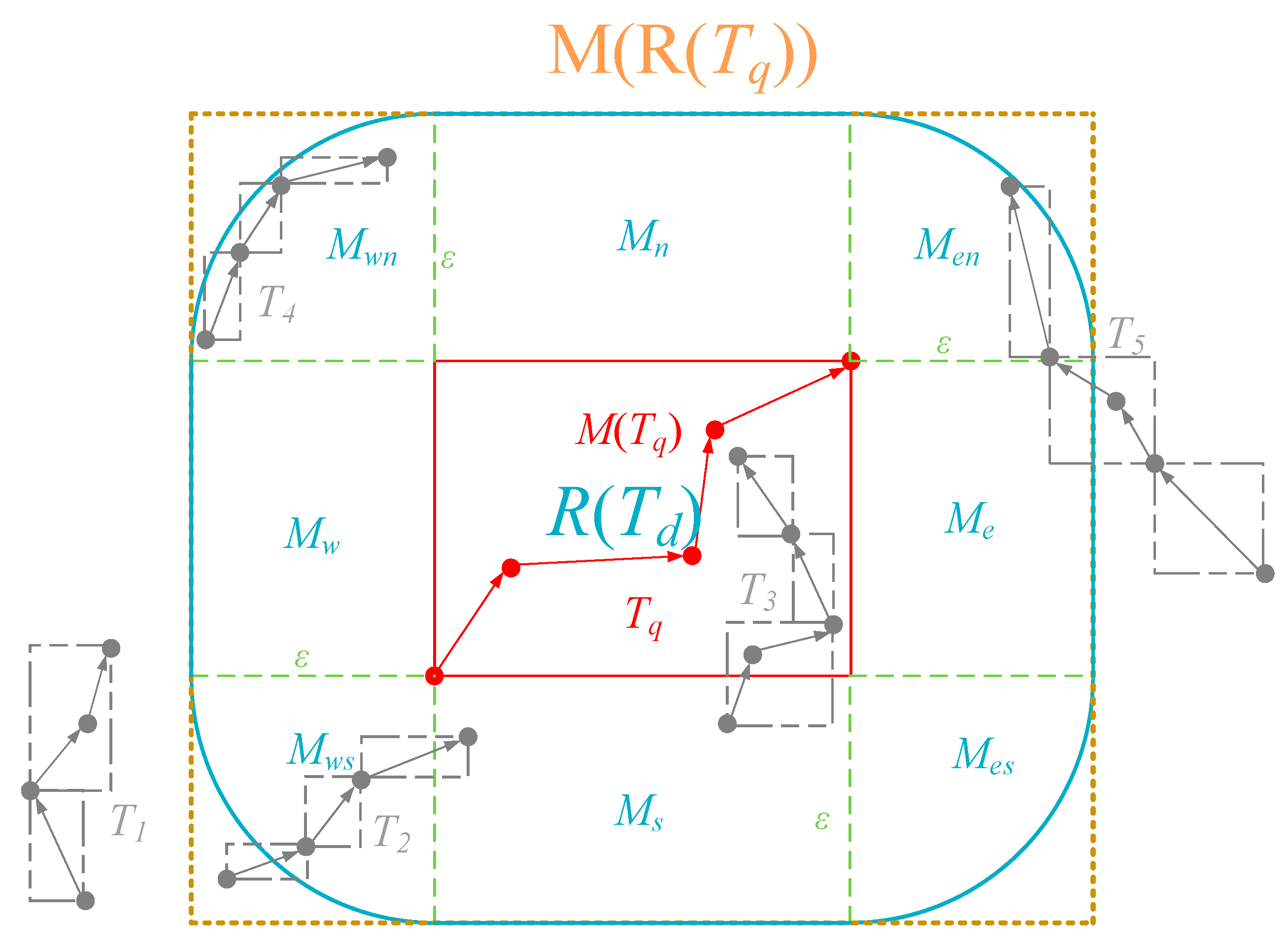
  • MBR coverage based pruning (line 4 to 5). We first obtain an extended MBR M(R(Tq)) according to Tq and ε. Next we invoke a spatiotemporal range query in stli sq by M(R(Tq)) and trq (see Section 4.3.1 for query process in STLI). After getting all the candidate SE elements, we group them according to MOID attribute, and obtain a SE set based on MO grouping sess = {ses1, ses2, …, sesn}, where each sesi = {sei1, …, seim} (1 ≤ in) is a set of candidate SE elements of an MO. In order to facilitate the description, we define this MO corresponding to sesi element as moi, whose MOID is moidi, and the trajectory generated by moi in trq is Ti. However, each query result sesi can only indicate that Ti have some MBRs of trajectory segment that are fully covered by M(R(Tq)), and according to the requirements of Lemma 3, we need to further check whether all the MBRs of Ti are fully covered by M(R(Tq)). For this, we query rlisq by using trq and each moidi to obtain a rowkey set of the trajectory segments rksi. If at least one rowkey that exists in rksi does not exist in the corresponding sesi, this sesi should be removed from sess.
  • Lower bound based pruning (line 6). For each sesi in sess, according to Lemma 4, we first select which SE elements need to further determine the pruning by calculating the lower bound. Next, we calculate the lower bound from each selected SE element to M(Tq), and according to Lemma 1, if there exists a SE element seg = <rkg, mbrg > in sesi, such that HausLB(mbrg, M(Tq))> ε, then we should remove the current sesi from sess.
  • Two-sided based pruning (line 7). Considering that the two-sided Hausdorff distance is used as the distance function of the similarity query, for each sesi in sess, we swap Ti to Tq, and repeat the steps of MBR coverage-based pruning and lower bound-based pruning. If there exists an MBR of a trajectory segment in Tq, such that it does not meet the MBR coverage requirement or the lower bound requirement with Ti, then we should remove the corresponding sesi from sess.
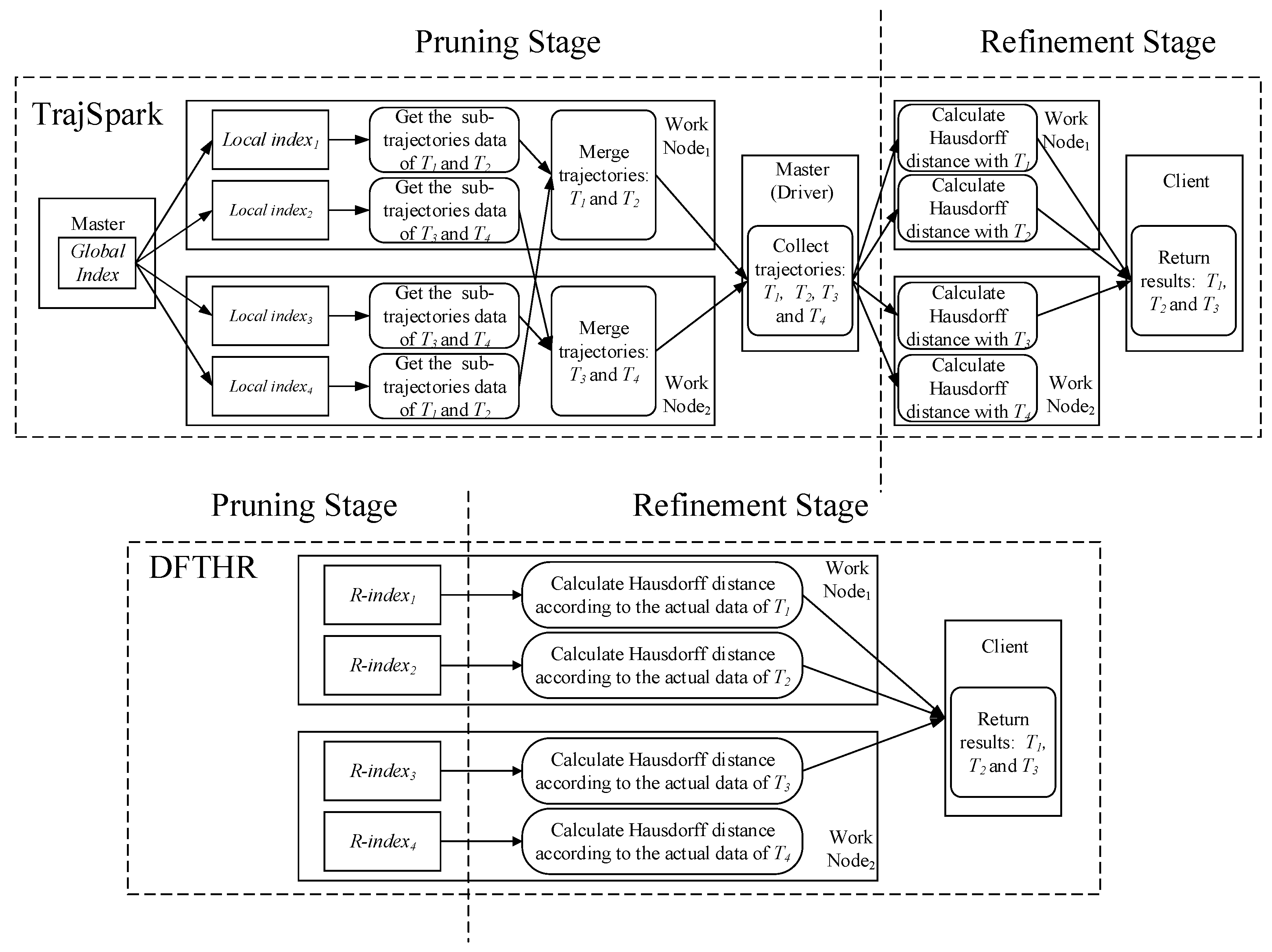
  • Refining (line 8 to 12). For each sesi in sess, we calculate the Hausdorff distance between Ti and Tq, and check whether the distance value is not beyond ε. Finally, we obtain a collection of trajectories TCRq that satisfy ε and return it to the client. In order to calculate the Hausdorff distance, we need to access the T-table Region through the rowkeys contained in sesi to get the actual trajectory data of Ti. In consideration of reducing the disk overhead, we use the INC-HD (incremental Hausdorff distance) algorithm [28] to calculate the distance. This is because this algorithm can filter more trajectory segments by a more efficient upper bound than others, and the data access overhead is smaller.

4.4.3. k-NN Query

For k-NN queries, we can convert them to threshold-based queries and then process them, and the processing flow is shown in Algorithm 2. Given a time range trq, a query trajectory Tq, we first estimate a distance threshold ε according to k in line 1, and send trq, Tq and ε to all T-table Regions. In each T-table Region, the Endpoint performs the subtask of the threshold-based query, in order to enhance the readability, we use function thresholdQuery (trq, Tq, ε) to represent the subtask (line 3 to 5). Next, client collect the query results TCRq of each T-table Region, if the total number is smaller than k, we increase the value of ε and run the threshold-based query repeatedly until the number is not less than k (line 2 to 7). Finally, we choose the k candidate trajectories Tsk as the final results according to the Hausdorff distance and return them to the user from lines 8 to 9.
Algorithm 2 k-NN Query
Input: Trajectory number k, Query time range trq, Query trajectory Tq;
Output: k most similarity trajectories Tsk to Tq;
1εestimateThreshold(k);
2repeat
3  for each T-table Region do in parallel
4   TCRqthresholdQuery (trq, Tq, ε);
5  end parallel
6  εε.increase();
7until client.sum(TCRq.size)≥k
8Tskclient.collect(TCRq).top(k);
9return Tsk;
Incremental iterative: The initial estimated distance threshold may not satisfy that at least k data trajectories are covered, so we may need to adjust the distance threshold and run an iterative process of the threshold-based query. In the iterative process, the selected candidate trajectories do not need to participate in the next iteration, so it can be considered to reduce the computational scale by incremental iterative computation. For that, after completing each iterative process, we cache the MOIDs of all the candidate trajectories in the local Redis for avoiding repeated processing in next iteration. After each MBR coverage pruning processing (detailed in Section 4.4.2), we can quickly filter out the selected elements from sess according to the cached MOIDs, thereby further reducing the computational overhead.

4.5. Maintenance Module

The maintenance module is used to dynamically maintain the data distribution of the whole system, ensuring that the system always performs trajectory similarity query with minimal communication cost. In the incremental dataset scenario, as data scale grow, the distribution of T-table may need to be changes to balance the load of the system, and the load balancing adjustment in HBase is mainly done by splitting and assigning Regions. Since the R-index has to be co-located with each T-table Region, we need to handle the split or assignment of the R-index accordingly when the status of the corresponding T-table Region changes. On the basis of the HBase coprocessor and R-index structure, Maintenance Module can handle the above tasks efficiently, the implementing process is as follows.
For handling Region split, a bulk-based split mechanism is used in preference, namely R-bulk is the basic unit of Region split. The selection of the split point is the core of Region split, we discuss it first. When a Region need to be split, we first obtain the RBID and the data size information of each R-bulk contained in the Region through BM-table, and sort them according to the ascending order of the RBID values, and obtain a sorted set rbss = { <rbid1, rbsize1>, <rbid2, rbsize2> …, <rbidn, rbsizen> }, where rbidi and rbsizei, (1 ≤ in) are the RBID and the data size of the i th R-bulk in the Region, respectively. Next, we pre-split the Region with the starting MOID of each R-bulk (namely RBID) as the pre-split point, and calculate the data size of each new Region respectively after each pre-split. For the above process, we can use rbss to complete it quickly. Let rbidj, (1 ≤ jn) be the pre-split point of pre-split, and the data sizes of the two new Regions rsize1 and rsize2 are computed as below:
{ r s i z e 1 = k = 1 j 1 r b s i z e k r s i z e 2 = m = j n r b s i z e m .
Based on load balancing considerations, the data sizes of the new Regions should be as equal as possible, so we choose the RBID value from rbss as the actual split point which minimizes the difference between rsize1 and rsize2.
Before the HBase system performs a split operation on a Region, the Observer coprocessor captures the preCompleteSplit event to trigger the aforementioned split point selection policy. A rowkey value which is used to split the current Region is constructed by the selected RBID value, and is returned to the HBase system for performing the splitting operation. This rowkey is obtained by adding an all-0 suffix to the selected RBID, it is smaller than all the actual rowkey values of the MO corresponding to the RBID to avoid deploying the data of the same MO to different Regions.
After the Region is split, Observer captures the postCompleteSplit event to trigger the split of the corresponding R-index. At this point, we can modify the data items of the corresponding R-bulk in BM-table to establish the mapping relationship between the corresponding R-indexes of the new Regions and the related bulk indexes. This operation does not need to adjust any bulk index entries, so the processing cost is very low.
The bulk-based splitting mechanism has the following advantages: It ensures that the R-index can be split in O(1) time, so the maintenance cost for index structure is very low, which is suitable for handling incremental data. On the other hand, because the dividing of R-bulks is based on the MO-based approach, our splitting mechanism will ensure that all data of the same MO locate in the same Region after split.
In some extreme cases, most of the data in a T-table Region may be concentrated in very few R-bulks, and the bulk-based splitting strategy does not work well. In this regard, we scan the rows to obtain the data size information of each MO corresponding to these R-bulks, and split each of these into several smaller ones according to the data size information. Then, we split the corresponding bulk indexes, benefit from the linear structure, the split for each bulk index can be done in O(n) time, where n is the number of index entries contained in the bulk index.
When the difference in the number of Regions distributed on different RegionServers is too large, and the HBase system should assign some Regions through load balancing adjustment, Observer triggers the migration of the corresponding R-indexes by capturing the post-Balance event. First, the information of the assigned Regions, source RegionServers and destination RegionServers are obtained by reading the Region Plan parameter. For each assigned Region, since the corresponding R-index is independent, we can directly obtain all the relevant index data from the Redis in the source RegionServer, and then insert it to the Redis of the destination one, which will not affect other Regions or indexes. Finally, we add or delete the related data items in the corresponding M-tables.

5. Experiment

5.1. Set Up

All experiments were conducted in a cluster with 5 nodes, one of which is the master node and the other 4 nodes act as the data nodes. Each node runs Ubuntu 16.04 LTS on 6 cores Intel Xeon E5-2620 V2 CPU, 16 GB memory and 2 TB disk, nodes are connected through a 1 gigabit Ethernet switch. DFTHR is implemented based on Hadoop 2.7.3, HBase 1.3.0, Redis 3.0.
The experiment uses the global AIS data [29] in July 2012 as the dataset. It contains about 1.66 billion messages sent by more than 200,000 ships and is about 200 GB in size. To simulate the incremental data loading scenarios, we split the dataset into multiple batches in the following two methods.
Chronological order-based (CO-based) batches: Considering that new batches of data are appended on a daily, weekly or monthly basis in many real applications, we split the dataset into multiple chronological batches, each of which is about 40 GB.
Random order-based (RO-based) batches: Considering that some datasets in real-life applications are not organized according to a certain order. Hence, we do not consider the spatio-temporal distribution of the trajectory data, and randomly divide the dataset into five batches and each which comprises about 40 GB.
In DFTHR, we set the lengths of TI of trajectory segment and the TP of STLI to 2 h and 24 h respectively, and Initialize the gird size of R-index to 1°. According to the reporting interval of AIS, a single trajectory segment can contain up to 3600 trajectory points. We evaluate the performance of DFTHR with SIMBA [21] and TrajSpark [10] in the fields of scalability and query latency. The scalability is evaluated when each data batch of data is appended, and the query latency is represented by the average response time of several queries.
Here we give a simple example to illustrate the differences among the three schemes. The trajectory points of 4 trajectories T1, T2, T3 and T4 are divided into two batches in chronological order and inserted into a cluster containing two work nodes and one master node, where the trajectory points contained in the time interval TI 1 and TI2 are the first batch, and the trajectory points contained in the time interval TI 3 and TI4 are the other. The results of data distribution are shown in Figure 7, we analyze each scheme one by one.
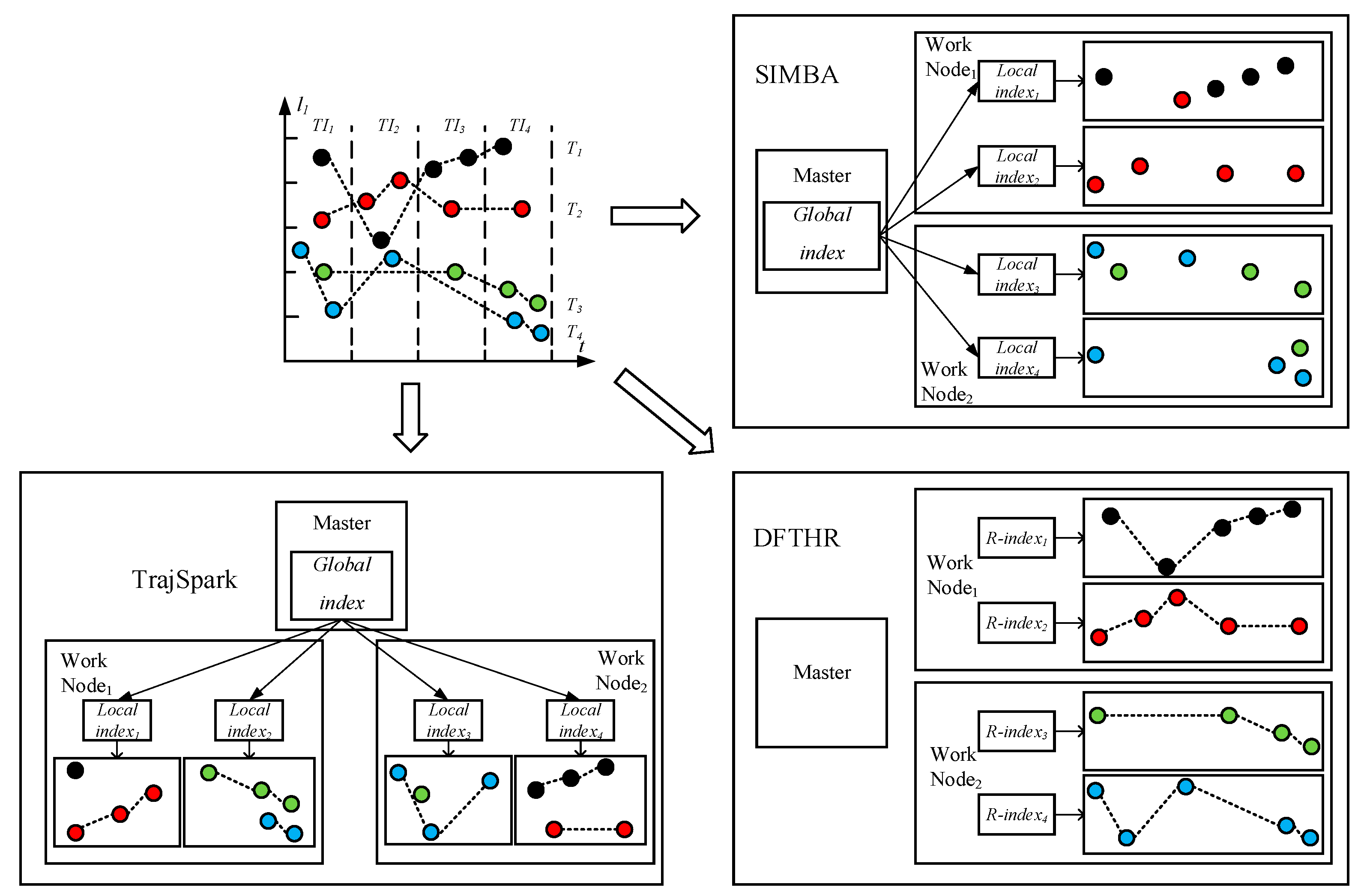
  • SIMBA. SIMBA follows a certain spatio-temporal partitioning strategy to distribute the trajectory data on the partitions of the work nodes, and use trajectory point as the basic data unit. As can be seen from Figure 7, it does not store the data of the same MO on the same node or even the same partition. When each batch of data arrives, it needs to repartition all data. For each data partition, this implements a local index structure to support spatio-temporal queries, and maintains a global index structure on the master node for coarse pruning.
  • TrajSpark. The structure of TrajSpark is similar to SIMBA, which also includes local indexes and global index, and does not organize the data of the same MO on the same node. The differences are that, first, when data batches are inserted in chronological order, TrajSpark can process only the new data without affecting the historical data, as can be seen from Figure 7, and the second batch inserted is distributed in the different partitions from the first batch. Second, the trajectory data is compressed and stored in the partition in the form of a sub-trajectory.
  • DFTHR. The biggest difference between DFTHR and the above two schemes is that it always constrains the data of the same MO to the same partition in the form of trajectory segment. In addition, since it uses HBase instead of Spark, it supports incremental inserting and does not need to adjust all partitions to accommodate data distribution changes. When the state of a partition needs to change, it can alleviate the processing overhead based on the bulk-based maintenance strategy.
Next, we take a threshold-based query as an example to illustrate the query process. Suppose that in this query trajectories T1, T2, T3 and T4 can all be selected as candidates during the pruning phase, and T1, T2 and T3 are selected as the results by refining. Considering that both SIMBA and TrajSpark are based on Spark, the query process is similar. Here we only give a comparison for query process of TrajSpark and DFTHR, as shown in Figure 8.
As can be seen in Figure 8, TrajSpark first performs rough pruning through the global index, and then obtains the candidate sub-trajectories by querying the local indexes in parallel. Next, it performs data shuffling to merge the sub-trajectories into trajectories, and collects all the candidates on the driver node. Finally, TrajSpark initiates parallel processing again to calculate the actual distance value, and returns the results to the client. It can be seen that the entire process involves an amount of cross-node communication. Since DFTHR stores all index data and trajectory data of the same MO on one partition, after obtaining the candidates by pruning, the distance calculation can be directly performed locally, so the inter-worker transmission cost can be avoided.

5.2. Performance of Data Insertion

Firstly, we investigate the performance of data insertion when each of CO-based batch is loaded into these schemes. Figure 9a shows the total running time, a natural observation is that TrajSpark requires less time, and its insert performance is relatively stable; this is because TrajSpark only needs to handle the new loading batch without repartitioning all data in the case of CO-based batches, while DFTHR needs to split and assign some Regions and the corresponding R-indexes during loading. The bulk-based method is used to reduce the processing overhead of R-indexes, but the processing overhead cannot be completely avoided, so DFTHR takes more time than TrajSpark. Otherwise, SIMBA spends the most time because as each batch of data arrives, it needs to repartition all data through a static partitioning strategy named STRPartitioner. Figure 9b presents the data and index footprint of different schemes. Among them, TrajSpark takes up the least space, because it uses a certain compression strategy to compress the trajectory data. SIMBA requires more space overhead than DFTHR since SIMBA organizes trajectory data in the form of point, so it requires a certain amount of storage cost to record the MOID attribute redundantly.
Next, we study the performances of different schemes by using RO-based batches. Figure 9c indicates that DFTHR outperforms TrajSpark and SIMBA significantly, this is because that the optimized partitioning strategy of TrajSpark is not valid for RO-based batches. Like SIMBA, it also needs to repartition all data when each batch arrives. In terms of space overhead (the smaller the better), these schemes perform slightly worse on RO-based batches than CO-based one as shown in Figure 9d, since a larger number of index entries should be created.

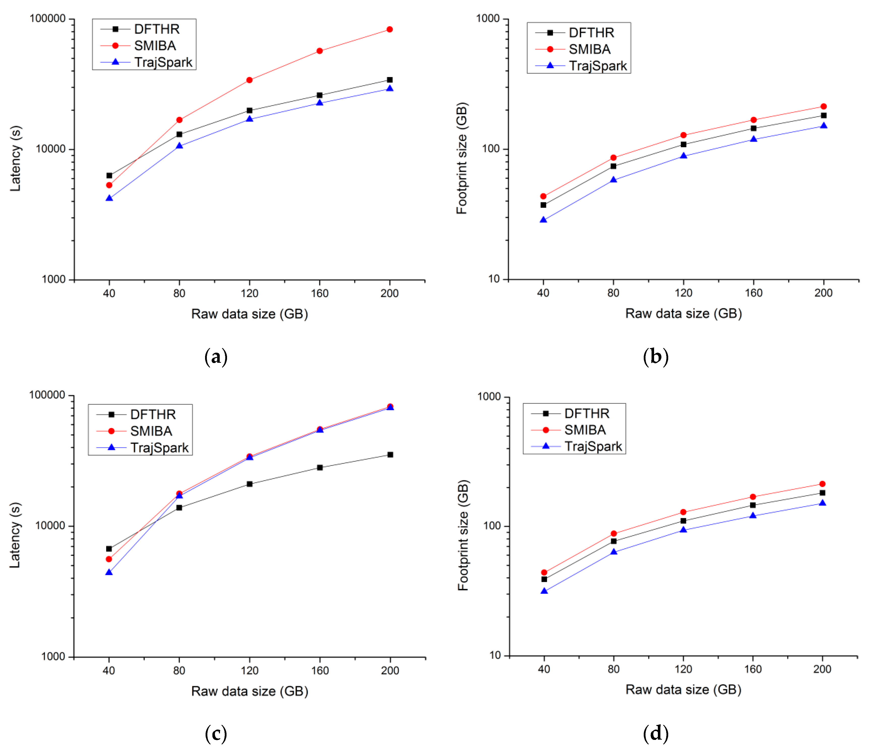
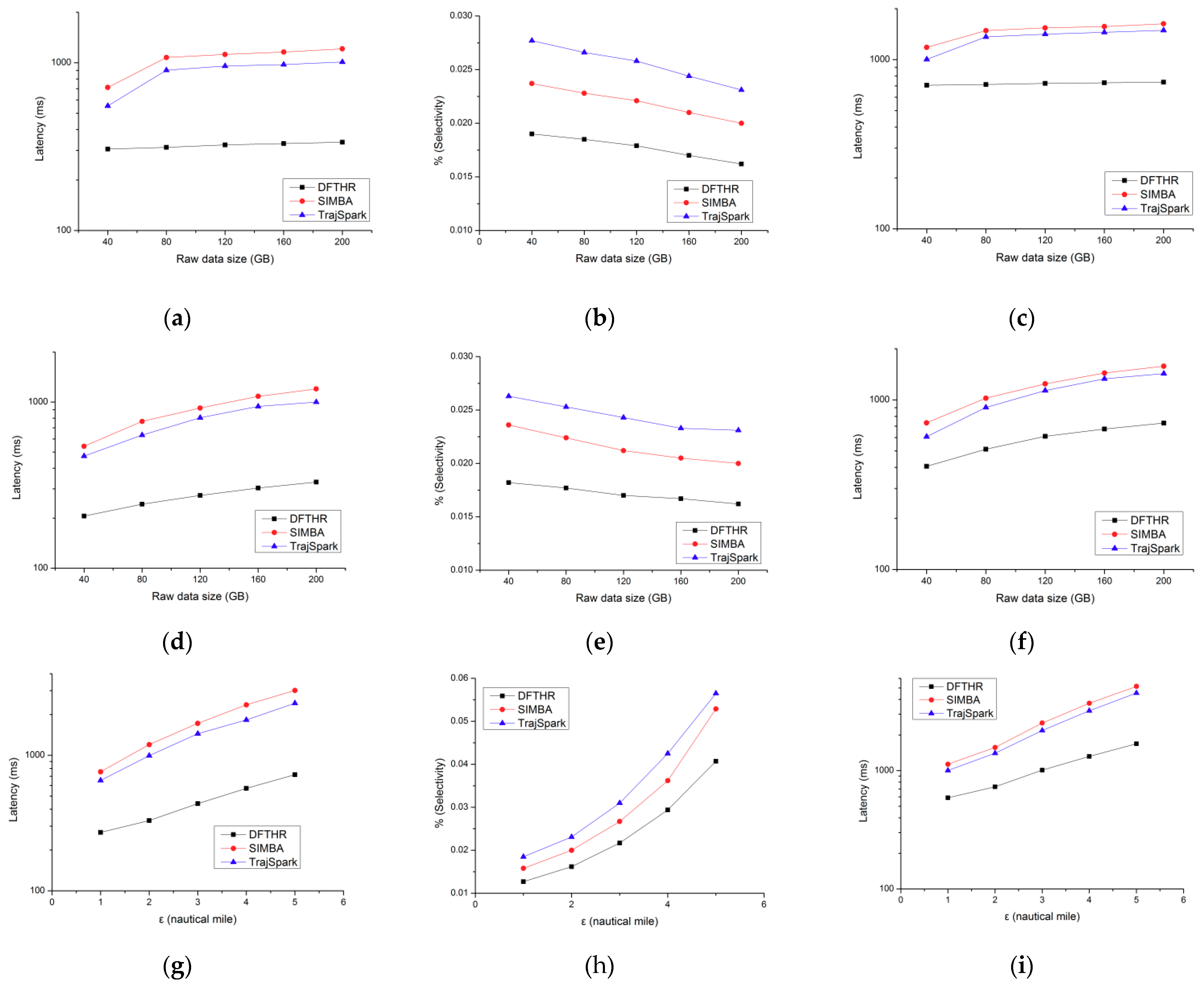
5.3. Performance of Threshold-Based Query

In terms of query performance, we first examine the efficiency of threshold-based query under different data scales. We evaluate the three aspects of pruning latency, selectivity (The ratio of the number of candidates after pruning to the total number of MOs) and query latency. We randomly select 10 trajectories as query reference, and set the distance threshold and the query time range to 2 nautical miles and 24 h respectively. Figure 10a,c displays the results of average pruning latency and query latency in the case of CO-based batches respectively. We can see that all three behave relatively steady, this is because they can filter out the irrelevant data by utilizing the time condition. Since most RDD data of TrajSpark and SIMBA can be stored in memory in the case of 40 GB, consequently, the pruning latency and query latency are significantly smaller than other data scales. For selectivity, as shown in Figure 10b, three schemes show a similar trend and become more selective as the data size grows. Figure 10d,f shows that the pruning latency and the query latency of the three schemes increases linearly with the increase of RO-based data scale. This is because the data density increases as the data scale increases in the case of RO-based data batches, and the amount of data that need to be processed is also in growth. Similarly, the value of the selectivity is decreasing due to the growth of the number of MOs.
In addition, we also conduct experiments on these schemes under various distance thresholds. Experiments are performed under the condition of 200 GB, and distance threshold varies from 1 nautical miles to 5 nautical miles. The results are shown in Figure 10g–i, as the distance threshold increases, the pruning latency and query latency also increase due to the large increase in the number of candidate trajectories. As the number of candidates increases due to the increase of the query range, the selectivity values of the three schemes all show an increasing trend.
Among the three schemes, DFTHR has the highest pruning and query performance in different conditions for the following reasons: (1) all the index entries and trajectory data of the same MO co-reside on same node, and the shuffling step is not needed to merge the index data or trajectory data of the same MO, so the inter-worker transmission cost can be avoided; (2) the segment-based data model and pruning method have a higher pruning precision, and can filter out a larger number of irrelevant trajectories. Moreover, the use of the rowkey index structure RLI further improves the pruning efficiency. Therefore, DFTHR has the best selectivity.

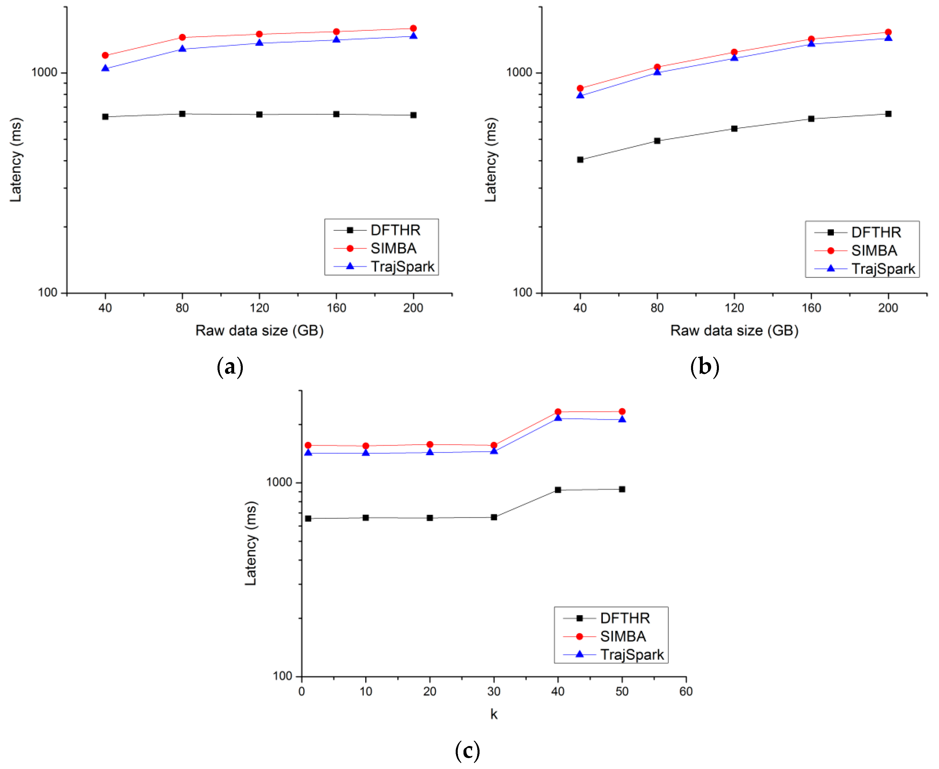
5.4. Performance of k-NN Query

In the k-NN query experiment, we select the trajectories generated by 10 ships within 24 as the query reference, and set the value of k to 10. Figure 11a,b show that DFTHR outperforms SIMBA and TrajSpark under both the CO-based batches and the RO-based batches, in addition to the reasons mentioned in Section 5.3, the incremental iteration strategy adopted by DFTHR also help to reduce the processing overhead.
Next, we test the impact of different k values on queries. The data scale is 200 GB, and the query reference is still the 10 trajectories sampled in 24 h. As shown in Figure 11c, in a certain value range of k, the query performance of these scheme is not affected by the varying of k because the candidate trajectories selected when k = 1 already contains a sufficient number of trajectories to cover a sufficiently large k value. When the k value is large enough, the distance threshold required to complete the query further increases, resulting in a longer query delay.

6. Conclusions

In the paper, we propose DFTHR, a distributed framework for trajectory similarity query based on HBase and Redis. DFTHR provides the trajectory similarity threshold-based query and k-NN query according to the Hausdorff distance. It utilizes a trajectory segment-based data model with a number of optimizations for storing, indexing and pruning to organize and process trajectory data efficiently. Furthermore, DFTHR adopt a bulk-based partitioning model and certain optimization strategies to alleviate the cost for splitting partitions, so that the incremental dataset can be supported efficiently. Additionally, DFTHR introduces a co-location based distributed strategy and a node-locality-based parallel query algorithm to reduce the inter-worker cost overhead. We validate the data appending and query performance of DFTHR by experiments on real dataset. Experimental result show that DFTHR outperforms existing schemes. In future, we plan to support more distance functions, such as DTW, LCSS, etc.

Author Contributions

Conceptualization, J.Q. and Q.L.; Data curation, J.Q.; Methodology, J.Q.; Supervision, L.M.; Validation, J.Q. and Q.L.; Writing—original draft, J.Q.; Writing—review and editing, L.M. and Q.L. All authors have read and approved the final manuscript.

Funding

This research was funded by National Natural Science Foundation of China, grant number 61802425.

Conflicts of Interest

The authors declare no conflict of interest.

References

  1. Salmon, L.; Ray, C. Design principles of a stream-based framework for mobility analysis. GeoInformatica 2017, 21, 237–261. [Google Scholar] [CrossRef]
  2. He, Z.; Ma, X. Distributed Indexing Method for Timeline Similarity Query. Algorithms 2018, 11, 41. [Google Scholar] [CrossRef]
  3. Morse, M.D.; Patel, J.M. An efficient and accurate method for evaluating time series similarity. In Proceedings of the 2007 ACM SIGMOD International Conference on Management of Data, Beijing, China, 11–14 June 2007. [Google Scholar]
  4. Bai, Y.B.; Yong, J.H.; Liu, C.Y.; Liu, X.M.; Meng, Y. Polyline approach for approximating Hausdorff distance between planar free-form curves. Comput. Aided Des. 2011, 43, 687–698. [Google Scholar] [CrossRef]
  5. Zhou, M.; Wong, M.H. Boundary-Based Lower-Bound Functions for Dynamic Time Warping and Their Indexing. In Proceedings of the 2007 IEEE 23rd International Conference on Data Engineering, Istanbul, Turkey, 15–20 April 2007. [Google Scholar]
  6. Zhu, Y.; Shasha, D. Warping indexes with envelope transforms for query by humming. In Proceedings of the 2003 ACM SIGMOD International Conference on Management of Data, San Diego, CA, USA, 9–12 June 2003. [Google Scholar]
  7. Ranu, S.; Deepak, P.; Telang, A.D.; Deshpande, P.; Raghavan, S. Indexing and matching trajectories under inconsistent sampling rates. In Proceedings of the 2015 IEEE 31st International Conference on Data Engineering (ICDE), Seoul, Korea, 13–17 April 2015. [Google Scholar]
  8. Zheng, B.; Wang, H.; Zheng, K.; Su, H.; Liu, K.; Shang, S. SharkDB: An in-memory column oriented storage for trajectory analysis. WWW 2018, 21, 455–485. [Google Scholar] [CrossRef]
  9. Peixoto, D.A.; Hung, N.Q.V. Scalable and Fast Top-k Most Similar Trajectories Search Using MapReduce In-Memory. In Proceedings of the Australasian Database Conference, Sydney, Australia, 28–30 September 2016. [Google Scholar]
  10. Zhang, Z.; Jin, C.; Mao, J.; Yang, X.; Zhou, A. TrajSpark: A Scalable and Efficient In-Memory Management System for Big Trajectory Data. In Proceedings of the Asia-Pacific Web (APWeb) and Web-Age Information Management (WAIM) Joint Conference on Web and Big Data, Beijing, China, 7–9 July 2017. [Google Scholar]
  11. Xie, D.; Li, F.; Phillips, J.M. Distributed trajectory similarity search. Proc. VLDB Endow. 2017, 10, 1478–1489. [Google Scholar] [CrossRef]
  12. Shang, Z.; Li, G.; Bao, Z. DITA: A Distributed In-Memory Trajectory Analytics System. In Proceedings of the 2018 International Conference on Management of Data, Houston, TX, USA, 10–15 June 2018. [Google Scholar]
  13. Alt, H.; Scharf, L. Computing the hausdorff distance between curved objects. JCG Appl. 2008, 18, 307–320. [Google Scholar] [CrossRef]
  14. Apache HBase. Available online: https://hbase.apache.org/ (accessed on 8 January 2019).
  15. Redis. Available online: https://redis.io/ (accessed on 8 January 2019).
  16. Alt, H.; Godau, M. Computing the Fréchet distance between two polygonal curves. IJCGA 1995, 5, 75–91. [Google Scholar] [CrossRef]
  17. Müller, M. Information Retrieval for Music and Motion; Springer: Berlin/Heidelberg, Germany, 2007; pp. 69–84. [Google Scholar]
  18. Yang, K.; Shahabi, C. A PCA-based similarity measure for multivariate time series. In Proceedings of the 2nd ACM International Workshop on Multimedia Databases, Washington, DC, USA, 13 November 2004. [Google Scholar]
  19. Vlachos, M.; Kollios, G.; Gunopulos, D. Discovering similar multidimensional trajectories. In Data Engineering, 2002. In Proceedings of the 18th International Conference, San Jose, CA, USA, 26 February–1 March 2002. [Google Scholar]
  20. Chen, L.; Özsu, M.T.; Oria, V. Robust and fast similarity search for moving object trajectories. In Proceedings of the 2005 ACM SIGMOD International Conference on Management of Data, New York, NY, USA, 14–16 June 2005. [Google Scholar]
  21. Xie, D.; Li, F.; Yao, B.; Zhou, L.; Guo, M. Simba: Efficient in-memory spatial analytics. In Proceedings of the 2016 International Conference on Management of Data, San Francisco, CA, USA, 26 June–1 July 2016. [Google Scholar]
  22. Vora, M.N. Hadoop-HBase for large-scale data. In Proceedings of the 2011 International Conference on Computer Science and Network Technology (ICCSNT), Harbin, China, 24–26 December 2011. [Google Scholar]
  23. Vashishtha, H.; Stroulia, E. Enhancing query support in hbase via an extended coprocessors framework. In Proceedings of the European Conference on a Service-Based Internet, Poznan, Poland, 26–28 October 2011. [Google Scholar]
  24. Han, J.; Haihong, E.; Le, G.; Du, J. Survey on NoSQL database. In Proceedings of the 2011 6th International Conference, Pervasive Computing and Applications (ICPCA), Port Elizabeth, South Africa, 26–28 October 2011. [Google Scholar]
  25. Zaharia, M.; Chowdhury, M.; Franklin, M.J.; Shenker, S.; Stoica, I. Spark: Cluster computing with working sets. In Proceedings of the Usenix Conference on Hot Topics in Cloud Computing, Boston, MA, USA, 22–25 June 2010. [Google Scholar]
  26. Samet, H. The quadtree and related hierarchical data structures. CSUR 1984, 16, 187–260. [Google Scholar] [CrossRef]
  27. Lawder, J.K.; King, P.J.H. Querying multi-dimensional data indexed using the Hilbert space-filling curve. SIGMOD 2001, 30, 19–24. [Google Scholar] [CrossRef]
  28. Nutanong, S.; Jacox, E.H.; Samet, H. An Incremental Hausdorff Distance Calculation Algorithm. Proc. VLDB Endow. 2011, 4, 506–517. [Google Scholar] [CrossRef]
  29. Harati-Mokhtari, A.; Wall, A.; Brooks, P.; Wang, J. Automatic Identification System (AIS): Data reliability and human error implications. J. Navig. 2007, 60, 373–389. [Google Scholar] [CrossRef]
Figure 1. Examples of trajectories and trajectory segments.
Information 10 00077 g001
Figure 2. Distributed framework based on HBase and Redis (DFTHR) architecture.
Information 10 00077 g002
Figure 3. T-table and R-index structure.
Information 10 00077 g003
Figure 4. Spatio-temporal linear index (STLI) structure.
Information 10 00077 g004
Figure 5. Rowkey linear index (RLI) structure.
Information 10 00077 g005
Figure 6. Pruning trajectories with distance threshold ε.
Information 10 00077 g006
Figure 7. Example of data insertion.
Information 10 00077 g007
Figure 8. Comparison of query process.
Information 10 00077 g008
Figure 9. Time and storage cost for inserting data: (a) time cost of chronological order (CO)-based batches, (b) space cost of CO-based batches, (c) time cost of random order (RO)-based batches, (d) space cost of RO-based batches.
Information 10 00077 g009
Figure 10. Performance of threshold-based query: (a) pruning latency of CO-based batches, (b) selectivity of CO-based batches, (c) query latency of CO-based batches, (d) pruning latency of RO-based batches, (e) selectivity of RO-based batches, (f) query latency of RO-based batches, (g) pruning latency of changing distance threshold, (h) selectivity of changing distance threshold, (i) query latency of changing distance threshold.
Information 10 00077 g010
Figure 11. Performance of k-NN query: (a) result of CO-based batches, (b) result of RO-based batches, (c) result of changing k.
Information 10 00077 g011

