Dynamic Top-K Interesting Subgraph Query on Large-Scale Labeled Graphs

Abstract

A labeled graph is a special structure with node identification capability, which is often used in information networks, biological networks, and other fields. The subgraph query is widely used as an important means of graph data analysis. As the size of the labeled graph increases and changes dynamically, users tend to focus on the high-match results that are of interest to them, and they want to take advantage of the relationship and number of results to get the results of the query quickly. For this reason, we consider the individual needs of users and propose a dynamic Top-K interesting subgraph query. This method establishes a novel graph topology feature index (GTSF index) including a node topology feature index (NTF index) and an edge feature index (EF index), which can effectively prune and filter the invalid nodes and edges that do not meet the restricted condition. The multi-factor candidate set filtering strategy is proposed based on the GTSF index, which can be further pruned to obtain fewer candidate sets. Then, we propose a dynamic Top-K interesting subgraph query method based on the idea of the sliding window to realize the dynamic modification of the matching results of the subgraph in the dynamic evolution of the label graph, to ensure real-time and accurate results of the query. In addition, considering the factors, such as frequent Input/Output (I/O) and network communication overheads, the optimization mechanism of the graph changes and an incremental maintenance strategy for the index are proposed to reduce the huge cost of redundant operation and global updates. The experimental results show that the proposed method can effectively deal with a dynamic Top-K interesting subgraph query on a large-scale labeled graph, at the same time the optimization mechanism of graph changes and the incremental maintenance strategy of the index can effectively reduce the maintenance overheads.

1. Introduction

In the real world, entity-centric applications are constantly increasing, and the study of the interrelationship between entities becomes more and more important. Researchers use graphs to denote the complex relationship among entities and analyze the structural features of graphs, which can extract hidden information from the graphs to solve practical problems. The entity relationship networks consisting of multi-type entities are called heterogeneous information networks, such as the biological information network [1], social network [2], military network and protein-to-protein network, etc., which is abstracted to labeled graphs in this paper.

The subgraph query is the basic problem of graph data processing, namely, to search all matching subgraphs that are isomorphic to the query graph in the data graph. With the rapid development of information technology and the explosive growth of the data [3], more and more studies have focused on the subgraph query of graphs [4,5,6,7,8] to extract the information of interest to the users. However, in practical applications, users are often interested in parts of matching results and hope that by increasing restrictions they can reduce the negative impact of information overload. So, the subgraph query is combined with the Top-k query to solve the problem. Existing Top-K subgraph query methods [9,10] are mainly concentrated on small scale or static graphs, which cannot be directly applied to large-scale dynamic graphs with low query efficiency, high storage costs, etc. In addition, the kind of query is of great significance in practical applications. Taking the authors’ cooperative relationship network of DataBase systems and Logic Programming (DBLP) as an example, the strong K teams with a specific structure where the authors’ work is queried closely together is modeled as an interesting subgraph query problem where user personalization is limited [11]. However, the continuous query based on this application is rarely studied.

Answering such subgraph queries efficiently involves four main challenges: (1) Existing Top-K interesting subgraph query methods are mainly aimed at unweighted query graphs. However, the weights of edges can usually represent a certain relationship between entities, such as the familiarity of two entities, the success rate of completing tasks together, and so on. So, the matching efficiency is extremely low for the queries where user personalization is limited. These are represented as weighted query graphs. (2) We know that the index can speed up the query, but as the size of the data graph increases, consideration should be given to how to further balance the memory overhead, index construction time, and the speed of subgraph query. These constraints should be studied by researchers. (3) Inappropriate matching order can affect matching efficiency. The existing methods are less concerned with the matching order of weighted graphs, which greatly influences the efficiency of the subgraph query on weighted graphs. (4) In practical work, networks change dynamically with time [12], and so the topological structure and properties of graphs will change. In this paper, the research will focus on the problem of the interesting subgraph query on large-scale dynamic graphs. The results of the subgraph query can be dynamically updated, which can obtain the latest and relatively accurate matching results in a time efficient manner.

To address the above problems, we propose a novel dynamic Top-K interesting subgraph query (DISQtop-k for short) method with unique characteristics of nodes and edges based on the sliding window technology [13,14]. Considering some factors, such as the frequent Input/Output(I/O) and network communication overheads, the optimization mechanism of graph changes and the incremental maintenance strategy of indexes are proposed, which reduces the huge overheads caused by redundant operations and the global update. In this paper, the main contributions are as follows:

• A graph topology structure feature index (GTSF index) is proposed. It consists of a node topology feature index (NTF index) and an edge feature index (EF index), which uses the topology structure of nodes and the edge feature information to prune and filter invalid nodes, to obtain a relatively small set of candidate node sets and candidate edge sets.
• A multi-factor candidate set filtering strategy based on the GTSF is proposed, and this strategy is used to further prune the candidate set of the query graph to avoid redundant computation in the matching-validation phase.
• We propose a dynamic Top-K interesting subgraph query method based on the sliding window. First, in the matching-verification phase, a query matching order setting method is given to improve the matching-verification efficiency. Then because dynamic changes in the graph may influence matching results, we divide the matching process into two phase: initial matching and dynamic modified. In the initial matching phase, the initial result set is achieved by matching one by one the candidate set according to the matching order; in the dynamic modified phase, the initial result set is dynamically updated by using the dynamic change of the graph as far as possible to ensure that the real-time and accuracy of query results.
• Taking into account some factors, such as the frequent I/O and network communication, we propose an incremental dynamic maintenance strategy for indexes. As there may be some relationship among the various types of graph change operations in the update interval, the optimization mechanism of graph changes is proposed. By using optimized change operations, indexes are made by local updates to avoid the huge overheads caused by global updates.

At present, most of the subgraph query methods adopt the filtering-validation. According to the different filtering modes, we can classify them into three types: unindexed structures, frequent subgraph indexes, and reachability index filtering.

Unindexed structure approaches will be matched and validated directly. Ullmann [15] is a kind of subgraph isomorphism testing method based on the state space search. It employs the refinement procedure to eliminate successor nodes in the tree search, to achieve the aim of pruning and improve the efficiency of the determining isomorphism. Because of the use of the recursive exhaustive method, it is only applicable to small-scale graphs. VF2 [16] is optimized for Ullmann, and the search space is pruned by using a set of feasibility rules, which increases the order of matching of the query nodes. The VF2 algorithm does not take advantage of index structure or the optimization strategy so that its complexity is super linear. Thus, the query efficiency is extremely low on a large-scale graph. STwig [17] also does not use graphical indexes but uses parallel technology to solve subgraph queries. However, time-consuming join operations and unevenly distributed graph data become the bottleneck of the parallel technology, so that the space complexity and time complexity of STwig are relatively high. TurboISO [18] proposes merging similar nodes (with the same label and located at the same region) in the query graph and transforms the query graph into a spanning tree, filtering out the unfeasible candidate nodes by the path filtering method. BoostIso [19] is optimized for TurboISO. It first merges the similar nodes in the data graph, and then further reduces the unnecessary intermediate results by the path filtering method. However, TurboISO and BoostIso apply only to a query graph and data graph that have similar nodes so it is difficult to apply to a query graph and data graph which does not meet this special requirement. In addition, the runtime of the path filtering method can increase exponentially with the increase in the length of the path. Literature [20] presents a new framework to eliminate the redundant problem of the Cartesian product of non-similar nodes by performing the Core Forest Leaf (CFL) decomposition. At the same time, an auxiliary data structure (Compact Path Index, CPI) is proposed. It can not only be used to calculate the matching order but can also realize data graph pruning. Thus, the possible query results in the data graph can be compressed and encoded.

The frequent subgraph index approach is to find frequent subgraphs or frequently queried subgraphs, and index these frequent structures to avoid excessive joins during the matching process. SUBDUE [21] is the most well-known algorithm for mining frequent subgraphs on a single graph. SpiderMine [22] is optimized for SUBDUE to be used to mine the Top-K maximum frequent patterns from the graph. The above two subgraph query methods only apply to data graphs with frequent subgraph structures.

The reachability index approach constructs index structure and some optimization strategies to cut the candidate set and enumerate the solution gradually and verify the candidate set corresponding to query graph nodes based on backtracking, to recursively form the final query results. Both SPath [23] and GraphQL [24] filter by neighbors of each node to minimize the number of candidate nodes. GraphQL uses the form of breadth-first traversal to further filter candidate nodes, to iteratively search. SPath implements the filtering of nodes by recording some basic paths. Because too much information is recorded in the filtering process, there is an increase in unnecessary memory overheads. Neither of these methods involves repeated enumeration of equivalent nodes and matching sequence selection.

In practical application, users tend to pay attention to the query result of higher interestingness scores, thus, leading to more targeted Top-K subgraph query problems. Due to the particular semantics of the Top-K [25,26,27,28,29,30], the Top-K subgraph query is mainly divided into two parts: The first is to find all the matching subgraphs in the data graph according to the query graph; the second is to rank all the matching subgraphs according to their interestingness score and obtain the K interesting subgraph with the greatest interestingness score. At present, the Top-K subgraph query is mainly divided into two modes: ranking-after-matching mode and ranking-while-matching mode.

The ranking-after-matching mode obtains all the matching subgraphs first, and then sorts these matching subgraphs according to their interestingness score, to get the optimal K matching subgraphs, such as the RAM algorithm. RAM filters candidate sets by establishing the SPath index structure. Then all matching subgraphs are obtained through matching and validation, all the matching subgraphs are ranked according to their interestingness score, to get the optimal K matching subgraphs. Because the process of obtaining all the matching results is relatively complicated, the Top-K subgraph query on a large-scale is less efficient. Ranking-while-matching mode filters out the matching subgraph with a significantly smaller interestingness score in the process of matching and validation, such as the RWM algorithm. To improve RAM, RWM adopts ranking-while-matching mode and proposes two index structures to prune candidate sets. The query efficiency of RAM is relatively high. However, due to the random order of Top-K matching, a large quantity of redundant computation is generated.

Therefore, based on the above analysis, we can see that there are two problems in most of Top-K subgraph query algorithms. First, most algorithms only solve the matching problem of the unweighted query graph and do not consider the user’s personalized requirement; that is, they do not involve the matching process of the weighted query graph. Second, in practical application, the topological structure of the graph changes with time and actual application semantics, but the Top-K subgraph queries of the dynamic graph are relatively few.

The rest of the paper is organized as follows: In Section 2, we explain the basic concepts of this paper, and define the dynamic Top-K approximate query problem. Section 3 and Section 4 detail the proposed index construction and the dynamic query processing method based on the index, meanwhile we give corresponding examples. In Section 5, we present the dynamic optimization maintenance strategy for the proposed index. Extensive experimental analyses are given in Section 6. And the conclusions are given in Section 7.

2. Preliminaries

This section presents the basic concepts and problem description used in this paper.

● Graph label

We focus on the undirected weighted labeled graph as shown in Figure 1, which can be represented as a tuple (V, E, T, L (V), W). Each node denotes an entity in some network, and V is the set of nodes. Edges denote the relationship of nodes and E is the set of edges. T is a set of node types. and L (V) is the label value of node V, which is used to represent some characteristics of the node (entity). Edge weights represent interestingness between nodes and W is the set of edge weights. In Figure 1, taking the authors’ cooperative relationship network of the DBLP as an example, it contains three types of entities that of the author, research field, and journal. Graph labels A, F, J represent different types of nodes and edges and show the relationship among the three types. The edge weights are used to express the degree of cooperation between authors, some author’s published rates in some journals or the similarity between research fields, and so on.

● Interesting subgraph

In reality, according to different query requirements, people tend to be interested in queries that have some kind of structure and hope a more accurate query can be achieved by limiting the special relationship between some nodes in the query graph. For example, in the military network, we need to organize a team of four people to complete a task, which requires that two people have accurate marksmanship, one person is good at English and computers, one person is only good at English, and the two people with accurate marksmanship have worked together many times. That is, the problem of the query can be abstracted as querying a subgraph that has the above structure and whose weights between the nodes have certain limits. This kind of subgraph is usually called an interesting subgraph. This paper will further study the problem of the interesting subgraph query.

● Dynamic Top-K approximate query

The interesting subgraph query will search all subgraphs from the data graph that have the same structure with the query graph and in which the edge weights will satisfy some query restriction. In practice, the association degree among entities is often identified by the edge weight in the labeled graph. We define the association degree as an interesting score. The normalization is defined as follows:

Definition 1.

Interesting Score. If M is a matching subgraph of query graph Q in the data graph G, the matching subgraph M of the interesting score is shown in Formula (1):

$$INT(M)={\displaystyle \sum _{i=1}^{\left|E_M\right|}W(e_i)}$$

(1)

W(e_i) represents the weight of the ith edge in the matching subgraph M.

As shown in Figure 2. P₁ and P₂ are two pairs of matching subgraphs of query graph Q. Their interesting scores are I NT (P₁) = 2.3 and I NT (P₂) =2.1, respectively.

With the further development of information technology, the size of graph data is increasing, and the Top-K query is widely used because it can effectively solve the huge cost of information overload. The Top-K interesting subgraph query on a large-scale graph is modeled as a subgraph search problem with the K greatest interesting score, which is isomorphic to query graph. In practice, however, the topological structure of a network changes with the time and actual application semantics, namely nodes or edges are inserted or deleted in data graph, and how to ensure the high effectiveness of the Top-K interesting subgraph query on the large-scale dynamic graphs will face a severe challenge. The study found that the existing dynamic graph data processing often adopts regular cumulative updates instead of the real-time updates to reduce the huge communication overheads caused by frequent I/O, but it may lead to a certain error in the query result within the update interval. However, the dynamic change of the graph is a long and stable process [31], and the amount of changes over a period of time is much less than the size of the graph. This, in turn, has a relatively small impact on the results of the subgraph query. Therefore, this paper will study the Top-K interesting subgraph approximate query on large-scale dynamic graphs.

3. GTSF Index Construction

The subgraph isomorphism matching is an Non-deterministic Polynomial-complete problem. We know that indexes can speed up the query. But as the size of the data graph increases, how to balance the memory overhead, index construction time, and the speed of subgraph query is a problem that should be considered and further studied by researchers. In general, the search efficiency of algorithms will decrease when the sizes of the data graph and query grow. Most of the existing methods adopt the filtering-validation strategy to establish indexes with filtering capability by extracting the information of the graph nodes or some substructure information, to improve the query efficiency. In this paper, according to the characteristics of the large-scale dynamic labeled graph and making full use of the information on nodes and edges, we propose the novel GTSF index, including the NTF index and the EF index. The NTF index can be used to filter invalid nodes based on the information of node degree, adjacency node and so on, so as to obtain a relatively small set of candidate nodes. The EF index can be used to quickly filter the invalid edge that does not meet the weight-restriction by the type label and weight of the edge, and then obtain a relatively small set of candidate edges.

3.1. NTF Index

The properties of node degree, label type, and different types of adjacency nodes are both iconic and distinguishability in the labeled graphs. Therefore, this paper proposes a novel NTF index based on these features. It consists of two level structures. The top-level structure is indexed according to the type of label node; the bottom-level structure establishes the node topology relationship that each label type contains, to achieve efficient filtering of invalid nodes.

The top-level index item of the NTF is composed of the <node label type, the number of nodes belonging to the type>; the bottom-level index item is composed of the <node id, node degree, and the number of adjacency nodes for each type>. We use the breadth first algorithm to calculate the properties of the label type, degree, adjacency node type and number. Greater node degree provides more and more valuable information in the process of query and matching. Therefore, in this paper, the index items are listed in descending order by node degree. Taking the example of Figure 1, the data graph G contains nodes of type A, F, and J. And its NTF index is shown in Figure 3.

3.2. EF Index

We find that besides the nodes, edges also contain a lot of information, such as edge type, weight, etc., by analyzing the characteristics of labeled graphs. To further filter the invalid structure, we proposed another index that is the EF index. It also contains two level index structures. The top-level structure is indexed according to the edge label type (consisting of two node types); the bottom-level structure contains edge information for each edge label type. The label type and weight of each edge can be obtained quickly by the EF index.

The top-level index item of the EF index is composed of <edge type>, and the bottom-level index is composed of < edge endpoint 1’s id, edge endpoint 2’s id, weight >. The Top-K interesting subgraph query is to query the K highest interestingness score of matching subgraph in data graph G according to query graph Q, and it is known from the definition of interestingness score that it increases with the increase of the edge weight. In this paper, the EF index is listed in descending order to effectively filter edges that do not meet conditions. Still taking the example of Figure 1, the data graph G contains the edges of five types, which are AA, AF, AJ, JF, and FF, and its EF index is shown in Figure 4.

4. Dynamic Top-K Interesting Subgraph Approximate Query based on The Sliding Window

4.1. Multi-Factor Candidate Set Filtering Based on GTSF Index

The processing procedure of Top-K subgraph query is mainly composed of index construction, candidate set filtering, and subgraph matching-verification. By using an efficient graph index and the filtering strategy to filter out elements that clearly violate the query requirements, a relatively small candidate set can be obtained, which can improve the efficiency of the subgraph matching-verification. Therefore, according to the NTF index and the EF index, this paper presents, respectively, the candidate node set filtering strategy (CNFiltering) and the candidate edge set filtering strategy (CEFiltering), to realize the pruning filtering of nodes and edges.

4.1.1. Multi-factor Candidate Node Set Filtering

On a large-scale dynamic graph, users often make a personalized query by limiting some edge weights. So, nodes in the query graph can be divided into special nodes (endpoints of the weighted edge are called special nodes) and common nodes. In the selection of candidate nodes, this paper proposes the CNFiltering strategy considering the limits of node type, degree, the number of adjacency nodes and the edge weight limit. It is illustrated in Algorithm 1.

● Special node filtering (SNF)

The edges based on special nodes must satisfy the limits of weights in the query graph. Therefore, according to the weighted edge type, it will prune edges that do not meet the limits, and screen out the special node candidate set.

● Degree filtering (DF)

Because the degree of each node is not less than the query node in the candidate set, invalid nodes are pruned by using the NTF index, according to the type and degree of the query node.

● Adjacent node label frequency filtering (ANLFF)

The candidate nodes should not only meet the requirements of degree but at the same time the number of each type adjacent nodes should not be less than the number of query node. Therefore, on the basis of DF, we use the NTF index to prune nodes that do not meet the frequency of each type of adjacency nodes, thereby gaining the candidate node set.

Algorithm 1 CNFiltering algorithm

Input:node topology feature index TG, edge feature index EG, node topology feature index TQ, edge feature index EQ

Output:the candidate node set CN 1 CN=NULL; 2 for(traverse e in EQ) do /* Obtain the candidate node set CN of the query graph Q */ 3  if (w(e)!=0) /* Filter special nodes */ 4  CN←SNF (EG,e,CN); 5  CN←DF(TG,e,CN); 6  CN←ANLFF(TG,e,CN); 7  else /* Filter common nodes */ 8  CN←DF(TG,e,CN); 9  CN←ANLFF(TG,e,CN); 10 end for 11 Output C;

In Algorithm 1, the time complexity of Candidate Node Set Filtering is O (n). The main loop operation is in row 4, 5, 6, 8, 9. It takes O (n) time to processes iteratively each node in these rows, where n is the number of nodes in the NTF index. Therefore, the time complexity of Algorithm 1 is O (n). The space complexity is O (n+m) that is because both the NTF index and EF index store each node and each edge only once.

Taking Figure 2 as an example, only the edge (v₁, v₃) of the AJ in Q has a weight of 0.5, so v₁ and v₃ are special nodes. If we retrieve the EF index, we can get the edges of the AJ type that are not less than 0.5; they are (5, 1):0.9, (14, 9):0.7, (10, 9):0.6, (15, 9):0.6 and (14, 19):0.5. Then, according to DF and ANLFF filtering, we can get the candidate set of v₁ and v₃ that are, respectively, {5, 14, 10, 15} and {1, 9, 19}. Common nodes only use DF and ANLFF filtering to get the candidate node set. Finally, we get the candidate nodes CN of Q, as shown in Figure 5.

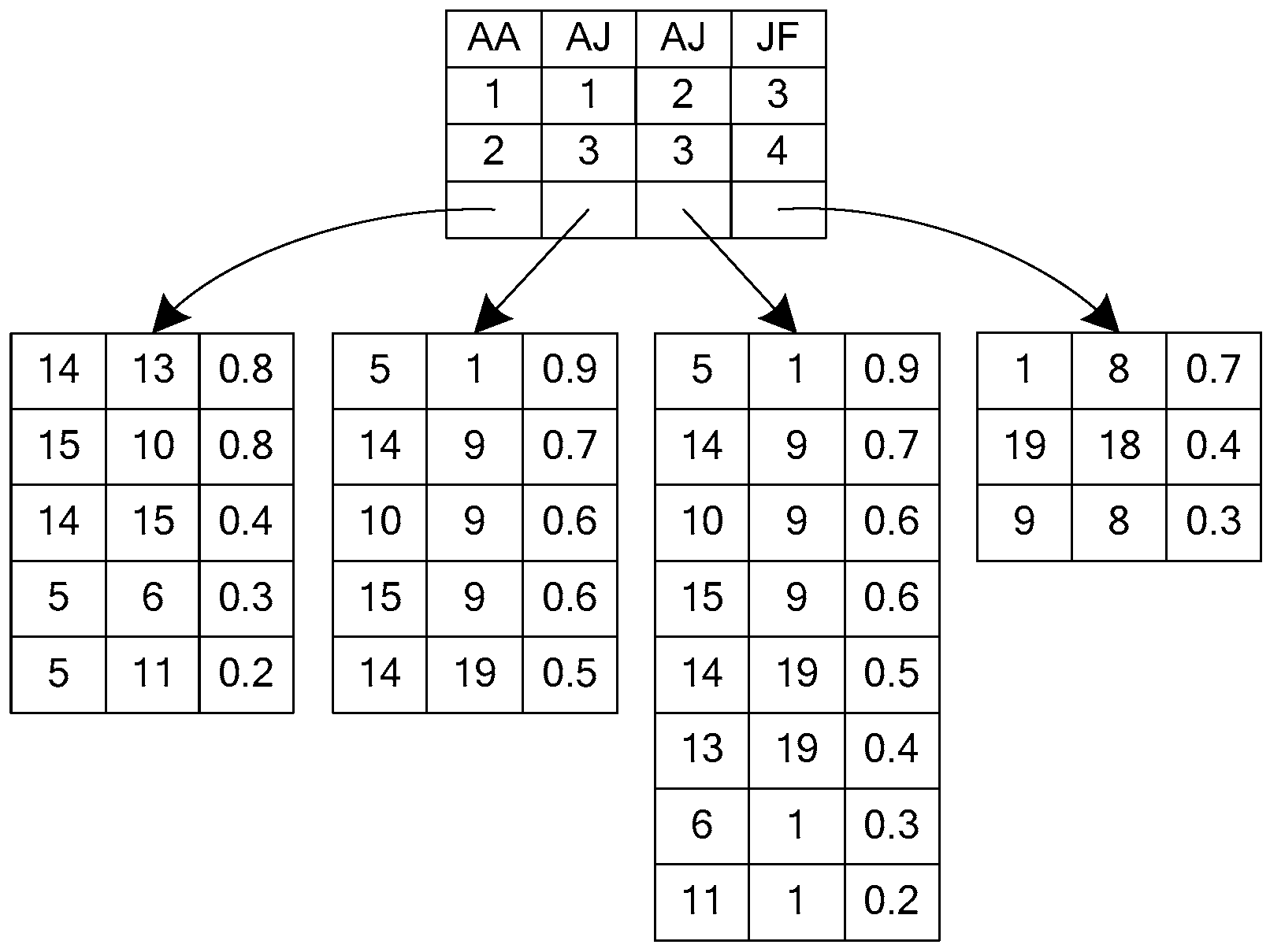
4.1.2. Candidate Edge Set Filtering

The CNFiltering strategy can be used to prune nodes that do not meet requirements effectively, thereby we can obtain a relatively small candidate set of nodes. On the basis of it, we utilize the EF index to mine the information contained in nodes and edges, and propose the candidate edge set filtering strategy, namely CEFiltering. It implements a second pruning of the query graph candidate set, to obtain a better candidate edge set used for final subgraph matching-verification. As shown in Algorithm 2.

● Special edge filtering

In the query graph, we call the edge with weight the special edge. We retrieve the EF index for each special edge to screen edges, whose type is the same as the special edges and weights are not less than the special edges’. The results are called candidate edges. Then, we judge whether two endpoints of each candidate edge are in the corresponding candidate node set. If they exist, the candidate edge is valid, else it is invalid. Finally, we get the candidate set of special edges.

● Common edge filtering

In the query graph, the edge without weight is called the common edge. The filtering of the common edges simply obtains by retrieving the NTF index. To find the same type of edges and the two endpoints of each edge they should be in the corresponding candidate node set. Finally, we get the candidate set of the common edges.

Algorithm 2 CEFiltering algorithm

Input:edge feature index EG, edge feature index EQ, the candidate node set CN

Output :the candidate edge set CE 1 CE=NULL; 2 for(traverse e in EQ) do /* Filter out invalid edges in the query graph Q by using the EF index and candidate node set CN */ 3  for (traverse in CN[e]) do 4   if (w( )<w(e)) 5    return false; 6   else 7    (v, u)←e′; 8   if (v CN || u CN) 9    return false; 10   else 11    return true; 12 output CE;

The main loop operation is rows 2 to 11. It takes O (m) time to visit iteratively each edge, where m is the number of edges in the EF index. Moreover, when an edge is traversed, the candidate node set of the edge endpoints needs to be traversed. It takes O (n′), where n′ is the number of candidate nodes of that visited edge and n′<<n. Therefore, the time complexity of Algorithm 2 is O (nm).

For example, in Figure 2, there are three types of edge, AA, AJ, and JF, in the query graph. Only the edge (v₁, v₃) of the AJ type in Q has a weight of 0.5. According to the EF index, it is found that the edges of the AJ type whose weight is not less than 0.5 have (5, 1):0.9, (14, 9):0.7, (10, 9):0.6, (15, 9):0.6 and (14, 19):0.5. Because the endpoints of the above five edges are all in the candidate node set CN, the candidate set of the edge (v₁, v₃) is {(5, 1):0.9, (14, 9):0.7, (10, 9):0.6, (15, 9):0.6, (14, 19):0.5}. The edge (v₃, v₄) of the JF type in Q is the common edge. Retrieving the EF index, the edge of the JF type can be found, including (1, 8), (19, 18), (9, 8), (2, 8), and (20, 16). The endpoints of (2, 8) and (20, 16) are not included in the corresponding candidate set of v₃ and v₄, so (2, 8) and (20, 16) are invalid edges. The candidate edge set of (v₃, v₄) with filtered out invalid edges is {(1, 8), (19, 18), (9, 8)}. Similarly, candidate edge sets of other common edges can be obtained. The candidate edge set CE of the query graph Q is shown in Figure 6.

4.2. Dynamic Top-K Interesting Subgraph Query

The way of the cumulative update method may result in some errors of the query results during the update interval. So, continuous query results for a period of time may be more analytical than a single result at a certain time. We propose a dynamic Top-K interesting subgraph approximate query method based on the sliding window (DISQtop-K). This method supports the continuous query, which can return continuous results in the query time period for the user. At the same time, for queries during the update interval, we make full use of the graph changes within the time threshold to update the candidate set in time, to ensure the accuracy of the query maximally.

4.2.1. Sliding Window

The sliding window is an important technology to realize the continuous query [32]. It can be divided into two categories: the sliding window based on the number of tuples and the sliding window based on timestamp [33]. The sliding window based on the number of tuples stores the recent arrival of the N tuples, and the window size is fixed; the sliding window based on timestamp stores the tuples that came within T time recently, and the window size is variable. In this paper, the sliding window based on timestamp is used to process the continuous query, to realize dynamic the Top-K interesting subgraph query. The sliding window size is set to T_w = nΔt = {t₁, t₂, …, t_n} (n is a positive integer) and the query interval is set to T_m = mΔt = {t₁, t₂, …, t_m} (m is a positive integer), where Δt is the jump time of the sliding window. Δt and T_w are appointed by the system, and T_m is appointed by the user.

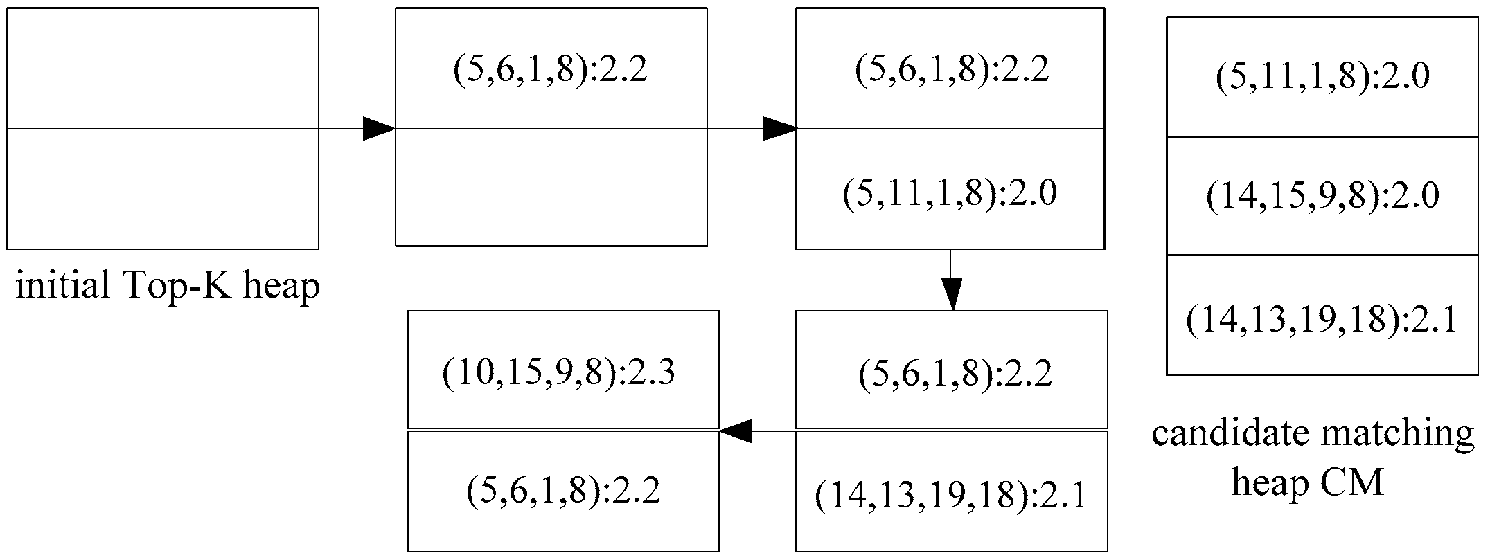
4.2.2. Top-K Interesting Subgraph Matching-validation

The dynamic changes of the graph may have an impact on the matching result of the Top-K interesting subgraph matching-verification. So, the matching process is divided into two phases: initial matching and dynamic modified. In addition, the research of existing Top-K interesting subgraph query algorithms based on the filtering-verification model is found that the matching-verification edge by edge is often adopted in the subgraph matching-verification stage, so the order of verification will affect the query efficiency. We present a query graph matching order setting method.

● Setting query graph matching order

Because the matching-verification adopts the method of matching edge by edge, the edge in the least candidate edge set is used as the initial matching edge, which can effectively reduce iterative times and further reduce unnecessary computational overheads. We know the larger degree of the node, the easier it is to prune invalid nodes in the data graph. In addition, the number of nodes in the data graph which have the same label type with the nodes in query graph is fewer, and they are easier to prune. Therefore, for a node v, we define the Information as the ratio of v’s degree and the number of nodes with v’s type. Information of the edge in the query graph is shown in Formula (2).

$$INF(v_i,v_j)=(\frac{d(v_i)}{f(G,T(v_i))}+\frac{d(v_j)}{f(G,T(v_j))})/2$$

(2)

INF(v_i, v_j) represents Information on any edge (v_i, v_j) of the query graph Q where d(v_i) and d (v_j) represent the degrees of v_i and v_j. And f (G, T (v_i)) and f (G, T (v_j)) represent the number of nodes in the data graph whose label types are same as v_i and v_j. For example, Information of the edge (v₁, v₃) in the query graph Q is INF(v₁,v₃) = (2/9+3/6)/2, whose value is 13/36.

In this paper, we use Information to set the grade of edges in the query graph, and determine the matching order by using the initial matching edge. Information of each edge is calculated by Formula (2). The larger its value, the higher the corresponding edge grade. Starting from the initial matching edge, Information of other edges composed of endpoints of the current matching edge is calculated one by one based on the breadth first method. The edge of the largest Information is selected as the next matching edge, and then the matching order of the query graph is determined iteratively.

● Initial matching-verification

The initial matching will be performed based on the candidate edge set CE. First, the Size-c candidate matching and its upper bound value US (Size-c) are defined.

Definition 2.

Size-c Candidate Matching. Size-c candidate matching represents a partial growth matching when the c edges of the query graph are instantiated in the process of subgraph matching. Its interesting score is the sum of weights of the instantiated edges where c ∈ (1, n) and n is the number of edges in the query graph.

Definition 3.

US (Size-c). It is also called the interesting score upper bound of the Size-c candidate matching. The value of US (Size-c) is the sum of weights of the instantiated edges and the maximum candidate edge weight of the uninstantiated edge in the process of the Size-c candidate matching.

The concrete process of the initial matching-verification is shown in Algorithm 3. The algorithm maintains a Top-K heap for storing the K matching results with the largest interesting score in descending order. A candidate matching heap CM is maintained for storing the matching results in ascending order that have been verified and placed in the Top-K heap but replaced by subsequent matching results and that have been verified and not placed in the Top-K heap.

Algorithm 3 FirstSubMatching algorithm

Input:edge feature index EQ, the candidate edge set CE, number of interest subgraph K

Output:Top-K interest subgraph F, the candidate matching heap CM 1 CM =NULL; F=NULL; 2 int CP, N =| EQ |,Top-K=K,O[|EQ|]; 3 O[0]←First(CE); /*to determine the initial edge (u,v)*/ 4 O[ ]←traverse EQ from CE; /* to determine the matching order of edges */ 5 for ((u,v)′ ← traverse CE[O[0]]) do /*to instantiate the query graph Q and get the initial Top-K heap */ 6  CP←Size-1((u,v)′); 7  if (US(Size-1)<I(Top-K.bottom)) 8   return false; 9  else 10   for (c = 2……N) do 11    (u,v)″← traverse O[c] in |CP|; 12    if ((u,v)″ != null) 13     (u,v)″← traverse|CP|; 14     CP←Size-c( ); 15    else return false; 16   end for 17  if (I(Size-n())<=I(Top-K.bottom)) 18   CM←Size-n(); 19   update(CM); 20   return false; 21  else 22   CM←Top-K.bottom; 23   update(CM); 24   Delete(Top-K.bottom); 25   Top-K ←Size-n(); 26   update(Top-K); 27 end for 28 F ← Top-K; 29 Output F, CM;

The time complexity of Algorithm 3 is O (m^l). The main loop operation is row 5 to 27. When a query edge is matched, the candidate edge set of that query edge needs to be traversed. It takes O (m′), where m′ is the number of the candidate edge of that query edge and m′ << m. Moreover, l is the number of edges of the query graph. Because the candidate edge set stores each candidate edge only once, the number of the candidate edge is m′ and m′ << m, so the space complexity is O (m).

Figure 7 shows the initial matching process for K = 2 in the Top-K subgraph matching of G and Q in Figure 2. The initial edge is determined as (v₃, v₄) by traversing the candidate edge set CE. According to edge labels and Information, starting from the edge (v₃,v₄), we use the breadth first traversal to get the edge matching order of the query graph: (v₃,v₄) → (v₁,v₃) → (v₂,v₃) → (v₁,v₂). First, (v₃,v₄) is instantiated as (1,8):0.7, and the Size-1 candidate matching is (v₁,v₂,1,8):0.7. Then, the Size-c (c = 2, …, n, n is the number of edges that |E_Q| = 4 of the query graph Q) candidate matching is continued; two matching subgraphs are obtained: (5, 6, 1, 8): 2.2 and (5, 11, 1, 8): 2.0, which are stored in the Top-K heap, and then (v₃,v₄) continues to instantiate, to get other matching results. When the Top-K heap is full, the Top-K heap is updated by the interesting score to get the initial matching result.

● Dynamic modification

We know that graphs will dynamically change with insertion, deletion, and modification of weights of nodes or edges. We convert the insertion and deletion of nodes into a set of edges’ insertion and deletion. To describe the changing process of the labeled graph, the definition of the edge change operation is as follows.

Definition 4.

Edge Change Operation (ECO). Given a dynamic labeled graph G, its edge change operation is represented by the form of a tuple <operate, value> where operate denotes one of the change operations, the value is insert, delete or update. And value represents the information of the corresponding changing edge.

Since this paper adopts the method of regular cumulative update, the time threshold T needs to be set. During T time period, we collect lots of ECOs, which compose the edge change operation set. It is defined as follows.

Definition 5.

Edge Change Operation Set (ECOS). Given a dynamic labeled graph G, ECOS represents the collection of all ECOs within the time threshold T. Its formalization is expressed as ECOS_T = {ECO₁, ECO₂, ECO₃, …}.

We consider that the dynamic changes in the graph can affect the matching results. So based on the initial matching results, we propose a dynamic modification method, namely DynSubMatching, which realizes dynamic Top-K interesting subgraph query. The specific steps are as follows:

• To collect the awaiting matching operation set W. When the size of the sliding window is T_w = nΔt and the query time interval is T_m = mΔt, the sliding window collects ECO once every Δt to form an ECOS. When the query time arrives each time, the awaiting matching operation set W will be formed by the ECOS that has not been updated to CE in the sliding window. That is, the awaiting matching operation set during T_m can be represented as W_Tm = {ECOS₁, ECOS₂, …, ECOS_i, …, ECOS_m} (ECOS_i represents the edge change operation set within the ith Δt in T_m). If n < m, a buffer (Buffer) is allocated for each continuous query request, which is used to store ECOS_first = {ECOS₁, ECOS₂, …, ECOS_(m-n)} in first T₁ = (m-n) Δt minutes during twice the query result of the time interval. When the next query time arrives, the ECOS_first in Buffer is merged into W_Tm and the Buffer is cleared.
• To update the candidate edge set CE dynamically. Traversing W_Tm to determine the operate of each ECO. If it belongs to the delete type, then go to 3; if it belongs to the update type, then go to 4; else go to 5.
• The modification of the delete type record. First, the CM heap is retrieved. If the matching item in the CM heap includes the awaiting deleted edges, they are deleted. Second, the Top-K heap is retrieved. If there are corresponding records, their corresponding matching is directly deleted. The Top-K heap is filled with CM.bottom, and then the CM.bottom is removed until the Top-K heap is full. Go to 2.
• The modification of the update type record. Taking an example of DBLP, with the increase of cooperation between authors, their relationship becomes closer, or contact frequently. So, the edge weight between them is in slow growth. So, a record whose weight is not greater than the weight of the query edge in a certain time, it is likely to meet the condition at some future moment. To avoid inserting and deleting records in the CE frequently, the record of each candidate edge is set as a flag (flag). If the weight is less than the weight of the corresponding query edge, its flag is 0; else its flag is 1. The w₀ is the weight of the corresponding query edge; w₁ is the new weight of the update type record; w₂ is the old weight of the new update type record. If the candidate edge set includes the edge to be updated, then ① When the flag of a record to be updated in the CE is 0: if w₀ $\le$ w₁, the weight of this record is updated and its flag is set to 1, then go to 6; else it is not processed. ② When the flag is 1: if w₁ ≥ w₀, the weight of this record is updated, and the CE of the corresponding edge is reordered; and then the Top-K and CM heap are retrieved, if there is a corresponding record, the corresponding interesting score plus (w₁-w₂); finally, the Top-k and CM heap is repeatedly updated to ensure INT (CM.bottom) $\le$ INT (Top-K.bottom), and if INT (CM.bottom) > INT (Top-K.bottom), CM.bottom, and Top-K.bottom is exchanged. Else the weight of this record is updated, and its flag is set to 0, and then the update record is then processed according to the processing method of the deletion record in 3. Go to 2.
• The modification of the insert type record. For an edge to be inserted, if there is a query edge whose type is the same as it, the insert record is inserted the candidate set of the corresponding query edge is based on its weight. If its weight is less than the weight of the corresponding query edge, the flag of this insert record is set to 0, else the flag is set to 1. Then go to 6. However, if there is not a query edge whose type is the same as its type, the insert operation is not performed, go to 2 directly.
• To determine the matching-verification order of edges. The edge of the weight change or the new insert edge is used as the initial edge. Starting from the initial edge, the breadth-first traversal is implemented according to the label of edges to obtain the matching-verification order of edges.
• Size-c matching: According to the matching-verification order of edges, Size-c (c = 1, …, n, n is the edge number of the query graph Q). In the matching process, if the flag of the record is 0, this record does not participate in matching. Size-n is the final matching subgraph.
  Size-c matching: According to the matching-verification order of edges, Size-c (c = 1, …n, n is the edge number of the query graph Q). In the matching process, if the flag of the record is 0, this record does not participate in matching. Size-n is the final matching subgraph.

5. Dynamic Maintenance of the GTSF Index

In practical applications, the dynamic change of graphs is a long and slow process, so we often use a regular cumulative update to reduce the huge communication overhead caused by frequent I/O. From analysis we know that the contradicting operations on the same nodes or edges may exist in an ECOS during an update interval. For example, the deletion operation is performed on a newly insertion edge during an update interval. Optimization of such operations can reduce the computational overhead of unnecessary operations. Based on the above two aspects, we propose an ECOS optimization strategy and an index dynamic maintenance strategy based on optimized ECOS.

5.1. ECOS Optimization

In the social network, taking WeChat as a typical example. It may appear in such scenarios that a customer and a service staff become friends for a transaction. And at the end of the transaction, the friend relationship is canceled. Since the transaction is a short-term quick process, there may be a contradicting operation on the same record during the update interval of the dynamic graph. Or in DBLP, the frequent collaboration between the two authors during a certain period of time results in continuous changes of the corresponding edge weight during the update interval. To avoid unnecessary overheads of the above redundant operations, we propose an optimization strategy for ECOS (ECOS-OS). First, we traverse the ECOS and W to retrieve the operate type of each record. When the record of the delete type is retrieved, all records whose node ids are the same as the delete record and which are located in front of the delete record are deleted; when the record of the update type is retrieved, all update records whose node ids are the same as the update record and which are located in front of the update record are deleted. So, it can avoid certain redundancy operations and updating the same edge weights frequently.

5.2. Incremental Update Based on Optimized ECOS

In this paper, we take advantage of the sliding window to collect dynamic changes in the graph. To avoid the loss of the change operations due to the jump of the sliding window, we update the index by dynamic maintenance instead of reconstruction. We call the strategy IDM (dynamic maintenance of index), and the index update is consistent with the jump of the sliding window. That is, the ECOS that will slip out in the next jump if the sliding window is used to dynamically update the NTF index and the EF index. The specific steps of IDM strategy are as follows:

• The update of the insert record. When an edge (u, v) is inserted, the topological structure information of the two endpoints u and v will change. The degree of two nodes is added 1, and the v/u type adjacency node number of the u/v node is added 1. First, the NTF index is retrieved, and the topological structure information of the u and v is modified. If there is no u or v in the NTF index, the u or v is inserted in the NTF index as the newly inserted node. Second, the EF index is retrieved, and then (u, v) is inserted to the EF index table according to the type and weight of (u, v).
• The update of the delete record. When an edge (u, v) is deleted, the degrees of two nodes and the v/u type adjacency node number of the u/v node are subtracted 1. The NTF index is retrieved, and the topological structure information of the u and v is modified. And then the EF index is retrieved, and the corresponding item of the edge (u, v) is deleted.
• The update of the update record. Because the topological structure information of the graph node is not changed when the weight of an edge is changed, the NTF index does not need to be updated. That is, only the EF index needs to be retrieved and then the weight item of the changed edge is modified.

In conclusion, the detailed implementation process of the DISQtop-k method is shown in Algorithm 4. First, the NTF index T_G and the EF index E_G of data graph G are created offline. Second, the smaller candidate edge set CE based on the T_G, E_G and query graph Q is obtained. Third, the FirstSubMatching algorithm is used to get the initial Top-K heap and the candidate matching heap CM. Finally, based on the sliding window technique, the NTF and EF indexes of the data graph G were dynamically updated using the IDM strategy. And the DynSubMatching algorithm was used to dynamically update the candidate edge set CE to obtain K interesting subgraphs.

Algorithm 4 DISQtop-k algorithm

Input:date graph G, query graph Q, number of interest subgraph K, total query time Tt, interval time T to initialize the Top-K heap, query interval time Tm, run time t Output :Top-K interest subgraph F 1 F=NULL; 2 The3-12 linesare executed circularly and the cycle time isTt; /*to execute query during total query time Tt */ 3 The 4-12 lines are executed circularly and the cycle time T; /*to initialize the Top-K heap at n times of T and n is non-negative integer */ 4 The NTF and EF indexes were established offline according to data graph G : TG and EG; 5 The NTF and EF indexes were established online according to query graph Q:TQ and EQ; 6 CN ←CNFiltering(TG,EG,TQ,EQ); /*to gain the candidate node set CN by the CNFiltering algorithm */ 7 CE ←CEFiltering(CN,EG,EQ);  /*to gain the candidate edge set CE by the CEFiltering algorithm */ 8 F, CM←FirstSubMatching (EQ ,CE,K); /*to gain the Top-K interest subgraph F and the candidate matching heap CM by the FirstSubMatching algorithm */ 9 If t % Tm == 0 10  ECOS←ECOS-OS(ECOS);  /*to gain the optimized ECOS by the ECOS-OS strategy */ 11  TG, EG←IDM (EQ ,CE,K, ECOS); /*to incrementally update TG and EG of data graph G based on the IDM strategy and the optimized ECOS */ 12 end If 13 F, CM, CE←DynSubMatching (EQ,CE,K,F,CM,Tm); 14 Output F;

6. Experiments

In this section, the DISQtop-k method is compared with the existing representative RAM and RWM algorithms. Construction time and memory cost of index, and subgraph query efficiency are compared and analyzed on datasets of different datasets.

6.1. Experimental Environment and Datasets

All the experiments were performed on an Intel Pentium(R) CPU [email protected] machine with a 16GB memory and a 500G hard disk. The programming language is Java and the development environment is eclipse 6.5.

We perform experiments respectively on four real datasets and multiple synthetic datasets. Real datasets include Youtube, DBLP, Wordnet [17], and Dbpedia [34]. Youtube and DBLP datasets are obtained from Stanford Large Network Dataset Collection. YouTube is a dataset that is provided by Alan Mislove at al from a video-sharing web site called YouTube. We use the NetClus [35] clustering method to cluster the YouTube dataset into a social network of video ID, uploader, and category. DBLP dataset is clustered into an authors’ cooperative relationship network of authors, fields, and journals by NetClus clustering method. Wordnet represents the relationship between English words, and node labels are used to represent different parts of speech. Dbpedia was crawled from the Wikipedia. We cluster Dbpedia into a data graph including the person dataset and their links. The details of the four datasets above are given in

Table 1. Statistics of real datasets.

Dataset(G)	|V|	|E|	Avg.degree
Youtube	1.14M	2.99M	5.26
DBLP	317080	1.05M	6.62
Wordnet	76854	213308	5.55
Dbpedia	809597	3.72M	9.19

.

Synthetic datasets are constructed by the R-MAT [36] graph generator in GT-Graph, including G₁, G₂, G₃, and G₄. In synthetic datasets, the node number per graph is 10³, 10⁴, 10⁵, and 10⁶, respectively. And the edge number per graph is 10 times its node number. Each node is randomly assigned attribute labels from 1 to 5, and the weight of each edge is randomly generated from the interval 0–1.

6.2. Experimental Analysis

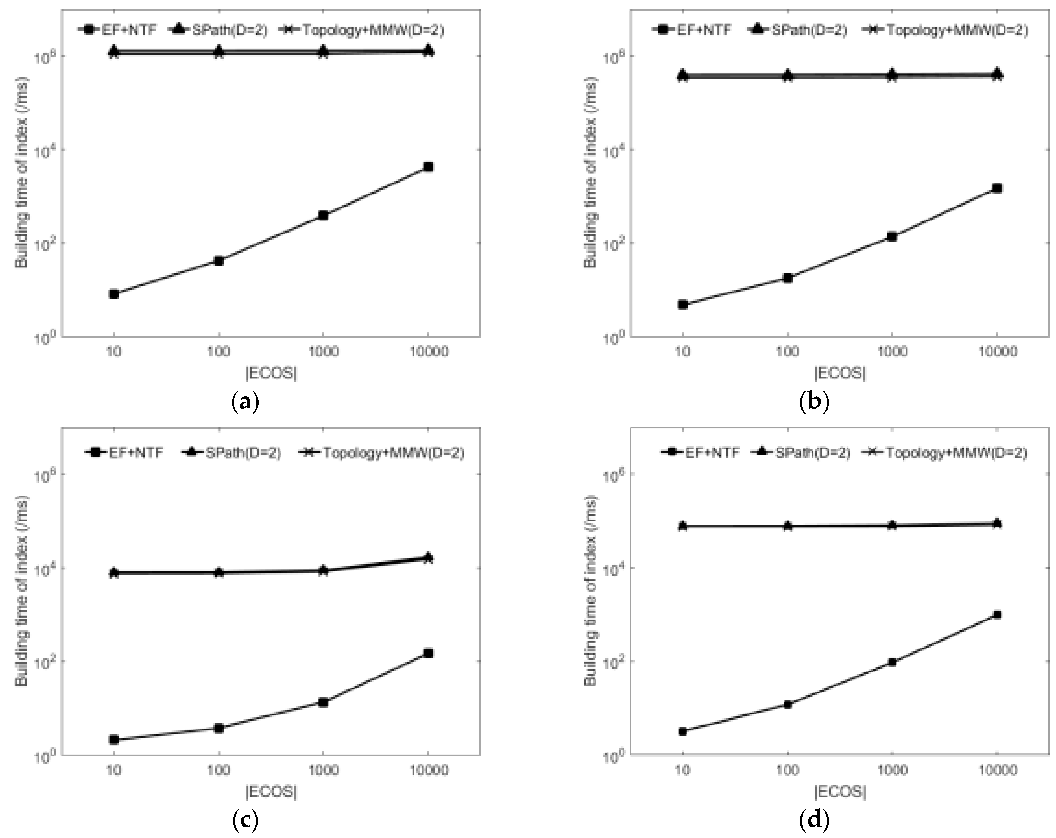
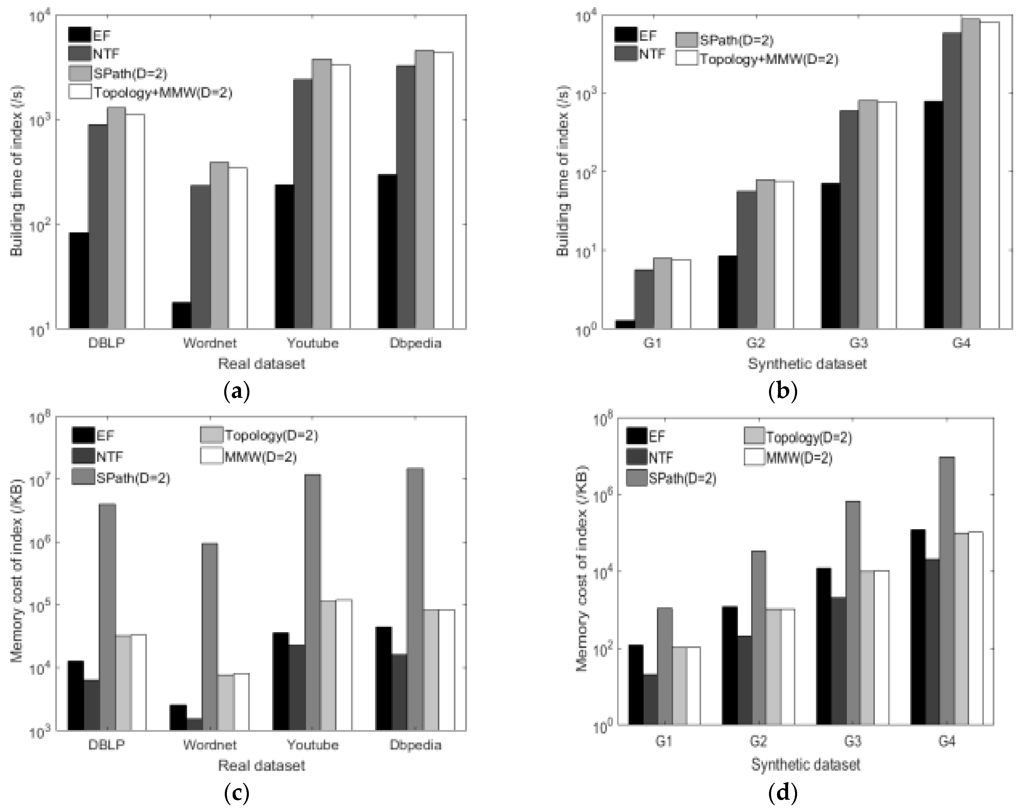
6.2.1. Construction Time and Memory Cost of Index

Figure 8a,b show the comparisons of construction time for different indexes on synthetic datasets and different real datasets. The RAM algorithm needs to construct the SPath index, and the RWM algorithm constructs the Topology and MMW index. We find that the construction time of each index increases as the graph scale increases. The construction time of the EF index is much smaller than others, because it only needs to sort edges of different labels, without having to compute complex node relationships. The NTF index is significantly better than the Topology + MMW (D = 2) and SPath index, because the NTF index only needs to traverse the data graph once to obtain the relationships among all nodes and their adjacency nodes. In addition, the Topology + MMW (D = 2) and SPath index are constrained by D, and the construction time of index will grow exponentially with increasing D.

Figure 8c,d show the comparisons of memory cost for different indexes on the synthetic datasets and different real datasets. The memory cost of each index increases as the graph scale increases. We observe that the NTF and EF indexes account for less memory, because the NTF index only needs to store the degree of each node and the information of the next jump adjacency node, and the EF index only records the weight of each edge. But SPath, MMW, and Topology, according to different D, need to record the information of multi-hop adjacent nodes, for the memory cost of indexes will grow exponentially with increasing D.

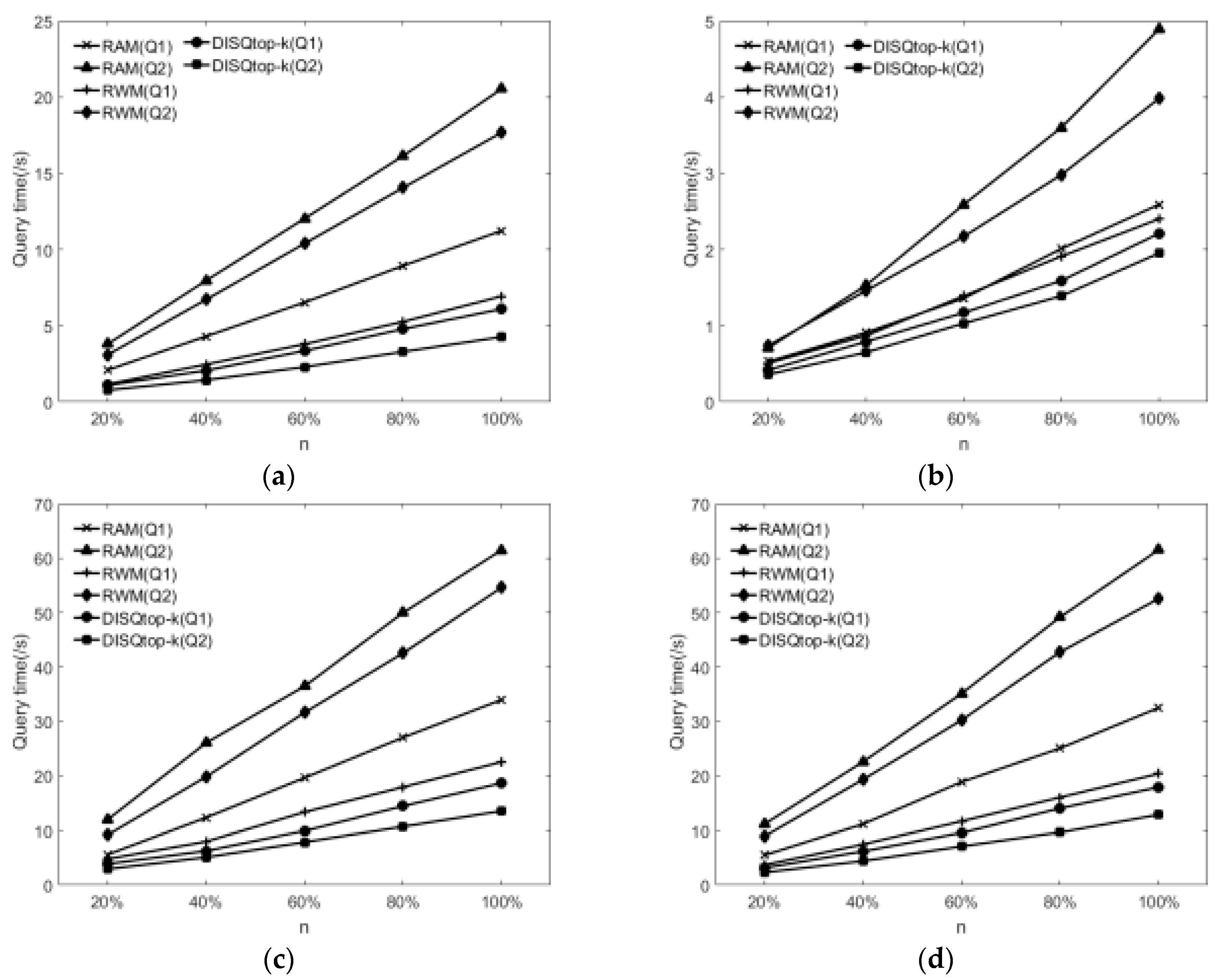
6.2.2. Interesting Subgraph Query Efficiency Evaluation

Figure 9a–d show the comparison of the query time based on the different real datasets when K = 10. We abstract each dataset into a data graph G. The parameter n (n = 20%, 40%, 60%, 80%, 100%) is the ratio of the nodes contained in the subgraph randomly extracted from the data graph G to the original data graph. In the experiment, for the unweighted query graph (Q₁) and weighted query graph (Q₂), we observe the query time of each algorithm is changed as the data graph scale increases. Among them, Q₁ is obtained when the query graph Q shown in Figure 2b removes weight, and Q₂ is the query graph Q shown in Figure 2b, and D = 2 in the index of RAM and RWM. For the weighted query graph, the algorithms of RAM and RWM need to query all the matching subgraphs and then to filter the subgraphs that do not meet weight limit conditions. But the DISQtop-k algorithm has filtered out the nodes and edges that do not meet conditions when the candidate set is filtered, which avoids the repeated calculation. So, the DISQtop-k algorithm runs faster and grows flatter. To ensure each query has at least one match result in the data graph, we generated every query graph by randomly extracting connected subgraph from the data graph.

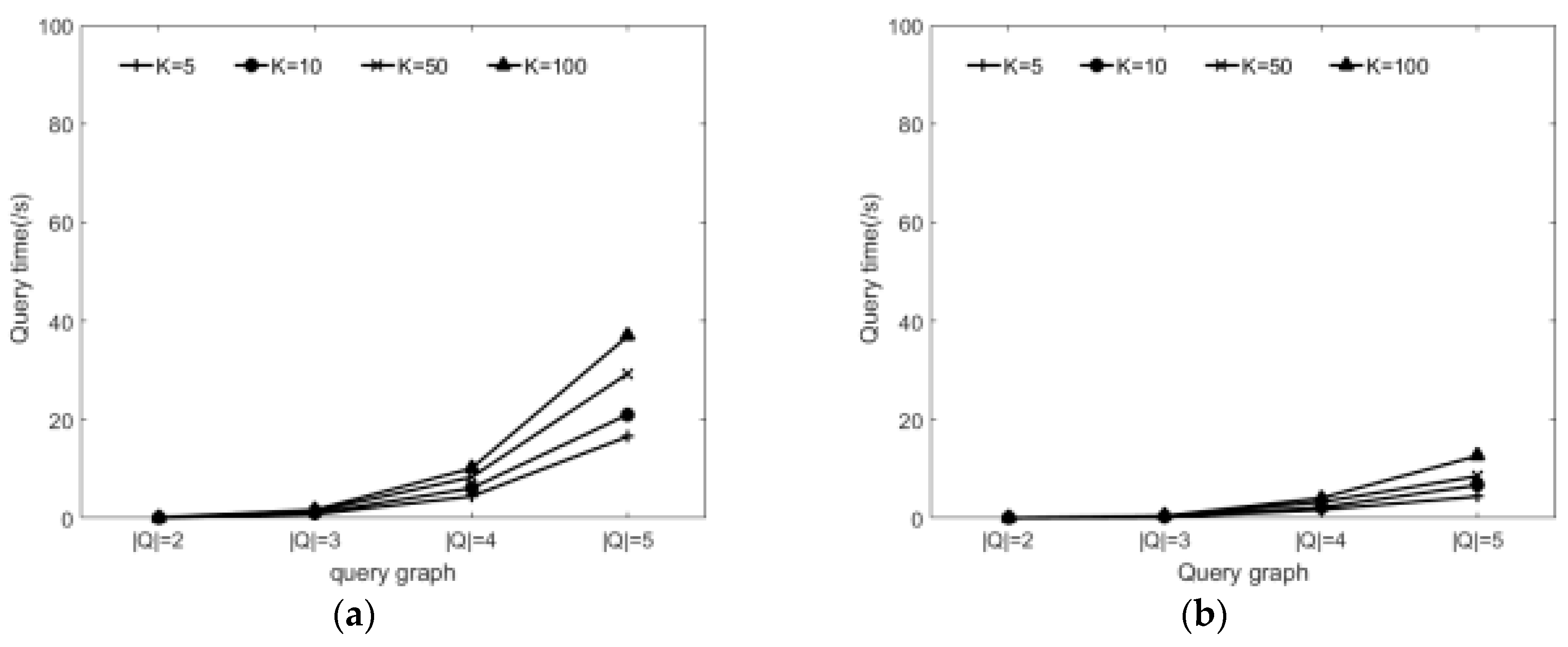
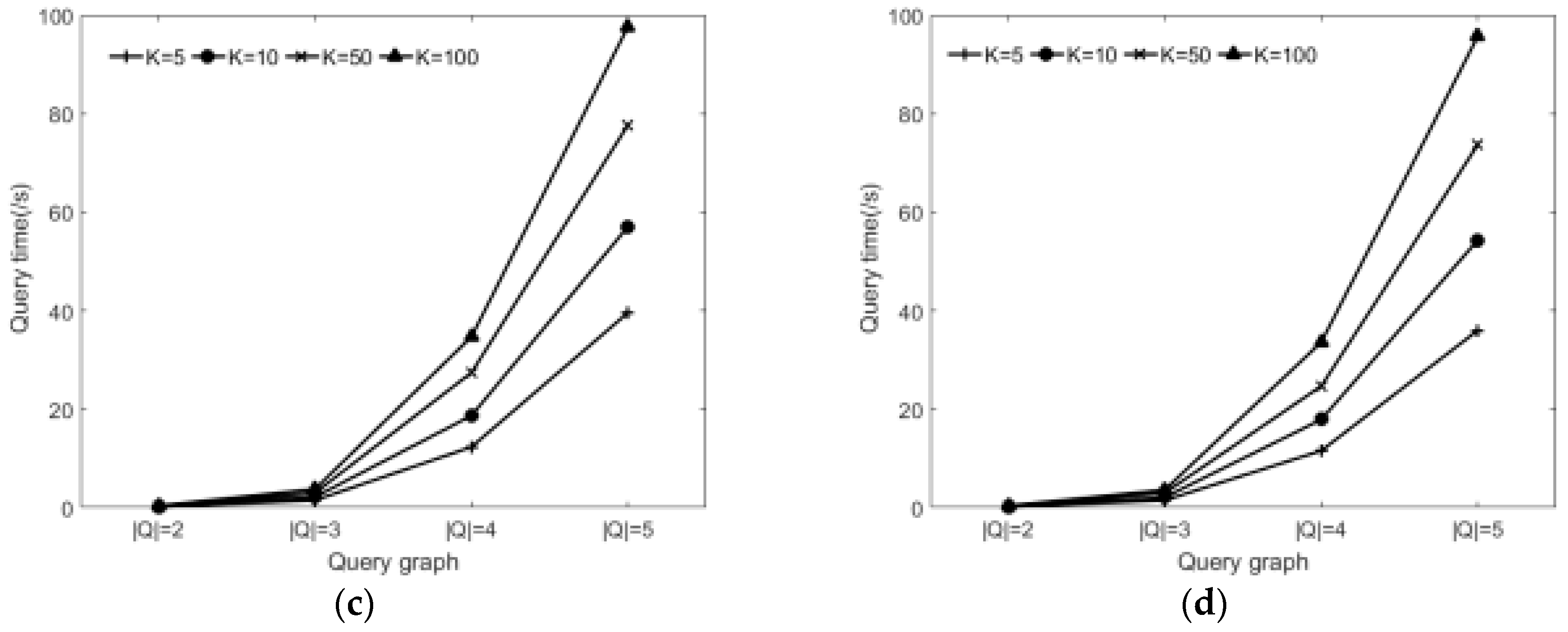
6.2.3. Effect of Varying Query Graph and the K

Figure 10a–d show effect of varying query graph and the K. From analysis we know that the node number of query graph and the setting of K value have some influence on the subgraph query time. Figure 10 shows the query time comparison of DISQtop-k for different scales of the query graph Q and varying K values. We find that the query time of each algorithm increases when increasing the query graph scale and K. The query time for varying K values is less volatile when the query graph Q is fixed. We also generated each query graph Q by randomly extracting connected subgraph from the data graph.

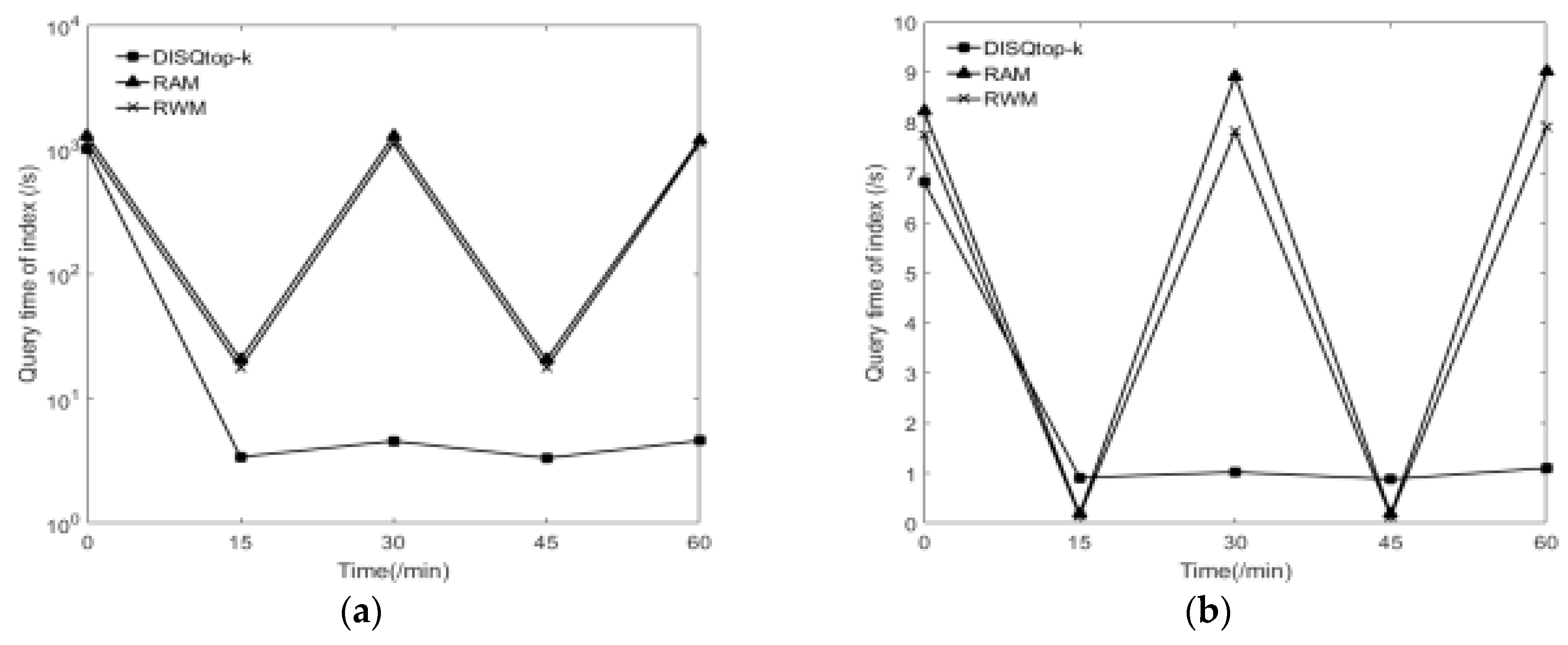
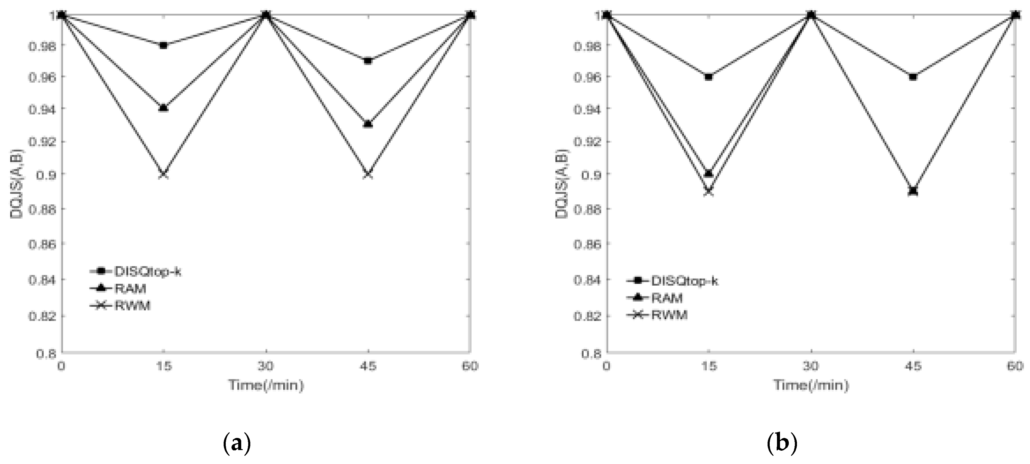
6.2.4. Effect of Dynamic Update and Query

Figure 11a–d show the comparison of index dynamic maintenance time when the ECOS of different scales is collected during the jump time ∆t of the sliding window. As shown in the figure, each index increases as the ECOS scale increases. For the update speed, EF + NTF index is obviously faster than Topology + MMW (D = 2) index and SPath index. Because the DISQtop-k algorithm directly stores the data graph in the EF index and NTF index, and it only needs to update the ECO directly in the ECOS to the EF index and the NTF index when indexes are dynamically updated. However, there is no dynamic processing mechanism in RWM and RAM algorithms, so dynamic query can only be realized by the static processing method and indexes need to be recreated every time indexes are updated dynamically.

Figure 12a,b show the dynamic query efficiency on the synthetic dataset G₁ and real dataset DBLP. Figure 13a,b show the accuracy of the dynamic query on the synthetic dataset G₁ and real dataset DBLP. Here, the query interval is 15 min, the sliding window is 30 min, the sliding window jumps every 10 min (∆t), the query graph Q is shown in Figure 2b, and D = 2 in the index of RAM and RWM. The start time of the sliding window and the first query are at 0. To measure the accuracy of the dynamic query, we define a metric: dynamic query jaccard similarity (DQJS) based on the classical Jaccard similarity.

$$\mathrm{DQJS}\left(\mathrm{A},\mathrm{B}\right)=\frac{A{\displaystyle \cap }\text{}B}{A{\displaystyle \cup }\text{}B}$$

(3)

A represents the result set of the dynamic approximate query, and B represents the result set of the static exact query. In every ∆t, we randomly add 100 ECOs. We find that the dynamic query time of DISQtop-k algorithm must be much smaller than that of RWM and RAM algorithms when the query time is the same as the jump time of the sliding window, namely, to query at the time ∆t. Although the DISQtop-k algorithm needs to obtain the intermediate result CE from the dynamically updated EF index and NTF index and then obtain the matching result, the efficiency of index update and subgraph query is obviously better than that of RWM and RAM algorithms. When the query time is the different from the jump time of the sliding window, namely, to query during the time ∆t, although the dynamic query time of DISQtop-k algorithm is not necessarily smaller than that of RWM and RAM, the accuracy of RWM and RAM algorithms are inferior to the DISQtop-k algorithm. Because to try to ensure the accuracy of the query, the DISQtop-k algorithm adopts the sliding window mechanism and obtains the matching subgraph by calculating the intermediate results, which considers partial updates after the last moment, but RWM and RAM only use the updated index on the last moment to query, which does not consider any updates after the last moment. So, the accuracy of RWM and RAM algorithms are inferior to the DISQtop-k algorithm. Specially, the accuracy is 1 when the time is 30 min, that is because we set the size of the sliding window is 30 min, all three algorithms are accurate query rather than approximate query at that time.

7. Conclusions

In this paper, we present a Top-K interesting subgraph query method, namely DISQtop-k method. In this method, first, GTSF index composed of NTF index and EF index is proposed, and multi-factor candidate set filtering strategy is proposed based on GTSF index, which can effectively prune the candidate set of the query graph. Then, the candidate set is initially matched and dynamically modified to obtain the continuous query results by using the sliding window technique and considering the query error resulting from dynamic changes of the graph. Finally, a graph change optimization mechanism (IDM) is proposed to reduce redundant updates, and the index is dynamically maintained based on IDM. The experimental results of real and synthetic datasets show that DISQtop-k has high query efficiency on large-scale dynamic labeled graphs, and the query results have certain practical significance.

References

1. Sonmez, A.B.; Can, T. Comparison of tissue/disease specific integrated networks using directed graphlet signatures. Bmc Bioinf. 2017, 18, 135. [Google Scholar] [CrossRef] [PubMed]
2. Li, X.J.; Yang, G.H. Graph Theory-Based Pinning Synchronization of Stochastic Complex Dynamical Networks. IEEE Trans. Neural Netw. Learn Syst. 2017, 28, 427–437. [Google Scholar] [CrossRef] [PubMed]
3. Ma, S.; Li, J.; Hu, C.; Lin, X.; Huai, J. Big Graph Search: Challenges and Techniques. Front. Comput. Sci. 2016, 10, 387–398. [Google Scholar] [CrossRef]
4. Wu, B.; Shen, H. Exploiting Efficient Densest Subgraph Discovering Methods for Big Data. IEEE Trans. Big Data. 2017, 3, 334–348. [Google Scholar] [CrossRef]
5. Zhang, H.W.; Xie, X.F.; Duan, Y.Y.; Wen, Y.L. An algorithm for subgraph matching based on adaptive structural summary of labeled directed graph data. Chin. J. Comput. 2017, 40, 52–71. [Google Scholar] [CrossRef]
6. Lee, J.; Han, W.S.; Kasperovics, R.; Lee, J.H. An in-depth comparison of subgraph isomorphism algorithms in graph databases. Proc. VLDB Endowment 2012, 6, 133–144. [Google Scholar] [CrossRef]
7. Kim, J.; Shin, H.; Han, W.S.; Hong, S. Taming Subgraph Isomorphism for RDF Query Processing. Proc. VLDB Endowment 2015, 8, 1238–1249. [Google Scholar] [CrossRef]
8. Shang, H.C.; Zhang, Y.; Lin, X.M.; Yu, J.X. Taming verification hardness: An efficient algorithm for testing subgraph isomorphism. Proc. VLDB Endowment 2008, 1, 364–375. [Google Scholar] [CrossRef]
9. Yan, X.; He, B.; Zhu, F.; Han, J. Top-K aggregation queries over large networks. In Proceedings of the IEEE International Conference on Data Engineering, California, CA, USA, 1–6 March 2010; pp. 377–380. [Google Scholar] [CrossRef]
10. Gupta, M.; Gao, J.; Yan, X.; Cam, H. Top-K interesting subgraph discovery in information networks. In Proceedings of the International Conference on Data Engineering, Chicago, IL, USA, 31 March–4 April 2014; pp. 820–831. [Google Scholar] [CrossRef]
11. Fan, W.; Wang, X.; Wu, Y. Diversified top-k graph pattern matching. Proc. VLDB Endowment 2013, 6, 1510–1521. [Google Scholar] [CrossRef]
12. Ju, W.; Li, J.; Yu, W.; Zhang, R. iGraph: An incremental data processing system for dynamic graph. Front. Comput. Sci. 2016, 10, 462–476. [Google Scholar] [CrossRef]
13. Zhang, L.; Lin, J.; Karim, R. Sliding Window-Based Fault Detection From High-Dimensional Data Streams. IEEE Trans. Syst. Man Cybern. Syst. 2017, 47, 289–303. [Google Scholar] [CrossRef]
14. Wang, X.; Zhang, Y.; Zhang, W.; Lin, X. Skype: Top-k spatial-keyword publish/subscribe over sliding window. Proc. VLDB Endowment 2016, 9, 1–26. [Google Scholar] [CrossRef]
15. Ullmann, J.R. An Algorithm for Subgraph Isomorphism. J. ACM 1976, 23, 31–42. [Google Scholar] [CrossRef]
16. Cordella, L.P.; Foggia, P.; Sansone, C.; Vento, M. A (sub)graph isomorphism algorithm for matching large graphs. IEEE Trans. Pattern Anal. Mach. Intell. 2004, 26, 1367–1372. [Google Scholar] [CrossRef] [PubMed]
17. Sun, Z.; Wang, H.; Wang, H.; Shao, B.; Li, J. Efficient subgraph matching on billion node graphs. Proc. VLDB Endowment 2012, 5, 788–799. [Google Scholar] [CrossRef]
18. Han, W.S.; Lee, J.; Lee, J.H. TurboISO: Towards ultrafast and robust subgraph isomorphism search in large graph databases. In Proceedings of the 2013 ACM SIGMOD International Conference on Management of Data, New York, NY, USA, 22–27 June 2013; pp. 337–348. [Google Scholar] [CrossRef]
19. Ren, X.; Wang, J. Exploiting Vertex Relationships in Speeding up Subgraph Isomorphism over Large Graphs. Proc. VLDB Endowment 2015, 8, 617–628. [Google Scholar] [CrossRef]
20. Bi, F.; Chang, L.; Lin, X.; Qin, L.; Zhang, W. Efficient Subgraph Matching by Postponing Cartesian Products. In Proceedings of the 2016 International Conference on Management of Data, San Francisco, CA, USA, 26 June–1 July 2016; pp. 1199–1214. [Google Scholar] [CrossRef]
21. Holder, L.B.; Cook, D.J.; Djoko, S. Substructure discovery in the SUBDUE system. In Proceedings of the 3rd International Conference on Knowledge Discovery and Data Mining, Seattle, WA, USA, 31 July–1 August 1994; pp. 169–180. [Google Scholar]
22. Zhu, F.D.; Qu, Q.; Lo, D.; Yan, X.; Han, J.; Yu, P.S. Mining Top-K large structural patterns in a massive network. Proc. VLDB Endowment 2011, 4, 807–818. [Google Scholar]
23. Zhao, P.X.; Han, J.W. On graph query optimization in large networks. Proc. VLDB Endowment 2010, 3, 340–351. [Google Scholar] [CrossRef]
24. He, H.; Singh, A.K. Query language and access methods for graph databases. In Proceedings of the Acm Sigmod International Conference on Management of Data, Indianapolis, IN, USA, 6–11 June 2010; pp. 125–160. [Google Scholar] [CrossRef]
25. Pietracaprina, A.; Riondato, M.; Upfla, E.; Vandin, F. Mining top-k frequent itemsets through progressive sampling. Data Min. Knowl. Discovery 2010, 21, 310–326. [Google Scholar] [CrossRef]
26. Wu, C.W.; Shie, B.E.; Tseng, V.S.; Yu, P.S. Mining top-k high utility itemsets. In Proceedings of the 18th ACM International Conference on Knowledge Discovery and Data Mining, Beijing, China, 12–16 August 2012; pp. 78–86. [Google Scholar] [CrossRef]
27. Yang, Z.; Fu, W.C.; Liu, R. Diversified Top-k Subgraph Querying in a Large Graph. In Proceedings of the 2016 International Conference on Management of Data, San Francisco, CA, USA, 26 June–1 July 2016; pp. 1167–1182. [Google Scholar] [CrossRef]
28. Wang, L.; Han, J.; Chen, H.; Lu, J. Top-k probabilistic prevalent co-location mining in spatially uncertain data sets. Front. Comput. Sci. 2016, 10, 488–503. [Google Scholar] [CrossRef]
29. Zhang, X.; Meng, X. Discovering top-k patterns with differential privacy-an accurate approach. Front. Comput. Sci. 2014, 8, 816–827. [Google Scholar] [CrossRef]
30. Sha, C.; Wang, K.; Zhang, D.; Wang, X.; Zhou, A. Optimizing top-k retrieval: submodularity analysis and search strategies. Front. Comput. Sci. 2016, 10, 477–487. [Google Scholar] [CrossRef]
31. Xu, J.; Zhang, Q.Z.; Zhao, X.; Lu, P.; Li, T.S. Survey on Dynamic Graph Pattern Matching Technologies. J. Softw. 2018, 29, 663–688. [Google Scholar] [CrossRef]
32. Wang, S.P.; Wen, Y.Y.; Zhao, H.; Meng, Y.H. An Incremental Processing Algorithm about Disjoint Query Based on Sliding Window over Data Stream. Chin. J. Comput. 2017, 40, 2381–2403. [Google Scholar] [CrossRef]
33. Wang, W.P.; Li, J.Z.; Zhang, D.D.; Guo, L.J. Sliding Window Based Method for Processing Continuous J-A Queries on Data Streams. J. Softw. 2006, 17, 740–749. [Google Scholar] [CrossRef]
34. Khan, A.; Wu, Y.; Aggarwal, C.C.; Yan, X. NeMa: Fast graph search with label similarity. In Proceedings of the International Conference on Very Large Data Bases, Riva del Garda, Italy, 26–30 August 2013; pp. 181–192. [Google Scholar] [CrossRef]
35. Sun, Y.Z.; Yu, Y.T.; Han, J.W. Ranking-Based clustering of heterogeneous information networks with star network schema. In Proceedings of the ACM SIGKDD International Conference on Knowledge Discovery and Data Mining, Paris, France, 29 June–2 July 2009; pp. 797–806. [Google Scholar] [CrossRef]
36. Chakrabarti, D.; Zhan, Y.; Faloutsos, C. R-MAT: A recursive model for graph mining. In Proceedings of the Fourth SIAM International Conference on Data Mining, Lake Buena Vista, FL, USA, 22–24 April 2004; pp. 442–446. [Google Scholar]
Figure 1. Example of undirected weighted labeled graph G.
Information 10 00061 g001
Figure 2. Matching subgraph P1 and P2 of Q. (a) data graph G; (b) query graph Q.
Information 10 00061 g002
Figure 3. Node topology feature (NTF) index for G in Figure 1.
Information 10 00061 g003
Figure 4. Edge feature (EF) index for G in Figure 1.
Information 10 00061 g004
Figure 5. The candidate node set of Q in Figure 2.
Information 10 00061 g005
Figure 6. The candidate edge set of Q in Figure 2.
Information 10 00061 g006
Figure 7. The change process of initial Top-K heap and the candidate matching heap CM.
Information 10 00061 g007
Figure 8. Comparison of construction time and memory cost for indexes. (a) Comparison of construction time in real datasets; (b) Comparison of construction time in synthetic datasets; (c) Comparison of memory cost in real datasets; (d) Comparison of memory cost in synthetic datasets.
Information 10 00061 g008
Figure 9. Comparison of query time for different algorithms. (a) Comparison of query time in DataBase systems and Logic Programming (DBLP); (b) Comparison of query time in Wordnet; (c) Comparison of query time in Youtube (d) Comparison of query time in Dbpedia.
Information 10 00061 g009
Figure 10. Effect of varying query graph and the K. (a) Comparisons in DBLP; (b) Comparisons in Wordnet; (c) Comparisons in Youtube (d) Comparisons in Dbpedia.
Information 10 00061 g010aInformation 10 00061 g010b
Figure 11. The comparison of index dynamic maintenance time. (a) Comparisons in DBLP; (b) Comparisons in Wordnet; (c) Comparisons in synthetic dataset G1 (d) Comparisons in synthetic dataset G2.
Information 10 00061 g011
Figure 12. The comparison of the dynamic query efficiency. (a) Comparisons in the real dataset DBLP; (b) Comparisons in the synthetic dataset G1.
Information 10 00061 g012
Figure 13. The comparison of the accuracy for dynamic query. (a) Comparisons in the real dataset DBLP; (b) Comparisons in the synthetic dataset G1.
Information 10 00061 g013