Article

A Method for Road Extraction from High-Resolution Remote Sensing Images Based on Multi-Kernel Learning

1
College of Information Science and Engineering, Fujian University of Technology, Fuzhou 350118, China
2
College of Tourism, Fujian Normal University, Fuzhou 350117, China
*
Author to whom correspondence should be addressed.
Information 2019, 10(12), 385; https://doi.org/10.3390/info10120385
Submission received: 31 October 2019 / Revised: 21 November 2019 / Accepted: 2 December 2019 / Published: 6 December 2019

Abstract

:
Extracting road from high resolution remote sensing (HRRS) images is an economic and effective way to acquire road information, which has become an important research topic and has a wide range of applications. In this paper, we present a novel method for road extraction from HRRS images. Multi-kernel learning is first utilized to integrate the spectral, texture, and linear features of images to classify the images into road and non-road groups. A precise extraction method for road elements is then designed by building road shaped indexes to automatically filter out the interference of non-road noises. A series of morphological operations are also carried out to smooth and repair the structure and shape of the road element. Finally, based on the prior knowledge and topological features of the road, a set of penalty factors and a penalty function are constructed to connect road elements to form a complete road network. Experiments are carried out with different sensors, different resolutions, and different scenes to verify the theoretical analysis. Quantitative results prove that the proposed method can optimize the weights of different features, eliminate non-road noises, effectively group road elements, and greatly improve the accuracy of road recognition.

1. Introduction

Road is an important geographic information resource. The correct and effective extraction of road plays an important role in geographic information system (GIS) database updates, image registration, navigation, information fusion, change detection, etc. [1,2,3]. Extracting road from high resolution remote sensing (HRRS) images is an economic and effective way to acquire road information. Road extraction has become a research hotspot in the field of remote sensing imagery processing, but it is still an unsolved research topic. On the one hand, the objects on the ground have diverse and complex spectral features, some of which may have similar spectral appearances to the road, making it difficult to distinguish the road from non-road [4]. On the other hand, noises like the shadows of trees, buildings on roadsides, and the vehicles on the road can be observed from high-resolution imagery. Thus, extracting smooth and complete road areas from HRRS images remains a challenging and tricky topic [5].
Great attention has been plaid to research on road extraction from HRRS images and various methods have been proposed over the past decades. Some comprehensive reviews can be found in [6,7]. The methods have been founded in diverse image processing technologies, including classification [6,8,9], segmentation [10,11,12], linear feature based extraction [13,14,15], template matching [16,17,18], etc. Most of the popular methods rely on classification, which can be divided into supervised classification and unsupervised classification. While the unsupervised classification method enjoys a higher degree of automation, supervised classification method is more adaptable and efficient and has become the mainstream method for extracting information from remote sensing images. The support vector machine (SVM), a powerful tool in classification, has been widely used in road extraction [19]. In general, SVM has better performance than similar algorithms [20], and representative methods adopting SVM are as follows.
(1)
Pixel-spectral classification (PSC) [21] is widely used in early road extraction; this method classifies an image into the road group and the non-road group according to the pixel spectral information of the image.
(2)
Spectral-spatial classification (SSC) [9] is a two-step method for extracting road skeleton from HRRS images. In the first step, a feature vector is constructed by integrating spectral–spatial classification and shape features. The SVM classifier is used to segment the imagery into two classes: The road class and the non-road class. In the second step, the road class is refined by utilizing homogenous and shape features.
(3)
Region-based classification (RBC) [22] is a semi-automatic approach that first segments the image and combines adjacent segments by Full Lambda Schedule. The SVM classifier is then used to classify the segmented region by spatial, spectral, and textural features of the image, and the initial road skeleton is obtained. Finally, the quality of the detected road skeleton is improved by using morphological operators.
It is worth mentioning that in recent years, convolution neural networks (CNN) have made great progress in image classification tasks [23,24,25]. The CNN can reduce false detections by embedding much high-level and multi-scale information [26,27]. Especially when extracting roads from HRRS images with complex backgrounds, CNN has obvious advantages, but its classifier needs to be trained through a large number of labeled samples, and manually labeling samples is time-consuming and laborious. A large number of training samples with different resolutions and different scenes are often difficult to obtain [28]. The goal of the research on road extraction from HRRS images is to obtain a large amount of classified data through a small number of labelled samples.
The existing road extraction methods are mostly directed to a specific type of image that is highly dependent on data. Besides this, the road information on the HRRS images is not fully utilized. As a result, most of the existing road extraction models are not adaptable or applicable. Overall, no breakthrough progress has been made. To fill the knowledge gap, this study first adopts multi-kernel learning to effectively integrate the spectral features, texture features, and linear features of images to enhance the adaptability of the algorithm. Road skeleton is then refined by a set of suitable post processing stages. A global road connection model based on the prior knowledge and topological features of the road is designed to further connect road elements to form a complete road network. By designing a novel method of road extraction from HRRS images, this paper aims to improve the adaptability and applicability of the road extraction method.
Accordingly, this paper is organized as follows. Section 2 presents the new method to extract road from HRRS images, while experimental results are reported in Section 3, and a conclusion is presented in Section 4.

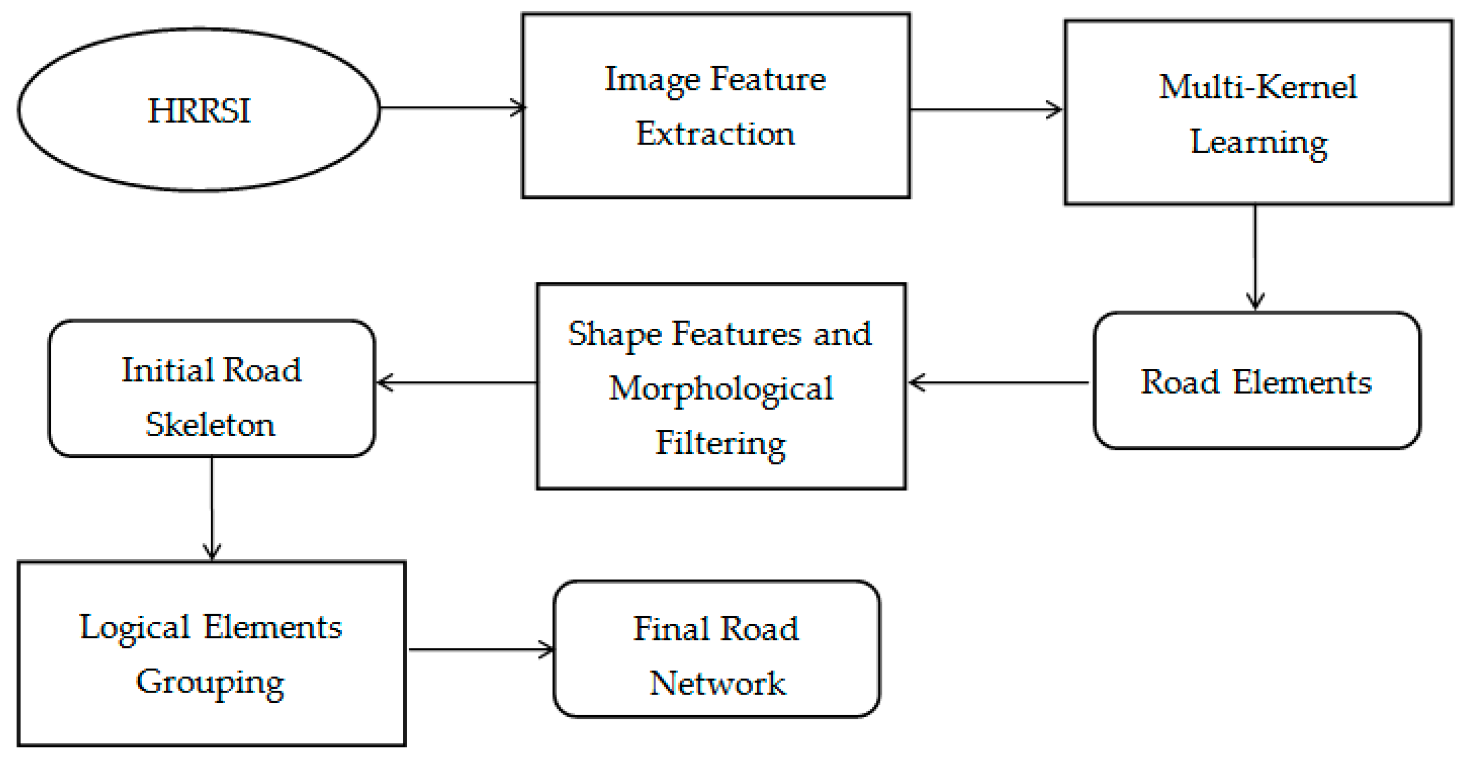
2. Proposed Methodology

The objective of this study is to design an efficient approach to extract an accurate road network from HRRS images. Figure 1 summarizes the main processing steps of the proposed method. As shown in this figure, the method mainly consists of the following four steps.
(1)
The features of the road in HRRS images and extract image features suitable for describing road are analyzed. Multi-scale and multi-direction non-subsampled contourlet transform (NSCT) is used to describe the texture features and linear features of the road. A color moment matrix is used to describe the spectral feature.
(2)
Road elements are roughly extracted by multi-kernel learning and multi-feature fusing (MKL). About 8% of the road samples and 10% of the non-road samples are taken for classification learning, and the MKL-SVM classifier is obtained to divide the image into two categories: Road and non-road. This step provides candidate road elements.
(3)
Road elements are precisely extracted by road shape features and morphological filtering. This step combines such features as the slenderness of the road’s shape, the compactness of ground objects, and the area of surroundings to build road shape indexes for automatically filtering out the interference of non-road noises. A series of morphological operations are also carried out to regulate the incomplete structures of the road elements. This step provides the initial road skeleton.
(4)
Road elements are grouped by the road element connection penalty factor, which is constructed based on the prior knowledge and topological features of the road. This step obtains the connected and complete road network.
Details of each step are described in the following sections.

2.1. Image Features Extraction

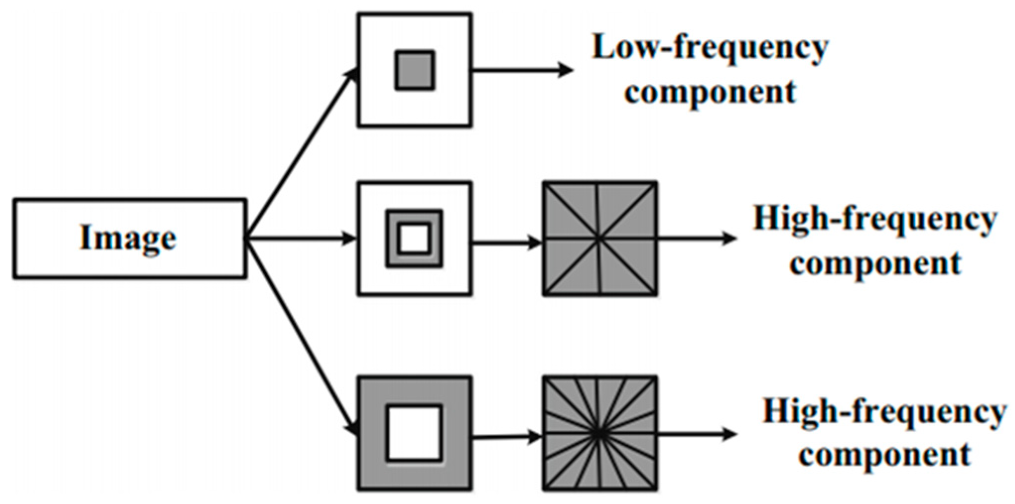
2.1.1. Non-Subsampled Contourlet Transform

Non-subsampled contourlet transform (NSCT) is a fully shift-invariant, multi-scale, and multi-direction transform and is an expansion of the contourlet transform proposed by Cunha et al. [29]. NSCT offers a high degree of directionality and anisotropy, and it is capable of modeling the dependencies across directions, scales, and space. Thus, NSCT is a true two-dimensional representation of images. NSCT uses the non-subsampled pyramids (NSP) and the non-subsampled directional filter banks (NSDFB) to obtain multi-scale and multi-directional decompositions of the image without down-sampling or up-sampling. An example of the decomposition process of NSCT is given in Figure 2.
The road has important geometric characteristics such as multi-scale, multi-directional, and unique curve features. There are several advantages of NSCT expressing the road features. (1) NSCT has a delicate ability to identify directions. (2) For the multi-scale features of roads, NSCT is capable of continuously characterizing images from different scales. (3) NSCT can express the curve in the image very well. (4) NSCT is the inheritance and development of the standard contourlet transform, which can be regarded as a contourlet transform with translation-invariant properties.
In view of the above analysis, this paper adopts NSCT transform to make NSCT decomposition on HRRS images based on the deep analysis of road features, and obtains information of multi-directional sub-bands at different scales. Then, a statistical model is constructed by analyzing each sub-band coefficient. The low frequency sub-band and high frequency sub-band feature vectors are constructed, respectively, so as to reasonably express the deep image features of the road.
  • Features of low frequency sub-band.
    (1)
    Mean
    μ L o w = 1 M N x = 1 M y = 1 N I L o w ( x , y )
    In Equation (1), ILow(x,y) denotes the matrix of low frequency sub-band coefficients, M, N denotes the number of rows and columns of coefficients in the sub-band respectively, M, and N is the dimension of the coefficient matrix.
    (2)
    Variance
    δ L o w = 1 M N x = 1 M y = 1 N [ I L o w ( x , y ) μ L o w ] 2
    (3)
    Homogeneity
    h L o w = x = 1 M y = 1 N I L o w ( x , y ) 1 + ( x y ) 2
    The low frequency sub-band reflects the information of the image’s basic features. The texture feature vector constructed by the mean (μLow), the variance (δLow), and the homogeneity (hLow) can be expressed as:
    F 1 = [ μ L o w , δ L o w , h L o w ]
  • Features of high frequency sub-band.
    After the image is transformed by NSCT, multi-directional high frequency sub-bands of different scales are obtained. The coefficient magnitude sequence of these sub-bands is calculated as the features of high frequency sub-bands.
    (1)
    Gradient energy
    E H = 1 M N x = 1 M y = 1 N { [ I H ( x , y ) I H ( x 1 , y ) ] 2 + [ I H ( x , y ) I H ( x , y 1 ) ] 2 }
    (2)
    Variance
    δ H = 1 M N x = 1 M y = 1 N [ I H ( x , y ) μ H ] 2 ,
    where μH is the mean value of the high frequency sub-bands.
Let the number of direction filters used by layer i be ni (i∈[1, L]), and the layer i generates 2 n i multi-directional sub-bands. The sub-image obtained through NSCT decomposition of L Layers is
{ B A N D 1 ( 1 ) , , B A N D i ( 1 ) , B A N D i ( 2 ) , B A N D i ( 2 n i ) , , B A N D L ( 2 n L ) } i = 1 L
In order to effectively express the special features of spectral–texture fusion and to reduce the texture feature dimension so as to improve the speed of recognition, the 2 n i directional sub-band features of each layer are counted as the feature of this layer. F(i) represents the statistical characteristics of all directions of the layer i. F(i) is defined as:
F ( i ) = 1 2 n i k = 1 2 n i ( B A N D i ( k ) )
which can be used to calculate the textural features of the high frequency sub-bands of each layer. The dimension of features is reduced while considering the directional features of each layer. The high frequency sub-band reflects the detailed information of the image. The texture feature vector constructed by the high frequency sub-band gradient energy and the high frequency sub-band coefficient variance can be expressed as:
F 2 = [ E H 1 , δ H 1 , E H 2 , δ H 2 , , E H L , δ H L ]

2.1.2. Spectral Feature Extraction

Spectral feature is an important visual attribute of remote sensing images, and each object on the ground has its own unique spectral feature. A spectral feature has high stability and strong robustness of image scaling and rotation. In this paper, the color space of the image is first converted from RGB(Red, Green, Blue) to HSV(Hue, Saturation, Value), and then the three components of H, S, and V are converted into one-dimensional feature vectors. The corresponding histogram [30] is
p ( k ) = n k N    k = 0 , 1 , , L
where k is the value of the color feature and L is the maximum value of k. nk indicates the number of pixels whose color feature value is k in the image, and N is the total number of pixels of the image. By Equation (10), each feature parameter [31] is defined as follows:
μ 1 = i = 0 G i p ( i ) σ 2 = i = 0 G ( i μ 1 ) 2 p ( i ) μ 2 = σ 3 i = 0 G ( i μ 1 ) 3 p ( i ) μ 3 = σ 4 i = 0 G ( i μ 1 ) 4 p ( i ) 3 e = i = 0 G [ p ( i ) ] 2 .
The color features can be expressed as:
F 3 = [ μ 1 , σ 2 , μ 2 , μ 3 , e ] .

2.2. Image Classification Based on Multi-Kernel Learning

Machine learning aims to extract the hidden patterns from data based on algorithms. Due to the rapid advance of technology and communication, these algorithms have drawn widespread attention and have been successfully applied to many real-world problems [32]. The machine learning approach can be applied to different optimization problems ranging from wind energy decision system [33], socially aware cognitive radio handovers [34], and truck scheduling at cross-docking terminals [35,36] to the sustainable supply chain network integrated with vehicle routing [37]. These studies proved that machine learning can adapt the environmental changes, creating its own knowledge base and adjusting its functionality to make dynamic data and network handover decisions. Therefore, this paper introduces the method of machine learning into the study of road extraction to improve the adaptability and applicability of the road extraction method and thus improve the accuracy of road information recognition.
The kernel method is a commonly used method in machine learning. SVM has proven to be an effective kernel method. Compared to single-kernel SVM, multi-kernel learning [38] can optimize the weights of different features. This paper optimizes the weights of different features in the training stage by the multi-kernel learning framework, and achieves the effective fusion of spectrum, texture, and direction information.
According to the property of the kernel function, the linear weighted combination of M kernel functions is still a kernel function [39], which can be expressed as:
K ( x i , x j ) = m = 1 M d m K m ( x i , x j ) , s . t .   d m 0   a n d   m = 1 M d m = 1 .
Equation (13) is a kernel function expression for multi-core learning, where Km denotes the kernel function of each feature, M denotes the number of base kernel functions, and dm denotes the coefficient of the linear combination. The MKL-SVM classifier [40] is thus designed as:
g ( x j ) = s i g n ( i = 1 N u m a i y i m = 1 M d m k m ( x i , x j ) + b )
where Km(xi,xj) represents the mth kernel function, g(xj) denotes the predicted label value for the image j, ai is the optimization parameter, yi denotes the label of the training sample, b denotes the optimal offset of the multi-core classification panel, and Num indicates the number of training samples. The windows scan the whole image with the pixel at the center. A trained MKL-SVM classifier is used to judge the central pixel, which is divided into two types: Road and non-road. The corresponding pixel assignment is as follows:
P ( x ) = { 1 i f   x   i s   c l a s s i f i e d   a s   r o a d , 0 o t h e r w i s e .

2.3. Road Skeleton Extraction Based on Shape Feature and Morphology

While the multi-kernel learning method can effectively eliminate most non-road areas and roughly extract road elements, misidentified roads still exist as remotely sensed imagery exhibits a complex spectral character. A refinement process is necessary to improve the accuracy of the road skeleton. First, the morphological skeleton is extracted by using a series of morphology operations, such as corrosion and open operation, which can effectively tackle issues such as holes in some road elements, loose connections between different pixels, and incomplete structures. Second, road shape features [41] can be used to filter false segments. These features can be measured by area, compactness, and length–width ratio, which are introduced as follows:
(1)
Roads do not have small areas and regions with small areas can be regarded as noise and should be removed.
(2)
Compactness is defined as 4 .π. A/P2, where P is the perimeter of the region and A is the area of the region. Compactness is in the range of (0, 1].
(3)
Roads are narrow and long. Length–width ratio is the aspect ratio of the minimum-enclosing rectangle.

2.4. Road Elements Grouping

The road network is a topologically connected space system. However, disturbances in the appearance of roads can interfere with the extraction and cause gaps between extracted road sections. In order to eliminate the error candidate road elements and bridge the gaps, a set of penalty factors is established for road element connection. The factors are as follows:
(1)
Distance, including absolute distance and vertical distance. The absolute distance is the distance between the two nearest end points of the two road elements. The vertical distance is the distance from the two nearest endpoints in the vertical direction between the two road elements. Both the absolute and the vertical distance should be lower than a threshold.
(2)
Width difference. The difference of average width between two adjacent elements should be lower than a threshold.
(3)
Direction difference. The direction of a road section is defined as the vector connecting the two end points of its center-line. The direction difference, that is, the angle between the direction vectors of the two road sections, should be lower than a threshold for the two road sections to be connected.
(4)
Homogeneity. The road has strong homogeneity. Considering the similar spectral characteristics of adjacent road elements, this paper defines homogeneity as the color mean of each element. Homogeneity difference of the adjacent elements should be lower than a threshold.
When there are more than two candidate elements, the connected elements can be selected by the penalty function (Equation (16)),
P i = L o c 0 L o c i D + θ i Θ + W i W + exp ( ( L e n g t h ( i ) ) L ) + μ * H o m i
where Pi represents the penalty function of the connected candidate element i, and D, Θ, W, L, and μ are the weight constants of each factor. Loc0 represents the endpoint coordinate of the element that has been identified as the road, and Loci is the nearest endpoint coordinate of candidate element i from Loc0, while ||Loc0Loci|| represents the Euclidean distance between the two endpoints. θi is the direction difference between the candidate element i and the identified road element. Wi is the width factor, reflecting the average width difference between the candidate element i and the identified road element. Length (i) represents the length of the candidate element i. Homi represents the homogeneity factor, which can be expressed as Min(Mean(Li), Mean(L0))/Max(Mean(Li), Mean(L0)), where Mean(Li), and Mean(L0) and represents the color mean of element i and element 0, respectively.

3. Experimental Results and Discussions

To validate the effectiveness and superiority of this method, the proposed approach has been applied to a set of scenes in four experiments. The four selected test images are of different sensors, different resolutions, and different scenes (including city block, suburban area, complex intersection, and university campus). These images include typical objects on the ground. Three representative road extraction methods designed by previous researchers are selected for comparative analysis from the perspective of three accuracy measures, completeness, correctness, and quality.

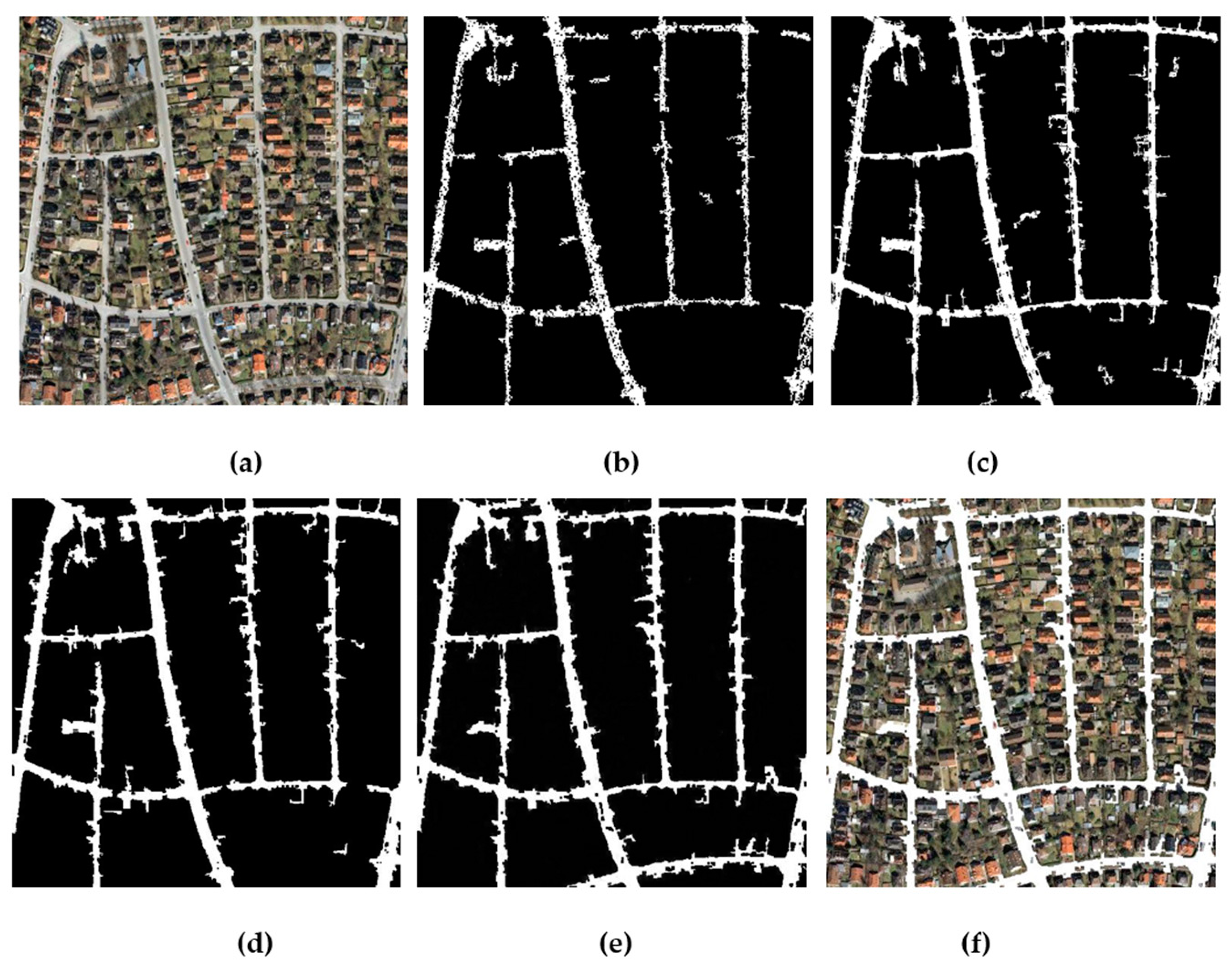
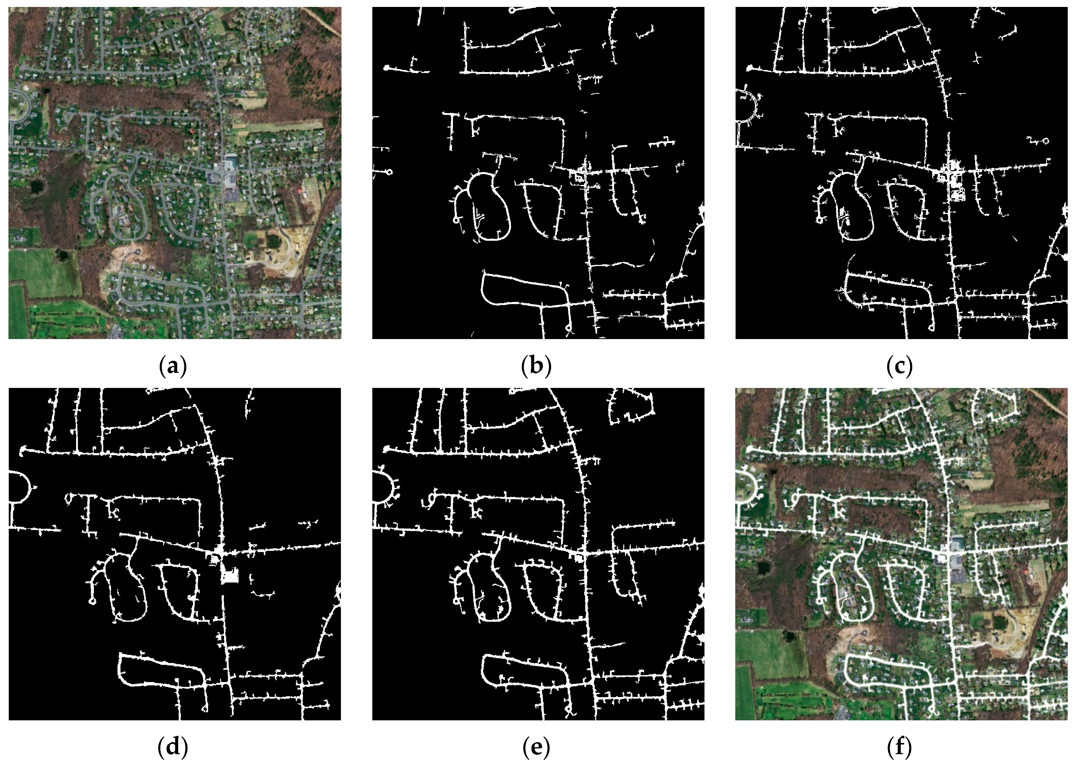
3.1. Tests of Different Study Areas
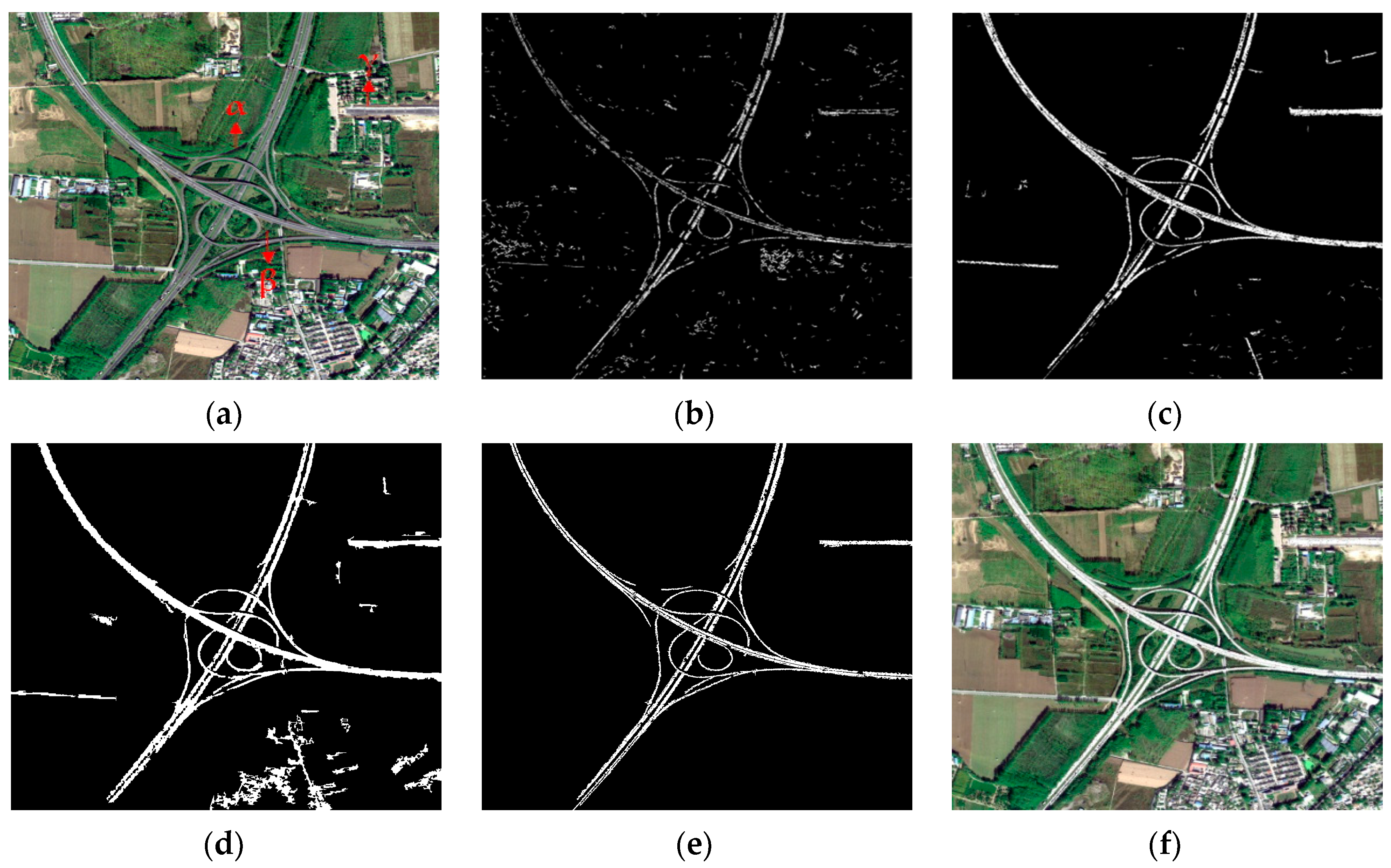
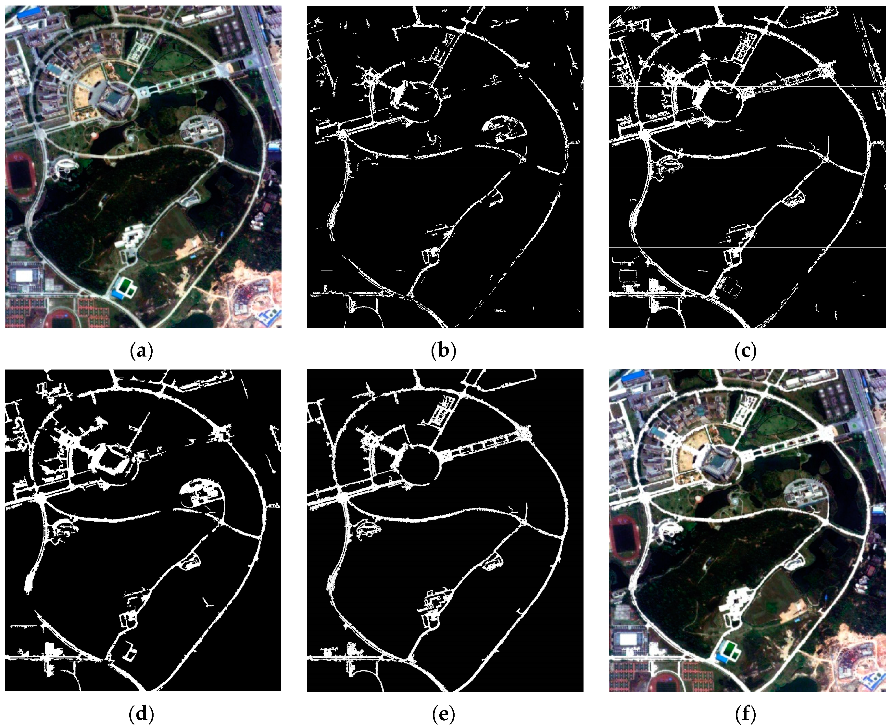
3.1.1. Study Area I

The first test image is downloaded from VPLab [42]. The study area has a spatial dimension of 512 × 512 pixels with three bands. The spatial resolution is 1 m per pixel. Figure 3a shows the study area of Experiment 1. Visual observation reveals that the selected test image (#1) belongs to a city block with a well-developed road network. Besides roads, other ground objects such as vegetation, shadows, vehicles, buildings, etc., can also be found in the study area. While part of the road surface is blocked by vegetation, shadows, or vehicles, the road network can still be clearly distinguished. Figure 3b–e show the results of extracting the road skeleton from #1 image by the PSC method, SSC method, RBC method, and the proposed method in this paper, respectively. It can be seen from a comparative analysis that the proposed method performs the best in maintaining the integrity of the road skeleton. The proposed method can effectively identify elements that cannot be identified by the PSC method, SSC method, or RBC method. Thus, the proposed method has a comparative advantage among the four methods.

3.1.2. Study Area II

In the second experiment, an image with a spatial size of 1500 × 1500 pixels, downloaded from [43], was used to test the performance of the proposed method, as shown in Figure 4a. Visual observation reveals that the selected test image (#2) belongs to the suburban area, which has various types of objects, including roads, buildings, parking lots, bare land, vegetation, waters, etc. Figure 4b–e show the results of extracting road skeleton from #2 image by the PSC method, SSC method, RBC method, and the proposed method in this paper, respectively. It is clear from the results that the PSC method can only extract an incomplete skeleton. While the SSC method is superior to the PSC method and RBC method in extracting complete skeletons, it has the shortfall of serious mis-extraction of phenomenon. As can be seen from the results, the proposed method can extract more complete and accurate road skeletons than the above three methods.

3.1.3. Study Area III

The third test image is a part of the suburb area of Beijing in 2011, which was recorded by the Worldview-II optical sensor. The study area has a spatial dimension of 3680 × 3140 pixels. The spatial resolution is 0.5 m per pixel, including three bands of red, green, and blue. Figure 5a shows the third test image (#3). The test image shows an area of a complex intersection. The main road is a two-way lane, and the isolation zone is clearly visible. There are eight auxiliary roads, two of which are seriously obstructed by vegetation. The two covered auxiliary roads are marked as “α” and “β”, respectively, in Figure 5a. Another main road that shares the same road width and pavement material with the intersection road is also the target of extraction in this experiment, marked as “γ” in Figure 5a. Figure 5b–e show the results of extracting road skeleton from #3 image by the PSC method, SSC method, RBC method, and the proposed method in this paper, respectively. It is clear from the results that the proposed method performs the best in extracting high-quality road skeleton, while the PSC method is the worst. The road skeleton extracted by the RBC method is complete, but due to the initial segmentation, the RBC method extracts two-way roads with serious adhesions, and the mis-extraction region is the most common among the four methods.

3.1.4. Study Area IV

The fourth test image is the WorldView-II image of the 1800 × 2100 pixels of Fuzhou University (Qishan Campus) in 2014, as shown in Figure 6a, marked as “#4”. The spatial resolution is 0.5 m per pixel, including three bands of red, green, and blue. The test image the main types of objects on the university campus, such as campus main roads, branch roads, teaching buildings, administrative buildings, libraries, campus squares, sports fields, stadiums, vegetation, waters, and unfinished construction projects. The #4 image experiment aims to extract campus road information from the new district of Fuzhou University. The road samples are only selected from the internal road surface of the campus. The results of the four methods of extracting #4 images are shown in Figure 6b–e. It can be seen from Figure 6f that the roads extracted by our method anastomose well with the original roads. Visual comparison of the four results in Figure 6 shows that the accuracy and completeness of the proposed method are superior to the other three methods.

3.2. Experiment Results

To quantitatively evaluate the performance of the proposed method, the following three accuracy measures, proposed by Wiedemmann et al. [44], are used in this study:
E 1 = N T P N T P + N F N E 2 = N T P N T P + N F P E 3 = N T P N T P + N F P + N F N
where E1, E2, and E3 denote completeness, correctness, and quality, respectively, and NTP, NFP, and NFN represent the pixel number of true positives, false positives, and false negatives, respectively. The results of NTP, NFP, and NFN are shown in Table 1, and the results of completeness, correctness, and quality are shown in Table 2.
According to the results given in Table 1, it can be concluded that the proposed method is superior to the other three methods in view of completeness and quality, which indicates that the method is more suitable for road recognition and extraction from HSRS images.

4. Conclusions

In this paper, we propose a novel method based on multi-kernel learning for road extraction from HSRS images, which includes the rough extraction and precise extraction of road elements. First, a road element rough extraction method based on multi-kernel learning and multi-feature fusing is designed. This method can be applied in complex terrain conditions and can effectively distinguish road and non-road areas from HRRS images. Second, a road element precise extraction method is then designed. The results of road element rough extraction are filtered by the designed shape index to filter out noise interference such as small surface elements and nonlinear blocks. A series of morphological operations are also carried out to smooth road elements and repair the structure and shape of road elements. Third, based on the prior knowledge and topological features of the road, the road element connection penalty factor is constructed, which is used to establish a global road connection model to further connect road elements to form a complete road network. The empirical results of remote sensing images with different sensors, different resolutions, and different scenes show that the proposed method can significantly outperform the state-of-the-art methods.
There are two limitations to our study. (1) Some parts of the proposed method still need manual intervention, so the automation level of the method needs to be further improved. As a future optimization, we will consider establishing the database of road image features to reduce manual intervention in the process of sample selection so as to improve the automation level of road extraction method. (2) This study only focuses on high-resolution optical remote sensing images. How to effectively integrate road information in multi-source data(LiDAR and SAR) to achieve complementary advantages is an interesting research topic of its own, and as such, is intended as our future work.

Author Contributions

Methodology, R.X. and Y.Z.; software, R.X.; validation, R.X. and Y.Z.; writing—original draft preparation, R.X. and Y.Z.; writing—review and editing R.X. and Y.Z.; funding acquisition R.X.

Funding

This research was funded by Natural Science Foundation of Fujian Province of China (2018J01619), and Scientific Research and Development Foundation of Fujian University of Technology (GY-Z18181), The 13th Five-Year Plan for Education Science in Fujian Province of China (FJJKCGZ19-056).

Acknowledgments

The author would like to thank the anonymous reviewers and editors for their helpful suggestions for the improvement of this paper.

Conflicts of Interest

The authors declare no conflict of interest. The funders had no role in the design of the study; in the collection, analyses or interpretation of data; in the writing of the manuscript or in the decision to publish the results.

References

  1. Bonnefon, R.; Dhérété, P.; Desachy, J. Geographic information system updating using remote sensing images. Pattern Recognit. Lett. 2002, 23, 1073–1083. [Google Scholar] [CrossRef]
  2. Li, Q.; Chen, L.; Li, M.; Shaw, S.L. A Sensor-Fusion Drivable-Region and Lane-Detection System for Autonomous Vehicle Navigation in Challenging Road Scenarios. IEEE Trans. Veh. Technol. 2014, 63, 540–555. [Google Scholar] [CrossRef]
  3. Zhang, Z.; Liu, Q.; Wang, Y. Road Extraction by Deep Residual U-Net. IEEE Geosci. Remote Sens. Lett. 2018, 15, 749–753. [Google Scholar] [CrossRef] [Green Version]
  4. Bruzzone, L.; Carlin, L. A Multilevel Context-Based System for Classification of Very High Spatial Resolution Images. IEEE Trans. Geosci. Remote Sens. 2006, 44, 2587–2600. [Google Scholar] [CrossRef] [Green Version]
  5. Sghaier, M.O.; Lepage, R. Road Extraction from Very High Resolution Remote Sensing Optical Images Based on Texture Analysis and Beamlet Transform. IEEE J. Sel. Top. Appl. Earth Obs. Remote Sens. 2015, 9, 1946–1958. [Google Scholar] [CrossRef]
  6. Das, S.; Mirnalinee, T.T.; Varghese, K. Use of Salient Features for the Design of a Multistage Framework to Extract Roads from High-Resolution Multispectral Satellite Images. IEEE Trans. Geosci. Remote Sens. 2011, 49, 3906–3931. [Google Scholar] [CrossRef]
  7. Wang, W.; Yang, N.; Zhang, Y.; Wang, F.; Cao, T.; Eklund, P. A review of road extraction from remote sensing images. J. Traffic Transp. Eng. 2016, 3, 271–282. [Google Scholar] [CrossRef] [Green Version]
  8. Yager, N.; Sowmya, A. Support vector machines for road extraction from remotely sensed images. In Proceedings of the International Conference on Computer Analysis of Images and Patterns, Groningen, The Netherlands, 25–27 August 2003; pp. 285–292. [Google Scholar]
  9. Shi, W.; Miao, Z.; Wang, Q.; Zhang, H. Spectral-spatial classification and shape features for urban road centerline extraction. IEEE Geosci. Remote Sens. Lett. 2014, 11, 788–792. [Google Scholar]
  10. Yuan, J.; Wang, D.; Wu, B.; Yan, L. LEGION-based automatic road extraction from satellite imagery. IEEE Trans. Geosci. Remote Sens. 2011, 49, 4528–4538. [Google Scholar] [CrossRef]
  11. Alshehhi, R.; Marpu, P.R. Hierarchical graph-based segmentation for extracting road networks from high-resolution satellite images. ISPRS J. Photogramm. Remote Sens. 2017, 126, 245–260. [Google Scholar] [CrossRef]
  12. Li, M.; Stein, A.; Bijker, W.; Zhan, Q. Region-based urban road extraction from VHR satellite images using Binary Partition Tree. Int. J. Appl. Earth Obs. Geoinf. 2016, 44, 217–225. [Google Scholar] [CrossRef]
  13. Berlemont, S.; Olivo-Marin, J.C. Combining Local Filtering and Multiscale Analysis for Edge, Ridge, and Curvilinear Objects Detection. IEEE Trans. Image Process. 2010, 19, 74–84. [Google Scholar] [CrossRef] [PubMed]
  14. Silva, C.R.D.; Silva Centeno, J.A.; Henriques, M.J. Automatic road extraction in rural areas, based on the Radon transform using digital images. Can. J. Remote Sens. 2010, 36, 737–749. [Google Scholar] [CrossRef]
  15. Zang, Y.; Wang, C.; Yu, Y.; Luo, L. Joint Enhancing Filtering for Road Network Extraction. IEEE Trans. Geosci. Remote Sens. 2017, 55, 1511–1525. [Google Scholar] [CrossRef]
  16. Vosselman, G.; Knecht, J. Road tracing by profile matching and Kalman filtering. In Automatic Extraction of Man-Made Objects from Aerial and Space Images; Birkhäuser Basel: Basel, Switzerland, 1995; pp. 265–274. [Google Scholar]
  17. Koutaki, G.; Uchimura, K. Automatic road extraction based on cross detection in suburb. In Proceedings of the International Society for Optics and Photonics, San Jose, CA, USA, 21 May 2004; pp. 337–344. [Google Scholar]
  18. Hu, J.; Razdan, A.; Femiani, J.C.; Cui, M.; Wonka, P. Road Network Extraction and Intersection Detection from Aerial Images by Tracking Road Footprints. IEEE Trans. Geosci. Remote Sens. 2007, 45, 4144–4157. [Google Scholar] [CrossRef]
  19. Burges, C.J.C. A tutorial on support vector machines for pattern recognition. Data Min. Knowl. Discov. 1998, 2, 121–167. [Google Scholar] [CrossRef]
  20. Miao, Z.; Shi, W.; Samat, A.; Lisini, G. Information Fusion for Urban Road Extraction from VHR Optical Satellite Images. IEEE J. Sel. Top. Appl. Earth Obs. Remote Sens. 2015, 9, 1817–1829. [Google Scholar] [CrossRef]
  21. Song, M.; Civco, D. Road extraction using SVM and image segmentation. Photogramm. Eng. Remote Sens. 2004, 70, 1365–1371. [Google Scholar] [CrossRef] [Green Version]
  22. Bakhtiari, H.R.R.; Abdollahi, A.; Rezaeian, H. Semi automatic road extraction from digital images. Egypt. J. Remote Sens. Space Sci. 2017, 20, 117–121. [Google Scholar] [CrossRef]
  23. Huang, G.; Liu, Z.; Van Der Maaten, L.; Weinberger, K.Q. Densely connected convolutional networks. In Proceedings of the Computer Vision and Pattern Recognition (CVPR), Honolulu, HI, USA, 21–26 July 2017; pp. 4700–4708. [Google Scholar]
  24. Zhang, Z.; Wang, Y. JointNet: A Common Neural Network for Road and Building Extraction. Remote Sens. 2019, 11, 696. [Google Scholar] [CrossRef] [Green Version]
  25. Gao, L.; Song, W.; Dai, J.; Chen, Y. Road Extraction from High-Resolution Remote Sensing Imagery Using Refined Deep Residual Convolutional Neural Network. Remote Sens. 2019, 11, 552. [Google Scholar] [CrossRef] [Green Version]
  26. Cheng, M.; Hou, Q.; Zhang, S.; Rosin, P.L. Intelligent visual media processing: When graphics meets vision. J. Comput. Sci. Technol. 2017, 32, 110–121. [Google Scholar] [CrossRef]
  27. Cheng, M.; Liu, Y.; Hou, Q.; Bian, J.; Torr, P.; Hu, S.; Tu, Z. HFS: Hierarchical feature selection for efficient image segmentation. In Proceedings of the European Conference on Computer Vision, Amsterdam, The Netherlands, 11–14 October 2016; pp. 867–882. [Google Scholar]
  28. Cheng, G.; Wu, C.; Huang, Q.; Meng, Y.; Shi, J.; Chen, J.; Yan, D. Recognizing road from satellite images by structured neural network. Neurocomputing 2019, 356, 131–141. [Google Scholar] [CrossRef]
  29. Cunha, A.L.D.; Zhou, J.; Do, M.N. The Nonsubsampled Contourlet Transform: Theory, Design, and Applications. IEEE Trans. Image Process. 2006, 15, 3089–3101. [Google Scholar] [CrossRef] [Green Version]
  30. Michael, J.S.; Dana, H.B. Color Indexing. Int. J. Comput. Vis. 1991, 7, 11–32. [Google Scholar]
  31. Stricker, M.A.; Orengo, M. Similarity of Color Images. In Proceedings of the SPIE-The International Society for Optical Engineering, San Jose, CA, USA, 23 March 1995; pp. 381–392. [Google Scholar]
  32. Song, H.; Triguero, I.; Özcan, E. A review on the self and dual interactions between machine learning and optimisation. Prog. Artif. Intell. 2019, 8, 143–165. [Google Scholar] [CrossRef] [Green Version]
  33. Zhao, X.; Wang, C.; Su, J.; Wang, J. Research and application based on the swarm intelligence algorithm and artificial intelligence for wind farm decision system. Renew. Energy 2019, 134, 681–697. [Google Scholar] [CrossRef]
  34. Anandakumar, H.; Umamaheswari, K. A bio-inspired swarm intelligence technique for social aware cognitive radio handovers. Comput. Electr. Eng. 2018, 71, 925–937. [Google Scholar] [CrossRef]
  35. Dulebenets, M.A. A Comprehensive Evaluation of Weak and Strong Mutation Mechanisms in Evolutionary Algorithms for Truck Scheduling at Cross-Docking Terminals. IEEE Access 2018, 6, 65635–65650. [Google Scholar] [CrossRef]
  36. Dulebenets, M.A. A Delayed Start Parallel Evolutionary Algorithm for Just-in-Time Truck Scheduling at a Cross-Docking Facility. Int. J. Prod. Econ. 2019, 212, 236–258. [Google Scholar] [CrossRef]
  37. Govindan, K.; Jafarian, A.; Nourbakhsh, V. Designing a sustainable supply chain network integrated with vehicle routing: A comparison of hybrid swarm intelligence metaheuristics. Comput. Oper. Res. 2019, 110, 220–235. [Google Scholar] [CrossRef]
  38. Vishwanathan, S.V.N.; Sun, Z.; Ampornpunt, N. Multiple Kernel Learning and the SMO Algorithm. In Proceedings of the Neural Information Processing Systems, Vancouver, BC, Canada, 6–9 December 2010; pp. 2361–2369. [Google Scholar]
  39. Bao, J.; Chen, Y.; Yu, L.; Chen, C. A multi-scale kernel learning method and its application in image classification. Neurocomputing 2017, 257, 16–23. [Google Scholar] [CrossRef]
  40. Luo, F.; Guo, W.; Yu, Y.; Chen, G. A multi-label classification algorithm based on kernel extreme learning machine. Neurocomputing 2017, 260, 313–320. [Google Scholar] [CrossRef]
  41. Singh, P.P.; Garg, R.D. A two-stage framework for road extraction from high-resolution satellite images by using prominent features of impervious surfaces. Int. J. Remote Sens. 2014, 35, 8074–8107. [Google Scholar] [CrossRef]
  42. VPLab. Available online: http://www.cse.iitm.ac.in/~sdas/vplab/satellite.html (accessed on 13 June 2014).
  43. Department of Computer Science University of Toronto. Available online: https://www.cs.toronto.edu/~vmnih/data/mass_roads/train/sat/index.html (accessed on 5 December 2019).
  44. Wiedemann, C.; Heipke, C.; Mayer, H.; Jamet, O. Empirical evaluation of automatically extracted road axes. In Empirical Evaluation Techniques in Computer Vision; IEEE Computer Society Press: Los Alamitos, CA, USA, 1998; pp. 172–187. [Google Scholar]
Figure 1. Flowchart of the proposed methodology.
Information 10 00385 g001
Figure 2. The decomposition process of Non-subsampled contourlet transform (NSCT).
Information 10 00385 g002
Figure 3. Comparison of the results of different road extraction strategies on the #1 test image. (a) The #1 test image; (b) road extraction result by PSC; (c) road extraction result by SSC; (d) road extraction result by RBC; (e) road extraction result by the proposed method; and (f) the superposition result of #1 test image and the road extracted by the proposed method.
Information 10 00385 g003
Figure 4. Comparison of the results of different road extraction strategies on the #2 test image. (a) The #2 test image; (b) road extraction result by PSC; (c) road extraction result by SSC; (d) road extraction result by RBC; (e) road extraction result by the proposed method; and (f) the superposition result of #2 test image and the road extracted by the proposed method.
Information 10 00385 g004
Figure 5. Comparison of the results of different road extraction strategies on the #3 test image. (a) The #3 test image; (b) road extraction result by PSC; (c) road extraction result by SSC; (d) road extraction result by RBC; (e) road extraction result by the proposed method; and (f) the superposition result of #3 test image and the road extracted by the proposed method.
Information 10 00385 g005
Figure 6. Comparison of the results of different road extraction strategies on the #4 test image. (a) The #4 test image; (b) road extraction result by PSC; (c) road extraction result by SSC; (d) road extraction result by RBC; (e) road extraction result by the proposed method; and (f) the superposition result of #4 test image and the road extracted by the proposed method.
Information 10 00385 g006
Table 1. Results of different road extraction methods.
Method#1 Image#2 Image#3 Image#4 Image
NTPNFNNFPNTPNFNNFPNTPNFNNFPNTPNFNNFP
PSC31,88278711725144,09949,8739425405,093105,74346,05524,9564115,83022,286
SSC35,22145323295175,93418,03817,772461,79649,04031,249324,75640,63844,410
RBC35,89738563726167,01026,96213,050468,94741,88997,682296,70068,69457,448
Ours38,7609933399184,468950410,878479,15031,6865213333,23032,16435,374
Table 2. Comparison of different road extraction methods.
Method#1 Image#2 Image#3 Image#4 Image
E1
(%)
E2
(%)
E3
(%)
E1
(%)
E2
(%)
E3
(%)
E1
(%)
E2
(%)
E3
(%)
E1
(%)
E2
(%)
E3
(%)
PSC80.294.976.974.393.970.879.389.872.768.391.864.4
SSC88.691.481.890.790.883.190.493.785.288.988.079.2
RBC90.390.682.686.192.880.791.882.877.181.283.870.2
Ours97.591.989.895.194.490.193.898.992.891.290.483.1

