Article

A Global Extraction Method of High Repeatability on Discretized Scale-Space Representations

1
School of Automation Science and Engineering, South China University of Technology, Guangzhou 510641, China
2
School of Data Science and Information Engineering, Guizhou Minzu University, Guiyang 550025, China
*
Authors to whom correspondence should be addressed.
Information 2019, 10(12), 376; https://doi.org/10.3390/info10120376
Submission received: 2 October 2019 / Revised: 21 November 2019 / Accepted: 25 November 2019 / Published: 28 November 2019

Abstract

:
This paper presents a novel method to extract local features, which instead of calculating local extrema computes global maxima in a discretized scale-space representation. To avoid interpolating scales on few data points and to achieve perfect rotation invariance, two essential techniques, increasing the width of kernels in pixel and utilizing disk-shaped convolution templates, are adopted in this method. Since the size of a convolution template is finite and finite templates can introduce computational error into convolution, we sufficiently discuss this problem and work out an upper bound of the computational error. The upper bound is utilized in the method to ensure that all features obtained are computed under a given tolerance. Besides, the technique of relative threshold to determine features is adopted to reinforce the robustness for the scene of changing illumination. Simulations show that this new method attains high performance of repeatability in various situations including scale change, rotation, blur, JPEG compression, illumination change, and even viewpoint change.

1. Introduction

Local feature extraction is a fundamental technique for solving problems of computer vision, such as matching, tracking, and recognition. A local feature is a structure around a point in an image, and its size, which relates to the scale, is usually unknown before it is extracted. The traditional Harris corner detector [1] does not consider the variance of scale, which accounts for a drawback that it cannot be applied to matching features with different scales. For detecting corners with different resolutions, Dufournaud [2] discussed a scale-invariant approach based on the Harris detector, which adopts the Gaussian kernel with width σ and uses a variable s as the scale factor. Therefore s σ represents an arbitrary scale, by which corner features with different scales are detected by the traditional Harris corner detector. Scale-invariant properties were systematically studied by Lindeberg. Introducing a normalized derivative operator [3] into the scale-space theory [4], Lindeberg presented a framework for automatic scale selection, pointing out that a local maximum of some combination of normalized derivatives over scale reflects a characteristic length of a corresponding structure, and has a nice behavior under rescaling of the intensity pattern [3], which has been a principle for solving problems of feature extraction. In SIFT [5,6], Lowe presented the Difference-of-Gaussian (DoG) method on image pyramids, which is an inchoate type of multi-scale representation, to approximate Laplacian of Gaussian (LoG). Mikolajczyk presented a Harris–Laplacian method [7], which uses Harris functions of images in scale-space representation to extract interesting points and then invokes Laplacian to select feature points as well as their precise scale parameters. This method afterwards is extended to an affine-adapted approach [8]. Aiming at reducing computation time, Bay introduced integral images and box filters and worked out SURF [9,10]. Because of the techniques of integral images and box filters, Hessian feature detector in SURF is revised into Fast-Hessian detector, which can be computed more quickly than the former. Recently, Lomeli-R and Nixon presented a feature detector, the Locally Contrasting Keypoints detector (LOCKY) [11,12], which extracts blob keypoints directly from the Brightness Clustering Transform (BCT) of an image. The BCT also exploits the technique of integral images, and performs a fast search through different scale spaces by the strategy of coarse-to-fine.
In the extractors mentioned above, features are extracted through comparison amid its immediate neighbors, which are in the image and two other adjacent images. We here name this methodology of these extractors as Local-Prior Extraction (LPE). Due to the exponential growth of scale parameters usually adopted by LPE (which are too coarse to locate features precisely at the scale axis), the LPE needs interpolation or other refining procedures to obtain precise scales. A great advantage of LPE is the relatively low cost of computation, which enables LPE to be broadly applied to numerous extractors. However, the repeatability of features obtained by LPE is yet to be improved. We alternatively study a novel method, which, instead of LPE, extracts features in a discretized scale-space representation that has been constructed in advance, and name this new method as Global-Prior Extraction (GPE). To achieve this goal, the pivot techniques contributed in this paper are: (1) the algorithm of global-prior extraction, which improves repeatability of extracted features; (2) the disk-shaped convolution templates of increasing size in pixel, which is applied to realize rotation invariance and to obtain precise scales of local features; and (3) the threshold relative to the maximal feature response, which is employed to achieve illumination invariance. The rest of this paper is organized as follows. In Section 2, we give a brief introduction for GPE. In Section 3, we present an approach to compute feature responses in a discretized scale-space representation and to represent these responses by a three-dimensional array. In Section 4, we carry out a method for finding local features in the array to achieve the extraction of features. In Section 5, we test the algorithm of GPE and compare results with some classical extractors. We conclude our work in Section 6.

2. Sketch of GPE

Suppose f ( u , v ) ( u , v R ) to be a two-dimensional signal and K ( · ; t ) ( t R + ) to be a kernel with width t . Then, the scale-space representation of f ( u , v ) is (cf. [4])
L ( u , v ; 0 ) = f ( u , v ) , L ( · , · ; t ) = K ( · , · ; t ) f .
Using the scale-normalized derivative D , the scale space in Equation (1) can be transformed to (cf. [3])
D L ( · , · ; t ) = D K ( · , · ; t ) f .
Assume that K ( · ; · ) is an appropriate kernel that sensitively responds to a certain class of features, which is applied as a detector for some kinds of features. Then, in any bounded open set Ω R 2 × R + , the expression
( x , y ; τ ) argmax ( u , v ; t ) Ω   D L 2 ( u , v ; t ) ,
represents a maximal responding position of both spatial space and scale space and therefore is an extremum of L ( u , v ; t ) . This extremal point is a feature point in the signal f ( x , y ) , and has the scale-invariant property.
An iterative procedure can be proposed to work out scale-invariant features in f ( x , y ) . Let F = ϕ be the initial set of feature points, and ( x i , y i ; τ i ) be the ith feature point calculated through Equation (3). Denote by U i a neighborhood of the point ( x i , y i ; τ i ) . Put Ω i = Ω \ k = 1 i 1 U k (obviously, Ω i = Ω i 1 \ U i 1 ). The ( i + 1 ) th feature point can be computed through steps as follows.
  • Compute the point of maximal response in Ω i through Equation (3).
  • Update the set Ω i + 1 = Ω i \ U i .
Repeatedly executing the two steps above, we can obtain a set { ( x i , y i ; τ i ) } i = 1 N for choosing features, where N is the times of iterations, and ( x 1 , y 1 ; τ 1 ) is obtained from Ω 1 : = Ω .
In contrast to LPE, GPE does not detect features during the procedure of generating scaled images, but instead detects features in a discretized scale-space representation constructed beforehand. Therefore there are two essential stages in GPE: (1) constructing a discrete scale-space representation and transforming it properly; and (2) obtaining maxima iteratively in this transformed discrete scale-space representation.

3. Discretization and Transformation of Scale-Space Representations

The natural structure imposed on a scale-space representation is a semi-group, and the kernels should satisfy K ( · ; t 1 ) K ( · ; t 2 ) = K ( · ; t 1 + t 2 ) [4]. For retaining the semi-group structure within some range in scale when discretizing a scale-space representation, one can sample scales equidistantly from the scale space. However, a computer image f ( x , y )   ( 1 x c , 1 y d ; x , y , c , d Z + ) can be regarded as a sample drawn equidistantly from a given two-dimensional signal f ( u , v ) ( u , v R ) . The domain of f ( x , y ) therefore consists of finitely many pixels. Considering the computation of discrete convolution and its cost, we alternatively employ pixel as the unit for the width of kernels, and then determine sampling intervals on the scale space by these widths. We here call the kernel width in pixel as the pixel scale. When increasing the width of kernels by a single pixel each time, a sequence of samples with pixel scale 1 , 4 , 9 , , N 2 (where N is the maximal width of kernels used in computation), can be drawn from a scale-space representation. In contrast to multiplying the original scale, the preference of increasing scale by adding pixels rids GPE of interpolating scale values as many LPE extractors do.

3.1. Choice of an Appropriate Kernel

To choose a suitable kernel for our method, we consider the normalized LoG
n o r m 2 G = G x x n o r m + G y y n o r m ,
where
G x x n o r m ( x , y ) : = σ 2 G x x ( x , y ) = 1 2 π σ ( x 2 σ 2 1 ) e x 2 + y 2 2 σ 2 , G y y n o r m ( x , y ) : = σ 2 G y y ( x , y ) = 1 2 π σ ( y 2 σ 2 1 ) e x 2 + y 2 2 σ 2 ,
and G ( · ; · ) is the Gaussian kernel.
The LoG is preferable due to its excellent performance on scale-space feature detecting. Mikolajczyk pointed out that the LoG is the most efficient one to draw interesting points over a scale space in contrast to operators such as DoG, Gradient and Harris [7]. Moreover, the LoG operator (Equation (4)) is a strict rotation-invariant integral kernel when the integral region is a finite disk. The rotation invariance is justified by the following reasoning.
Suppose that A is a 2-by-2 orthogonal matrix and ξ is a vector in R 2 . It is obvious that
n o r m 2 G ( ξ ) = n o r m 2 G ( A ξ ) .
Consider two signals f and f related by f ( ξ ) = f ( A ξ ) . Then, on a disk D with center c , we have
D n o r m 2 G ( ξ c ) f ( ξ ) d ξ T d ξ   = D n o r m 2 G ( A ( ξ c ) ) f ( A ξ ) d ( A ξ ) T d ( A ξ )   = D n o r m 2 G ( η A c ) f ( η ) d η T d η ,
where D is a disk centered at A c with radius identical to that of the disk D .
Under the scale-invariant framework, many feature detectors can be modified into scale-invariant detectors. However, some of them, such as the determinant of the Hessian, the Gradient, and the Harris, are not rotation-invariant on such a disk region because G x y ( ξ ) G x y ( A ξ ) , G x ( ξ ) G x ( A ξ ) , and G y ( ξ ) G y ( A ξ ) .

3.2. Size of Convolution Templates

To compute the convolution of a kernel with a computer image, it should be discretized into a bounded template. By our foregoing results, the templates for LoG in GPE should be disks with certain radii. Denote by r T the radius of a LoG template utilized in GPE. We discuss how to determine the radius r T .
Suppose the current scale to be σ 2 . For a given signal f ( u , v ) , it follows that
L ( u , v ; σ 2 ) = 1 2 π σ   R 2 ( x 2 + y 2 σ 2 2 ) e x 2 + y 2 σ 2 f ( x u , y v ) d x d y = 1 2 π σ   R 2 ( r 2 σ 2 2 ) e r 2 σ 2 f ( r cos θ u , r sin θ v ) r d r d θ = 1 2 π σ 0 r ( r 2 σ 2 2 ) e r 2 σ 2 0 2 π f ( r cos θ u , r sin θ v ) d θ d r .
When r > 4 σ , the function g ( r ) = r ( r 2 σ 2 2 ) e r 2 σ 2 is monotonically decreasing. It is easy to know that
0 < g ( r ) · I { r > 4 σ } < 56 σ e r 2 σ 2 .
Let
e ( 4 σ ) = 1 2 π σ 4 σ r ( r 2 σ 2 2 ) e r 2 σ 2 0 2 π f ( r cos θ u , r sin θ v ) d θ d r .
Then, we have
e ( 4 σ ) = 1 2 π σ 4 σ h ( r ) g ( r ) d r < 1 2 π σ 4 σ 56 σ e r 2 σ 2 h ( r ) d r ,
where h ( r ) = 0 2 π f ( r cos θ u , r sin θ v ) d θ . Supposing that the maximal gray level is γ , we further have
e ( 4 σ ) < 56 γ 2 π 4 σ e r 2 σ 2 d r < 14 γ σ π 2 π e 16 .
Then, we set
v ( 4 σ ) = 1 2 π σ 0 4 σ r ( r 2 σ 2 2 ) e r 2 σ 2 0 2 π f ( r cos θ u , r sin θ v ) d θ d r ,
and estimate D L ( u , v , ; σ ) by v ( 4 σ ) . The inequality in Equation (6) gives an upper bound of the error introduced by the use of convolution templates with finite size (which is 4 σ here). Utilizing this upper bound, we can preclude points not satisfying the tolerance of computation error from feature candidates. Therefore, we introduce a relative error threshold α , and construct a threshold for feature response:
β = 14 γ σ ˜ π 2 π e 16 α ,
where σ ˜ is the maximal width of kernels used in the computation of drawing features. Hence, the function to determine features is:
ρ ( u , v ; σ ) = 1 · I { D L 2 ( u , v , ; σ ) β 2 } + 0 · I { D L 2 ( u , v , ; σ ) < β 2 } ,
and the maximal point ( u , v ; σ ) is a feature point if and only if ρ ( u , v ; σ ) = 1 .
In summary, we set the radius of the convolution template in GPE as r T = 4 σ , and introduce a relative error threshold α to ensure that all features obtained are computed under a given tolerance.

3.3. Algorithm for Discretizing and Transforming Scale-Space Representations

The general idea of discretizing and transforming a scale-space representation is to produce a sequence of smoothed images, which are obtained through convolution between the original image and a series of LoG templates with increasing widths. The criterion to stop the process is the maximal width of kernels, which should be set in advance. A pseudo-code for this algorithm is shown in Algorithm 1.
Algorithm 1: Sampling a scale-space representation
Input: (i) an image to be processed, f ( x , y ) ; (ii) the maximal pixel scale, N.
Calculate the maximal gray level γ in the image.
for σ = 1 : N
(a)
Calculate the radius of LoG template, r = 4 σ ;
(b)
If 2 r exceeds the size of the image, then break;
(c)
Construct the normalized LoG template T σ ( x , y ) with radius r;
(d)
Compute the convolution D L σ 2 = ( f T σ ) 2 ;
end for
Build a 3-dimensional array A ( : , : , : ) by A ( x , y , σ ) = D L σ 2 ( x , y ) ( σ = 1 , 2 , , N ) ;
Output: the array A ( : , : , : ) , and the maximal gray level γ .
In this algorithm, the responses of LoG on discretized scale-space representation are described by a three-dimensional array, where the first and second dimensions represent x-axis and y-axis, respectively, for the image, and the third dimension is the scale axis.

4. Extracting Features from Discretized Scale-Space Representations

It is easy to find the maximal entry in the three-dimensional array A in Algorithm 1, and therefore through recording extrema and then excluding their neighborhoods iteratively, a series of candidates of local features can be extracted. A crucial problem is how many candidates should be chosen as true local features. Since the scheme of global comparison is adopted in GPE, besides the threshold β mentioned in the previous section, a parameter λ can also be introduced to calculate a relative threshold to be applied to determinate a position in the series of candidates, before which all candidates are considered as local features. The parameter λ works with the maximal entry in the array A (denoted by M here). When the response of a candidate times λ is less than M, the candidate is not a local feature. Otherwise, it is a local feature. Because of the scheme of local comparison, LPE employs an absolute threshold to determinate whether a candidate is a local feature. In contrast to the relative threshold in GPE, it lowers adaptiveness in the scene of illumination change. From Equation (2), it is easy to know that, for two images with the same content but different illumination, LPE and the GPE that only applies β as the threshold can compute different sets of extremal points under variant illumination, whereas, using the relative threshold, GPE computes the same set under variant illumination, and therefore achieves adaptiveness to illumination change. Here, we call the adaptiveness to illumination change as illumination invariance. Considering the sub-pixel accuracy is beneficial for precisely measuring the spatial locations of features, we adopt the technique of interpolation to adjust primitive positions obtained through kernels with pixel-measured width and center. Here, the spline method is applied on squares of 7 × 7 pixels surrounding primitive feature points to calculate offsets with respect to original spatial positions. We introduce a parameter δ to represent the resolution of interpolation. Namely, the value of δ ( 0 < δ 1 ) indicates the resolution to be δ , where δ = 1 means the position of features to be pixel-measured without interpolation. Algorithm 2 shows the algorithm for extracting features in GPE.
Algorithm 2: Extracting extrema in discretized scale-space representations
Input: (i) the sample A ( : , : , : ) (an n 1 × n 2 × n 3 array) and the maximal gray leve γ obtained by Algorithm 1; (ii) the relative error threshold α ; (iii) a positive real number λ ; (iv) the resolution of interpolation δ .
Calculate the threshold β for the error tolerance by Equation (7)
for i = 1 : n 1 n 2 n 3
(a)
Find the maximum m in unstamped entries of A ( : , : , : ) ;
(b)
If m is the first maximum found, set M = m ;
(c)
If the product λ · m is smaller than M or m < β 2 , then break;
(d)
If the coordinate ( x , y , σ ) of m in the image satisfies 1 < σ < n 3 then calculate increments Δ x and Δ y through spline method, obtaining the adjusted position of feature and record this position with scale as a vector ( x + Δ x , y + Δ y , σ ) T ;
(e)
Stamp all entries of A ( x , y , : ) and the square submatrices of A ( : , : , σ 1 ) , A ( : , : , σ ) and A ( : , : , σ + 1 ) centered at ( x , y ) of order 6 ( σ 1 ) + 1 , 6 σ + 1 and 6 ( σ + 1 ) + 1 respectively;
end for
Build a matrix M ( : , : ) by all records (column vectors) from step (d);
Output: the matrix M ( : , : ) consisting of extracted local features.
In this algorithm, local features in the image f ( x , y ) are extracted to construct a matrix M whose columns are vectors ( x i , y i , σ i ) T , i = 1 , , N (for some positive integer N), which means that there are N local features located at ( x i , y i ) in the image with pixel scale σ i .

5. Simulations

Adjoining Algorithms 1 and 2, we arrive at a complete algorithm for GPE, and we utilize repeatability to test the extracting performance of GPE. The score of repeatability is a ratio between the number of true matches and the number of matches. In general, an extractor attaining higher score of repeatability and larger number of true matches is a better extractor [13]. Test data, criteria, and codes for the test of repeatability can be found at Mikolajczyk [13] (the image sequences and the test software are from the website http://www.robots.ox.ac.uk/~vgg/research/affine/). In all following tests, the parameter N in Algorithm 1 was set to 16. Either a small α or a small λ can lower the number of extracted features, whereas, if these parameters are large, the number of unstable features increases. Trading off this dilemma and through some experiments in advance, we set the parameters α and λ in Algorithm 2 to be 10 3 and 2 × 10 3 , respectively. We tested the repeatability of GPE, Harris–Hessian–Laplace, SIFT, and SURF on Mikolajczyk’s test data. The executable file of Harris–Hessian–Laplace is from VGG (this executable file for Windows is from the website http://www.robots.ox.ac.uk/~vgg/research/affine/detectors.html). The executable file of SIFT detector is from David Lowe (this executable file for Windows is from the website http://www.cs.ubc.ca/lowe/keypoints/). The codes of SURF detector are OpenSURF, which are developed by Chris Evans (the codes of OpenSURF is from the website http://github.com/gussmith23/opensurf). The test results are shown in Figure 1, Figure 2, Figure 3, Figure 4, Figure 5, Figure 6, Figure 7 and Figure 8, where GPE-1 and GPE-0.1 mean GPE without interpolation and GPE with interpolation in the resolution of 0.1 , respectively.
In the aspect of repeatability, GPE shows promising results. In comparison with SIFT and SURF, except the score being close to SIFT under the scene of JPEG compression (cf. Figure 7a), GPE acquires prominent advantage in all other cases. In contrast to Harris–Hessian–Laplace detector, except for some special situations, i.e., viewpoint change with more than 40 degrees for the structured scene in Figure 1a, the viewpoint change with degrees greater than 60 for the textured scene in Figure 2, one slight change of scale change for the structured scene in Figure 3a and the first four cases of JPEG compression in Figure 7a, GPE obtains higher scores. Especially in Figure 4a, the interpolation technique in GPE (GPE-0.1) obviously improves repeatability at the largest scale change for the textured scene. In the aspect of true recalls, GPE also shows better performance under the situations of viewpoint change for the textured scene (cf. Figure 2b), scale change for the textured scene (cf. Figure 4b), blur for the structured scene (cf. Figure 5b), JPEG compression (cf. Figure 7b), and illumination change (cf. Figure 8b). In addition to the above comparisons, we use the results directly from related works to compare with GPE, and discuss them in following subsections.

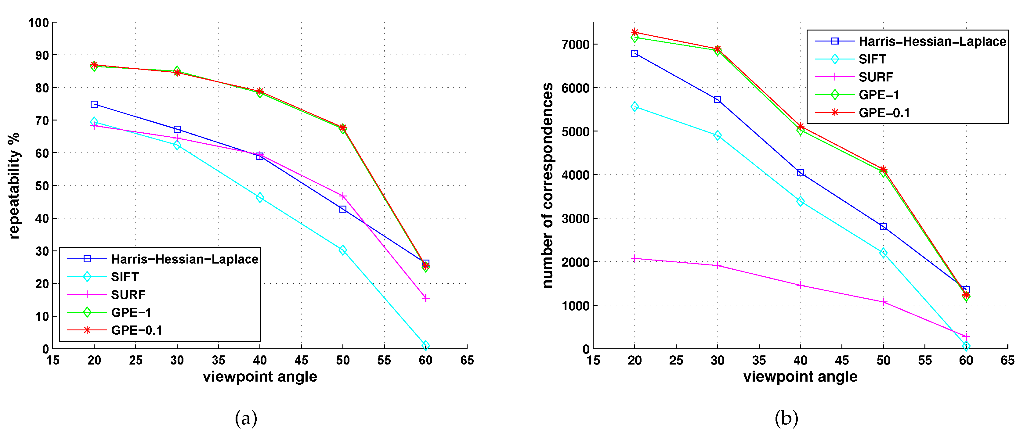
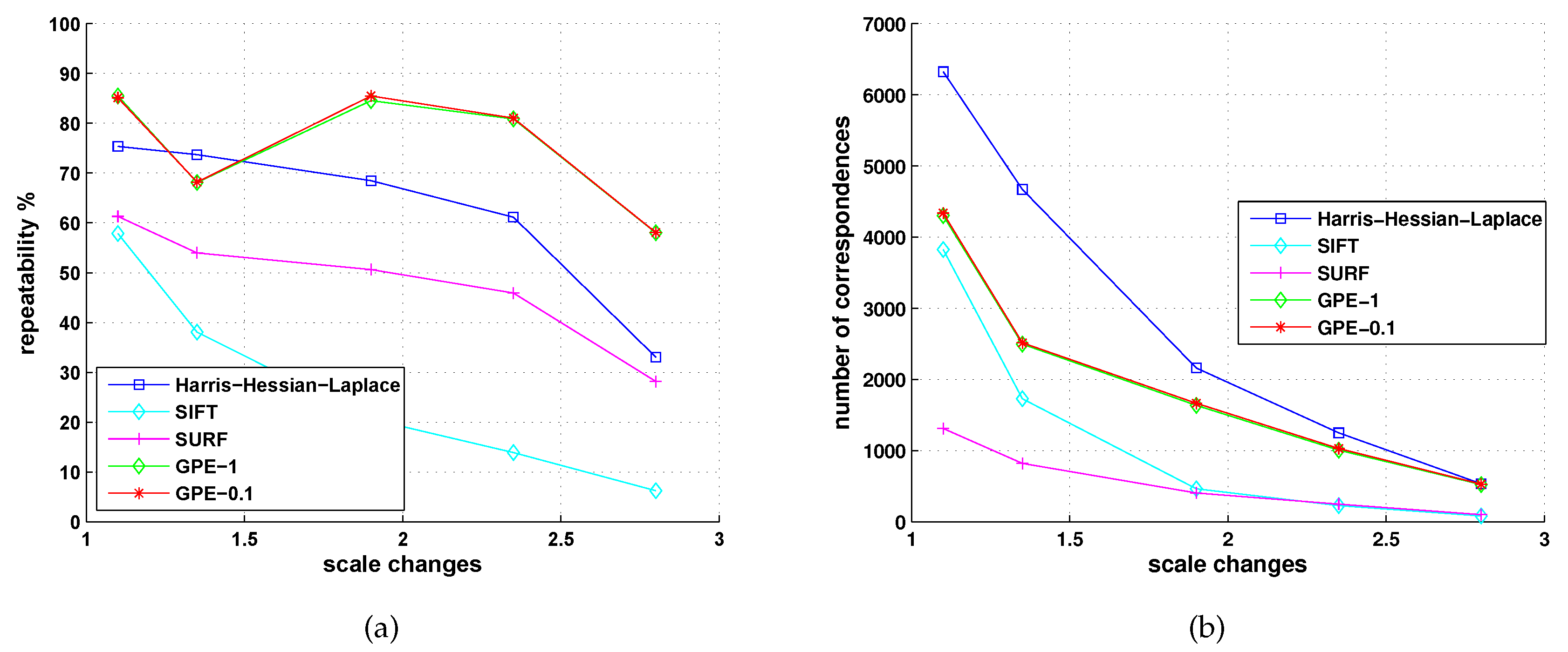
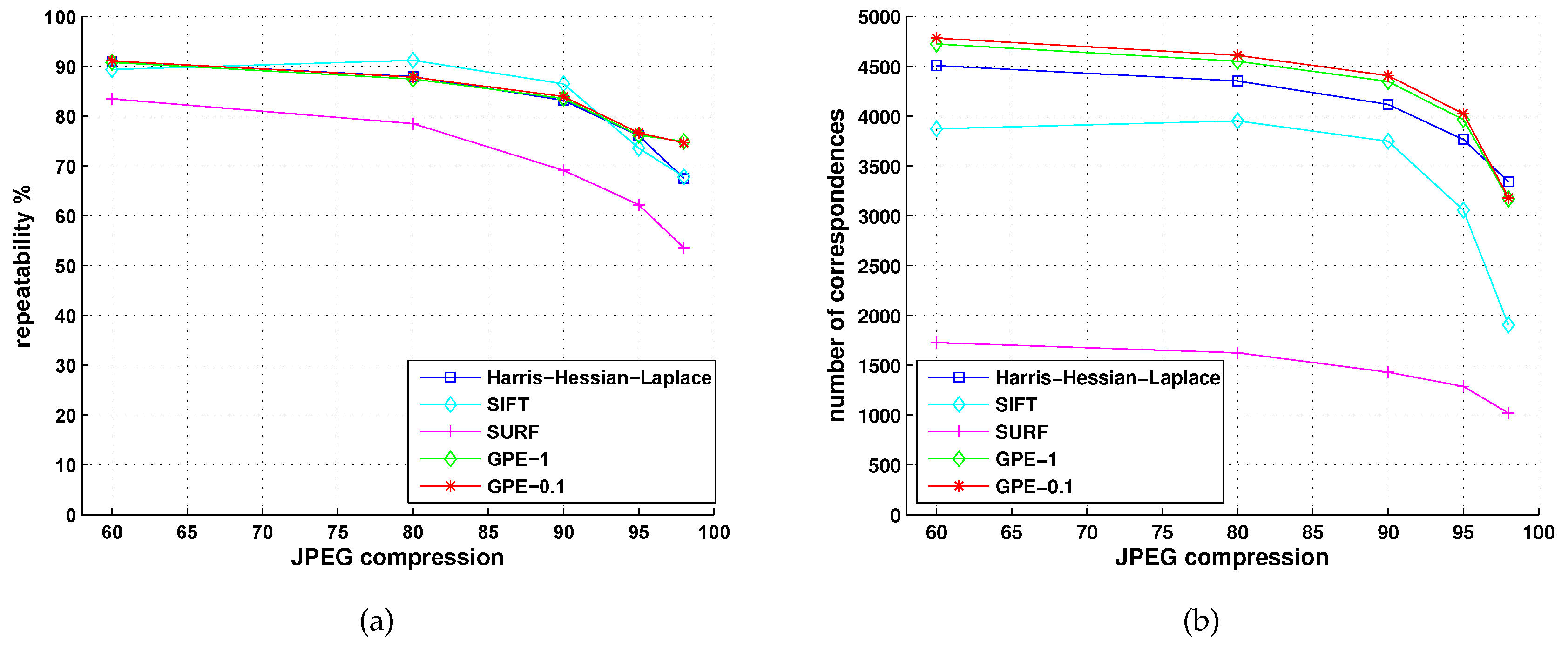
5.1. Comparison with Affine Detectors

In the work [13], there are eight sets of test results for six affine region detectors, namely Harris-Affine [8,14,15], Hessian-Affine [8,14], MSER [16], IBR [15,17], EBR [17,18], and Salient [19].
Since GPE is not intended for the situation of viewpoint change, when the viewpoint angle is greater than 30 degrees, the repeatability score for structured scene is less than all those affine detectors. However, from 20 to 30 degrees, GPE drastically overcomes any other detectors (cf. Figures 1a and 13a in [13]). In the situation of the images containing repeated texture motifs, in Figure 2a (in comparison with Figure 14a in [13]), it can be seen that, except viewpoint change of 60 degrees, GPE reaches higher repeatability score than all affine detectors, which means that, as long as the viewpoint angle is less than 50 degrees, GPE has strong capacity of extracting affine features. In the tests for scale change and rotation, GPE shows its obvious advantages in both structured scene and texture scene except at scale 4 in the textured scene, where Hessian-Affine attains the repeatability of 70 % (cf. Figures 3a and 4a and Figures 15a and 16a in [13]). In the results shown in Figure 5 (in contrast to Figure 17a in [13]) and Figure 6 (in contrast to Figure 18a in [13]), GPE shows excellent capacity to cope with the situation of blur in both structured scene and texture scene. In those comparisons, none of other detectors achieve higher repeatability score than GPE at any test point. In the test of JPEG compression, GPE has similar performance compared with Harris-Affine and Hessian-Affine, but obviously outperforms other LPE detectors (cf. Figures 7a and 19a in [13]). The Hessian-Affine detector shows its slight advantage for JPEG compression change. Figures 8a and 20a in [13] show that GPE has good robustness to illumination change and overall higher repeatability score than other extractors.

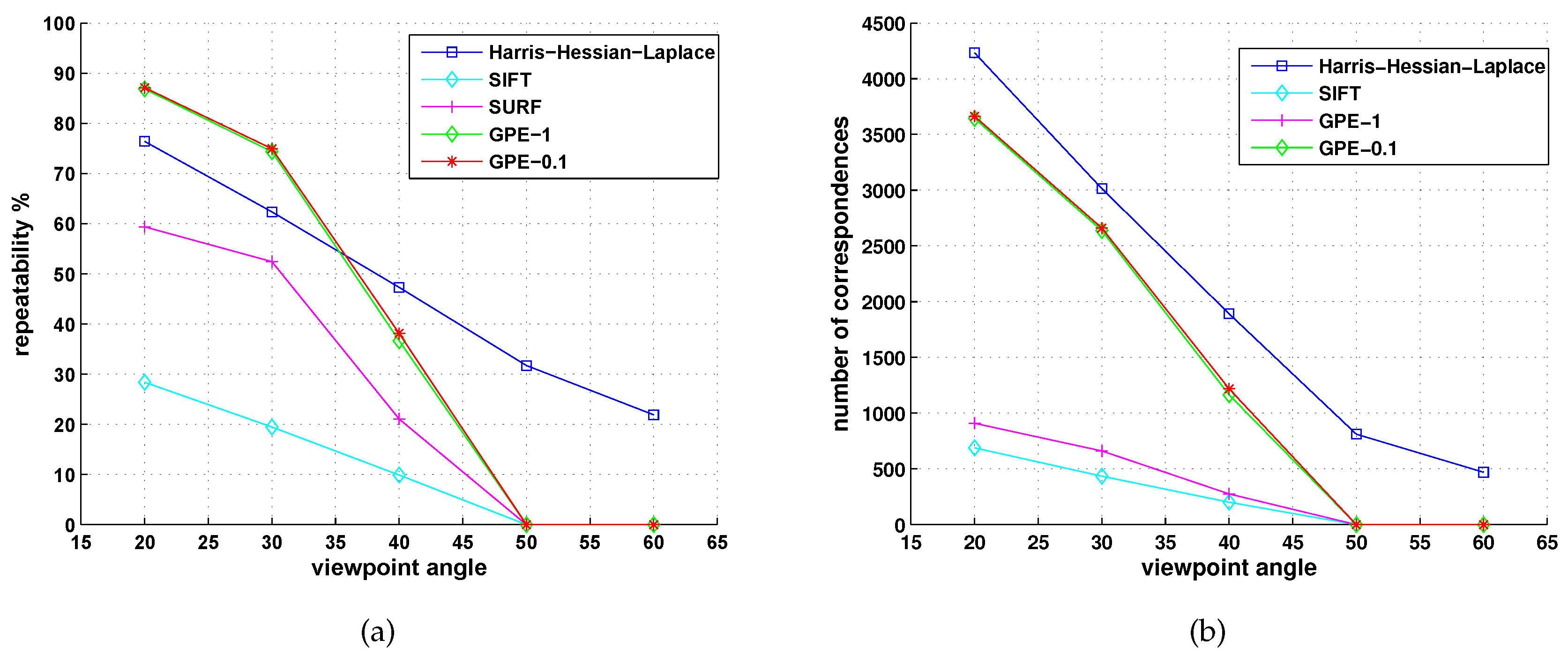
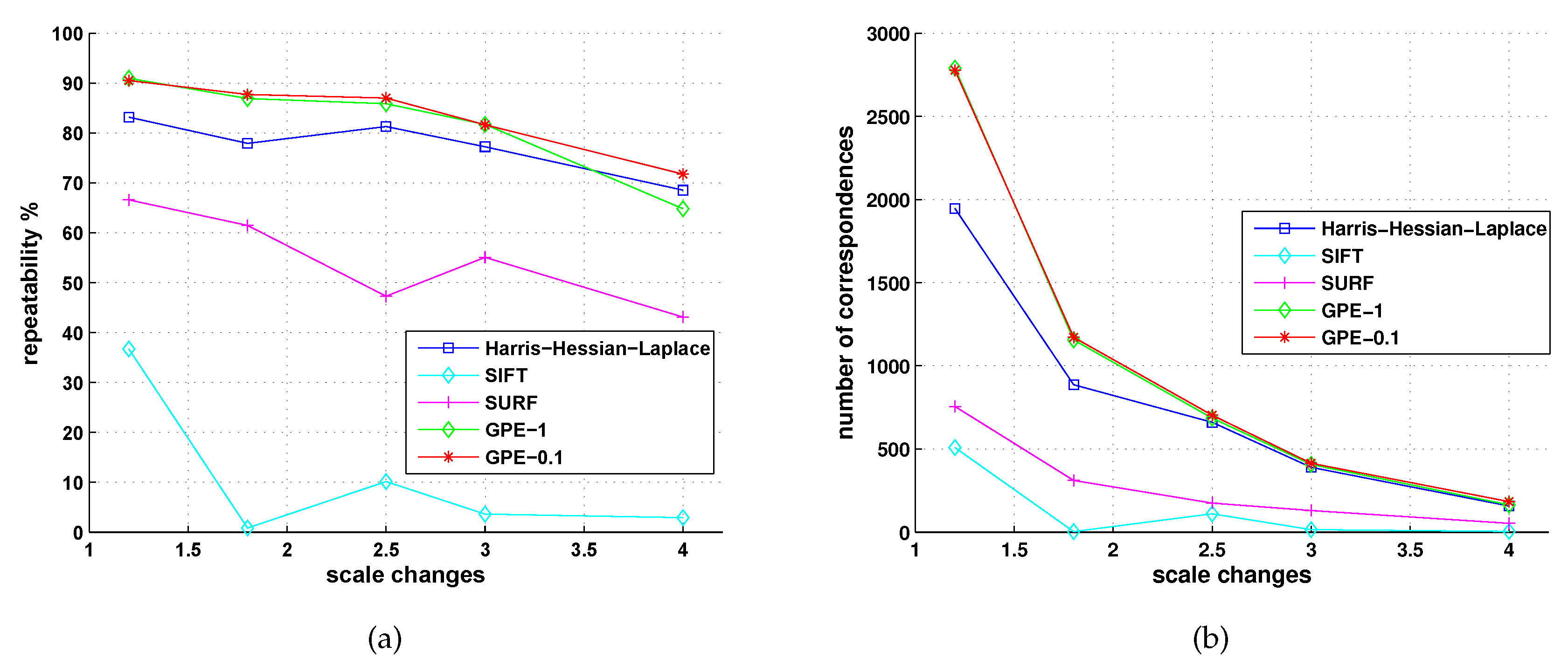
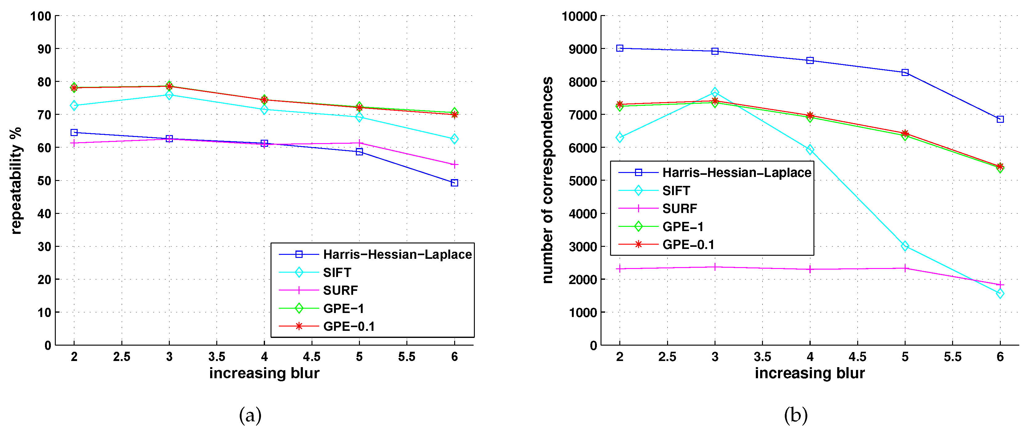
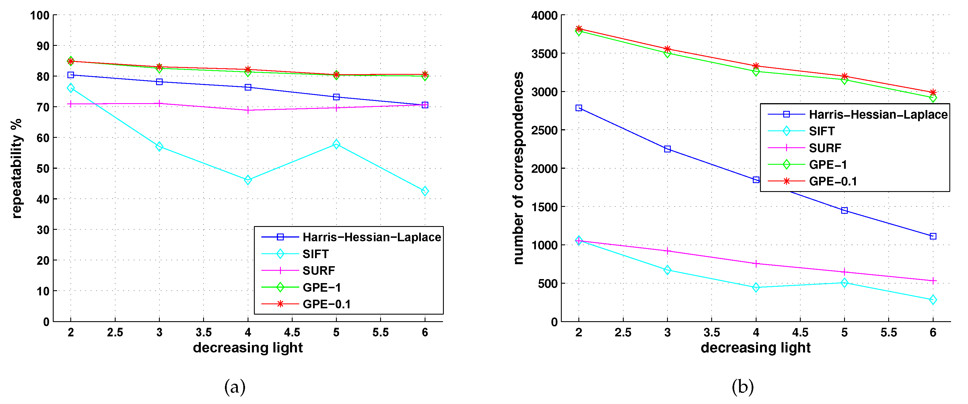
5.2. Comparison with Detectors of Fast-Hessian, DoG, Harris-Laplace and Hessian-Laplace

In the work [10], five detectors, FH-15, FH-9, DoG [6], Harris-Laplace, and Hessian-Laplace [14], were tested for repeatability performance of viewpoint change for structured scene, viewpoint change for textured scene, scale change for structured scene, and blur for structured scene. Therefore, there are four results can be adapted directly, which are shown in the Figures 16 and 17 in [10]. Comparing these results, respectively, with the (a) in Figure 1, Figure 2, Figure 3, Figure 4 and Figure 5, it can be seen that except one point (which is the scale change about 1.3 for FH-15 and DoG), GPE apparently overcomes FH-15, FH-9, DoG, Harris-Laplace, and Hessian-Laplace in all these tests.

5.3. Comparison with Locally Contrasting Keypoints Detector

Figure 5 in [11] and Figure 7 in [12] show results in the tests of LOCKY, where the sub-figures, (a)–(h) correspond to Figure 1a, Figure 2a, Figure 3a, Figure 4a, Figure 5a, Figure 6a, Figure 7 and Figure 8a, respectively, in our work. Since LOCKY mainly aims to achieve faster computation than most of the currently used feature detectors, except the cases that viewpoints are greater than 40 in the Graffiti sequence, GPE shows apparently higher repeatability score than LOCKY.

6. Conclusions

We present a new method (GPE) for local feature extracting with high repeatability, which transforms a discretized scale-space presentation through LoG and extracts local features by the scheme of global comparison. Because convolution templates of disk shape are used, GPE is rotation-invariant. Discussion for the radii of convolution templates and the error caused by finite radii is an important merit in our work. We first decompose the LoG transformation of a discretized scale-space presentation into two parts, the approximation and the error. Then, an upper bound of the error under a given radius is worked out and we utilize this upper bound to determinate a threshold, below which the candidates are no longer regarded as features since the computational error can influence the precision of the approximation (cf. Equations (6) and (7)). Because of the global comparison, the relative threshold can be employed to choose local features from candidates, and hence these chosen features are illumination-invariant. Since the kernel width increases only one pixel a time, GPE obtains more precise scales for extracted local features without interpolation than LPE does, and therefore the step of interpolation for precisely locating the scale of a feature point in LPE is elided in GPE. Simulations show that GPE reaches high performance for repeatability and true recalls in various situations, including scale change, rotation, blur, JPEG compression, illumination change, and even viewpoint change of a textured scene.

Author Contributions

Methodology, original draft and writing, Q.Z.; Supervision, B.S.

Funding

This research was supported by Guangdong Project of Science and Technology Development (2014B09091042) and Guangzhou Sci & Tech Innovation Committee (201707010068).

Acknowledgments

The authors appreciate Krystian Mikolajczyk for his test dataset, criteria and executable files. The authors are also thankful to David Lowe for his executable file of SIFT, and to Chris Evan for his code of OpenSURF.

Conflicts of Interest

The authors declare no conflict of interest.

References

  1. Harris, C.; Stephens, M. A combined corner and edge detector. Proc. Alvey Vision Conf. 1988, 1988, 147–151. [Google Scholar]
  2. Dufournaud, Y.; Schmid, C.; Horaud, R. Matching images with different resolutions. In Proceedings of the IEEE Conference on Computer Vision and Pattern Recognition, Hilton Head Island, SC, USA, 15 June 2000; Volume 1, pp. 612–618. [Google Scholar] [CrossRef]
  3. Lindeberg, T. Feature Detection with Automatic Scale Selection. Int. J. Comput. Vis. 1998, 30, 79–116. [Google Scholar] [CrossRef]
  4. Lindeberg, T. Scale-space theory: A basic tool for analyzing structures at different scales. J. Appl. Stat. 1994, 21, 225–270. [Google Scholar] [CrossRef]
  5. Lowe, D.G. Object recognition from local scale-invariant features. iccv 1999, 2, 1150–1157. [Google Scholar] [CrossRef]
  6. Lowe, D.G. Distinctive Image Features from Scale-Invariant Keypoints. Int. J. Comput. Vis. 2004, 60, 91–110. [Google Scholar] [CrossRef]
  7. Mikolajczyk, K.; Schmid, C. Indexing based on scale invariant interest points. In Proceedings of the Eighth IEEE International Conference on Computer Vision (ICCV 2001), Vancouver, BC, Canada, July 7–14 2001; Volume 1, pp. 525–531. [Google Scholar] [CrossRef]
  8. Mikolajczyk, K.; Schmid, C. An Affine Invariant Interest Point Detector. In Computer Vision—ECCV 2002: 7th European Conference on Computer Vision Copenhagen, Denmark, May 28–31, 2002 Proceedings, Part I; Heyden, A., Sparr, G., Nielsen, M., Johansen, P., Eds.; Springer: Berlin/Heidelberg, Germany, 2002; pp. 128–142. [Google Scholar] [CrossRef]
  9. Bay, H.; Tuytelaars, T.; Van Gool, L. SURF: Speeded Up Robust Features. In Computer Vision—ECCV 2006: 9th European Conference on Computer Vision, Graz, Austria, May 7–13, 2006. Proceedings, Part I; Leonardis, A., Bischof, H., Pinz, A., Eds.; Springer: Berlin/Heidelberg, Germany, 2006; pp. 404–417. [Google Scholar] [CrossRef]
  10. Bay, H.; Ess, A.; Tuytelaars, T.; Gool, L.V. Speeded-Up Robust Features (SURF). Comput. Vis. Image Underst. 2008, 110, 346–359. [Google Scholar] [CrossRef]
  11. Lomeli-R, J.; Nixon, M.S. The Brightness Clustering Transform and Locally Contrasting Keypoints. In Computer Analysis of Images and Patterns; Azzopardi, G., Petkov, N., Eds.; Springer International Publishing: Cham, Switzerland, 2015; pp. 362–373. [Google Scholar]
  12. Lomeli-R, J.; Nixon, M.S. An extension to the brightness clustering transform and locally contrasting keypoints. Mach. Vis. Appl. 2016, 27, 1187–1196. [Google Scholar] [CrossRef]
  13. Mikolajczyk, K.; Tuytelaars, T.; Schmid, C.; Zisserman, A.; Matas, J.; Schaffalitzky, F.; Kadir, T.; Gool, L.V. A Comparison of Affine Region Detectors. Int. J. Comput. Vis. 2005, 65, 43–72. [Google Scholar] [CrossRef]
  14. Mikolajczyk, K.; Schmid, C. Scale & Affine Invariant Interest Point Detectors. Int. J. Comput. Vis. 2004, 60, 63–86. [Google Scholar] [CrossRef]
  15. Schaffalitzky, F.; Zisserman, A. Multi-view Matching for Unordered Image Sets, or “How Do I Organize My Holiday Snaps?”. In Computer Vision—ECCV 2002: 7th European Conference on Computer Vision Copenhagen, Denmark, May 28–31, 2002 Proceedings, Part I; Heyden, A., Sparr, G., Nielsen, M., Johansen, P., Eds.; Springer: Berlin/Heidelberg, Germany, 2002; pp. 414–431. [Google Scholar] [CrossRef]
  16. Matas, J.; Chum, O.; Urban, M.; Pajdla, T. Robust Wide Baseline Stereo from Maximally Stable Extremal Regions. Br. Mach. Vis. Conf. 2002, 22, 384–393. [Google Scholar]
  17. Tuytelaars, T.; Gool, L.V. Wide baseline stereo matching based on local, affinely invariant regions. In Proceedings of the British Machine Vision Conference 2000 (BMVC 2000), Bristol, UK, 11–14 September 2000; pp. 412–425. [Google Scholar]
  18. Tuytelaars, T.; Van Gool, L. Matching Widely Separated Views Based on Affine Invariant Regions. Int. J. Comput. Vis. 2004, 59, 61–85. [Google Scholar] [CrossRef]
  19. Kadir, T.; Zisserman, A.; Brady, M. An Affine Invariant Salient Region Detector. In European Conference on Computer Vision; Springer: Berlin/Heidelberg, Germany, 2004; pp. 228–241. [Google Scholar]
Figure 1. Repeatability score (a) and number of correspondences (b) under viewpoint change for the structured scene by the Graffiti sequence.
Information 10 00376 g001
Figure 2. Repeatability score (a) and number of correspondences (b) under viewpoint change for the textured scene by the Wall sequence.
Information 10 00376 g002
Figure 3. Repeatability score (a) and number of correspondences (b) under scale change for the structured scene by the Boat sequence.
Information 10 00376 g003
Figure 4. Repeatability score (a) and number of correspondences (b) under scale change for the textured scene by the Bark sequence.
Information 10 00376 g004
Figure 5. Repeatability score (a) and number of correspondences (b) under blur for the structured scene by the Bikes sequence.
Information 10 00376 g005
Figure 6. Repeatability score (a) and number of correspondences (b) under blur for the textured scene by the Trees sequence.
Information 10 00376 g006
Figure 7. Repeatability score (a) and number of correspondences (b) under JPEG compression by the UBC sequence.
Information 10 00376 g007
Figure 8. Repeatability score (a) and number of correspondences (b) under illumination change by the Leuven sequence.
Information 10 00376 g008

