Decision Diagram Algorithms to Extract Minimal Cutsets of Finite Degradation Models

Abstract

In this article, we propose decision diagram algorithms to extract minimal cutsets of finite degradation models. Finite degradation models generalize and unify combinatorial models used to support probabilistic risk, reliability and safety analyses (fault trees, attack trees, reliability block diagrams…). They formalize a key idea underlying all risk assessment methods: states of the models represent levels of degradation of the system under study. Although these states cannot be totally ordered, they have a rich algebraic structure that can be exploited to extract minimal cutsets of models, which represent the most relevant scenarios of failure. The notion of minimal cutsets we introduce here generalizes the one defined for fault trees. We show how algorithms used to calculate minimal cutsets can be lifted up to finite degradation models, thanks to a generic decomposition theorem and an extension of the binary decision diagrams technology. We discuss the implementation and performance issues. Finally, we illustrate the interest of the proposed technology by means of the use case stemmed from the oil and gas industry.

1. Introduction

Since the famous WASH report [1] that followed the Three Mile Island nuclear accident, probabilistic risk, reliability and safety analyses have been developed considerably. They are nowadays applied to virtually all industrial systems the operation of which presents a risk for the systems themselves, their operators or their environment.

Probabilistic risk, reliability and safety assessment models describe how a system may degrade and eventually fail under the occurrence of random events such as failures of mechanical components, sudden changes in environmental conditions or human errors. They can be split into three nested categories: combinatorial models, state automata and process algebras [2].

Combinatorial models are the simplest, but also by far the most widely used. In these models, the state of the system is described as a combination of the states of its components. As the number of possible states considered for each component is finite, and in general small, the number of possible states of the system is also finite, although subject to an exponential blow-up. Boolean models, i.e., fault trees, reliability block diagrams and event trees, belong to this category, see e.g., [3,4] for reference textbooks. So-called multistate systems [5,6,7], i.e., extensions of Boolean models to the case where components can be in more than two—but still a finite number of—states, enter also in this category.

Intuitively, combinatorial models take a snapshot of the system at a given point in time. They do not consider the trajectory that lead the system from its initial state to its current state. Consequently, they can only approximate time dependencies induced for instance by cold-redundancies or reconfigurations. To take into account such dependencies, one needs more expressive models such as Markov chains [8], stochastic Petri nets [9], or guarded transition systems [10,11]. These models enter either in the category of state automata or in the category of process algebras. However, the more expressive the model, the more computationally expensive the calculation of probabilistic indicators from that model. Consequently, probabilistic risk, reliability and safety assessment models result always of a tradeoff between the accuracy of the description of the system under study and the ability to perform calculations on this description, see reference [2] for an in-depth discussion. Moreover, the more expressive the model, the harder it is to design, to validate and to maintain. This is the reason why combinatorial models, and more specifically Boolean models, dominate the industrial practice.

It remains that, with the steadily increasing complexity of technical systems, the more expressive power we can have for the models, the better, with the proviso that the added expressive power does not degrade the computational complexity of assessments. This is why lots of efforts have been made in the recent years on the study of multistate systems. This is also what led us to introduce the algebraic concept of finite degradation structures [12]. Finite degradation models generalize and unify both Boolean models and multistate systems. They can be seen as the most general mathematical framework that can be used to design probabilistic risk assessment models, while staying in the realm of combinatorial models.

Calculations performed on Boolean models belong formally to two distinct categories: qualitative assessments and quantitative assessments. The former aim primarily at extracting and classifying minimal cutsets. Minimal cutsets represent minimal scenarios of failure. The latter aim primarily at calculating probabilistic risk indicators such as the unavailability of the system (probability that the system is failed at time t), safety integrity levels or importance measures. In practice, this distinction is blurred because there are so many minimal cutsets that only the most relevant, i.e., the most probable, ones can be extracted. Moreover, the best way of calculating probabilistic indicators is to assess them via minimal cutsets. This is the reason why the extraction of the most probable minimal cutsets plays a central role in probabilistic risk and safety analyses.

Finite degradation structures formalize what is probably the most fundamental idea underlying all risk assessment methods: the states of a model represent essentially various levels of degradation of the system under study. Although these states cannot be totally ordered, they have rich algebraic structure that can be exploited both by analysts and by assessment algorithms: when studying a given level of degradation of the system, one is interested in the minimal conditions that produce this degradation level. These conditions are in turn characterized by the minimal states, according to the degradation order, in which the system is in the given degradation level. In other words, the notion of minimal cutset, or minimal state, of finite degradation models generalizes and sheds a new light on the one defined for fault trees.

There are essentially two families of algorithms to extract minimal cutsets. The first one consists of top-down algorithms. MOCUS [13] and its modern versions such as the one implemented in RiskSpectrum [14] and the one implemented in XFTA [15], belong to this family. The second family consists of bottom-up algorithms based on the binary decision diagrams technology [16,17,18]. We show here how to extend this technology so to handle finite degradation structures, via ideas introduced by Minato [19] (in a different context). For this purpose, we introduce the notion of implicative normal form for formulas encoding discrete functions. We demonstrate a generic decomposition theorem making it possible the extraction of the most probable minimal states. This theorem generalizes the one of reference [16], which is at core of minimal cutsets calculations.

The contribution of this article is thus fourfold. First, it shows how to generalize the concept of minimal cutsets to finite degradation models. Second, it demonstrates a decomposition theorem that makes possible to lift-up Boolean algorithms proposed in reference [16] to finite degradation models. Third, it shows how to extend the binary decision diagram technology so to handle finite degradation models. Last, it discusses approximation schemes in the context of finite degradation models.

The remainder of this article is organized as follows. Section 2 presents an illustrative example stemmed from the oil and gas industry. Section 3 introduces finite degradation structures and finite degradation models. Section 4 shows how to lift-up the notion of minimal cutset. Section 5 shows how to extend the binary decision diagrams technology. Section 6 discusses approximation schemes. Section 7 provides some experimental results. Finally, Section 8 concludes the article.

Appendix A presents the full model of the use case.

2. Illustrative Example

This section presents an example we shall use throughout the article to illustrate the proposed approach.

2.1. Description

The high pressure protection system pictured in Figure 1 is referred to as TA4 in ISO/TR 12489 standard [20].

The objective of this safety instrumented system is to protect a pipe section from overpressures. It involves seven main components: three sensors (S1, S2 and S3), two logic solvers (LS1 and LS2) and two actuators (the isolation valves V1 and V2). When the sensors detect an overpressure in the protected section, the logic solvers order the isolation valves to close so to release the pressure. The logic solver LS2 works according to a 1-out-of-2 logic, i.e., that it sends the order to close the valves if at least one out of two sensors S2 and S3 detects an overpressure.

As the failure of the TA4 HIPPS may result in a catastrophic accident, it is of importance to assess its reliability. This is classically done by means of a fault tree such as the one pictured in Figure 2.

2.2. Classification of Failures

The fault tree pictured in Figure 2 does not distinguish however the different types of failures. According to the standard IEC61508 [21], individual failures of components and global failures of a safety instrumented system can be classified along two directions: safe versus dangerous failures, and detected versus undetected failures. One finds similar classifications in other safety standards such as ISO 26262 [22].

In our example, safe failures are those which contribute to close the isolation valves, even though there is no overpressure (spurious triggers), while dangerous failures are those which contribute to keep the isolation valves open, even though there is an overpressure. These two types of failures have indeed very different consequences: the former hampers the profitability of the production while the latter may result in catastrophic accidents. Moreover, their frequencies may be very different.

If we look more specifically at dangerous failures, we need to distinguish detected and undetected ones. Logic solvers embed autotest facilities so that their failures are immediately detected. On the contrary, failure of valves remain undetected between two maintenance interventions. Failures of sensors may be detected or not.

ISO/TR 12489 makes the additional following assumptions.

• All other components may fail (independently). Their probabilities of failure follow negative exponential distributions. The parameters of these distributions are given in

  Table 1. TA4 reliability parameters.

  Parameter	Sensor	Logic Solver	Isolation Valve
  Safe failure rate	3.00 × 10−6 h${}^{-1}$	3.00 × 10−7 h${}^{-1}$	NA
  Dangerous detected failure rate	3.00 × 10−7 h${}^{-1}$	6.00 × 10−7 h${}^{-1}$	2.90 × 10−6 h${}^{-1}$
  Dangerous undetected failure rate	3.00 × 10−7 h${}^{-1}$	NA	2.90 × 10−7 h${}^{-1}$

  . Safe failures are always detected.
• The system is maintained once a year (once in 8760 hours). The production is stopped during the maintenance. Components are as good as new after the maintenance.

2.3. Discussion

The Boolean logic at work in fault trees and related formalisms does not make it possible to distinguish the different types of failures. More exactly, it would be possible to design a fault tree for each type of failure, but this would be both tedious and error prone. Hence the idea to use multi-valued logics, in which variables and formulas can take more than two, but still a finite number of values [7]. This raises however two conceptual and practical issues:

• Which algebraic properties such a logic should they obey so that usual notions of reliability engineering (minimal cutsets, top-event probability, importance measures, safety integrity levels…) can be lifted-up into the logic?
• Once the mathematical foundations have been established, how to perform efficiently calculations of risk indicators?

Finite degradation structures provide a general mathematical framework to answer the first question. In this article, we provide a concrete answer to the second one.

3. Finite Degradation Models

This section introduces finite degradation models which unify and generalize the various types of combinatorial models used in the framework of probabilistic risk, reliability and safety analyses.

3.1. Finite Degradation Structures

A finite degradation structure is a triple $\langle C,{\le }_C,{\perp }_C\rangle$ where:

• C is a finite set of constants.
• ${\le }_C$ is a partial order over C.
• ${\perp }_C$ is the unique lower bound of C, i.e., the unique element such that ${\perp }_C{\le }_{C}x$ for all $x\in C$.

Technically, finite degradation structures are thus semi-lattices. C is called the support set of the finite degradation structure.

The idea behind finite degradation structures is that each element of C represents a possible state of the system under study. The partial order ${\le }_C$ sorts states according to their level of degradation, i.e., $s{\le }_{C}t$ if the system is less degraded in the state s than in the state t. Finally, ${\perp }_C$ represents the initial, nominal state of the system.

Figure 3 shows Hasse diagrams representing some typical finite degradation structures. In these diagrams, the degradation order is represented bottom-up.

The finite degradation structure $\mathbf{WF}$ is the classical Boolean domain: w and f stand respectively for working and failed. Indeed, f is more degraded than w. The finite degradation structure $\mathbf{WDF}$ introduces the intermediate value d, which stands for degraded. Hence the natural degradation order $\mathtt{w}<\mathtt{d}<\mathtt{f}$. In the finite degradation structure $\mathbf{WFsd}$, the failure state fs (failed safe) is not comparable with the failure state fd (failed dangerous) although both are more degraded than the working state w. The finite degradation structure $\mathbf{WFdu}$ distinguishes two types of dangerous failures: detected ones (fd) and undetected ones (fu). Of course, undetected failures are more problematic than detected ones. Hence the order $\mathtt{w}<\mathtt{fd}<\mathtt{fu}$. Last but not least, the finite degradation structure $\mathbf{W}\mathbf{3}\mathbf{F}$ combines $\mathbf{WFsd}$ and $\mathbf{WFsd}$. We shall come back on this finite degradation structure that is, implicitly, at the core of safety standards such as IEC61508 [21] and ISO/TR 12489 [20].

Note that $\mathbf{WDF}$ and $\mathbf{WFdu}$ are isomorphic. However, operations on these two finite degradation structures are different. It is thus worth to consider them as distinct.

3.2. Product

Now, let $\mathcal{C}:\langle C,{\le }_C,{\perp }_C\rangle$ and $\mathcal{D}:\langle D,{\le }_D,{\perp }_D\rangle$ be two finite degradation structures, the product of $\mathcal{C}$ and $\mathcal{D}$, denoted by $\mathcal{C}\otimes \mathcal{D}$, is the triple $\langle C\times D,{\le }_{C\times D},{\perp }_{C\times D}\rangle$, where:

• $C\times D$ stands for the Cartesian product of C and D.
• For all $x,x^{\prime }\in C$ and $y,y^{\prime }\in D$, $\langle x,y\rangle {\le }_{C\times D}\langle x^{\prime },y^{\prime }\rangle$ if and only if $x{\le }_C{x}^{\prime }$ and $y{\le }_D{y}^{\prime }$.
• ${\perp }_{C\times D}=\langle {\perp }_C,{\perp }_D\rangle$.

It is easy to verify that $\mathcal{C}\otimes \mathcal{D}$ is a finite degradation structure. This is by no means surprising as the category of partial orders has a product [23].

The product ⊗ is commutative and associative up to an isomorphism, i.e., $\mathcal{C}\otimes \mathcal{D}\cong \mathcal{D}\otimes \mathcal{C}$ and $\mathcal{C}\otimes (\mathcal{D}\otimes \mathcal{E})\cong (\mathcal{C}\otimes \mathcal{D})\otimes \mathcal{E}$ for all finite degradation structures $\mathcal{C}$, $\mathcal{D}$ and $\mathcal{E}$. The finite degradation structure $\mathbf{1}=\langle \{\perp \},\perp \le \perp ,\perp \rangle$ is a neutral element for this product: $\mathbf{1}\otimes \mathcal{C}\cong \mathcal{C}\otimes \mathbf{1}\cong \mathcal{C}$ for any finite degradation structure $\mathcal{C}$.

The existence of a product over finite degradation structures makes it possible to describe the state of system as the combination of the states of its components.

Consider, for instance, a system made of two components A and B. Assume that both A and B are represented by means of the finite degradation structure $\mathbf{WDF}$. Then, the state space of the system is represented by the finite degradation structure ${\mathbf{WDF}}^2$ pictured in Figure 4.

Note that although $\mathbf{WDF}$ encodes a total order over its elements, ${\mathbf{WDF}}^2$ encodes only a partial order.

3.3. Formulas

In the previous example, the state of the system is represented by a pair. Now if, for instance, the components A and B are in series, we can map each pair onto an element of $\mathbf{WDF}$, e.g. $(\mathtt{w},\mathtt{w})$ is mapped onto $\mathtt{w}$, $(\mathtt{w},\mathtt{d})$ is mapped onto $\mathtt{d}$, $(\mathtt{w},\mathtt{f})$ is mapped onto $\mathtt{f}$, and so on. There are indeed several ways to define such a mapping. Moreover the target finite degradation structure does not need to be the same as the source ones, which themselves may differ one another. In other words, it is possible to define a collection of operators on finite degradation structures.

In the sequel, we shall thus assume a finite set $\mathcal{U}$ of finite degradation structures and a finite set $\mathcal{O}$ of symbols called operators.

Each operator o of $\mathcal{O}$ is associated with a mapping $⟦o⟧$ from ${⨂}_{1\le i\le n}{s}_i$, $n\ge 0$, into s, where both the $s_i$’s and s are finite degradation structures. n is the arity of o. ${⨂}_{1\le i\le n}{s}_i$ is called the domain of o and is denoted $dom(o)$. s is called the codomain of o and is denoted $codom(o)$. The signature of o, which characterizes its arguments and return types, is denoted ${⨂}_{1\le i\le n}{s}_i\to s$.

It is often, but not always, the case that operators are abstractions. Abstractions are surjective structure preserving mappings, i.e., an abstraction $\alpha :{⨂}_{1\le i\le n}{s}_i\to s$ obeys the following conditions:

• For all $\overline{u},\overline{v}\in {⨂}_{1\le i\le n}{s}_i$, $\overline{u}\le \overline{v}\Rightarrow \alpha (\overline{u})\le \alpha (\overline{v})$.
• $\alpha ({⨂}_{1\le i\le n}{\perp }_{s_i})={\perp }_s$.
• $\forall v\in s,\exists \overline{u}\in {⨂}_{1\le i\le n}{s}_i$ such that $\alpha (\overline{u})=v$.

As abstractions are epimorphisms in the sense of category theory, we shall use in the sequel the usual symbol ↠ for their signature, i.e., ${⨂}_{1\le i\le n}{s}_i\twoheadrightarrow s$.

It is easy to check that the notion of abstraction generalizes the notion of monotone Boolean function.

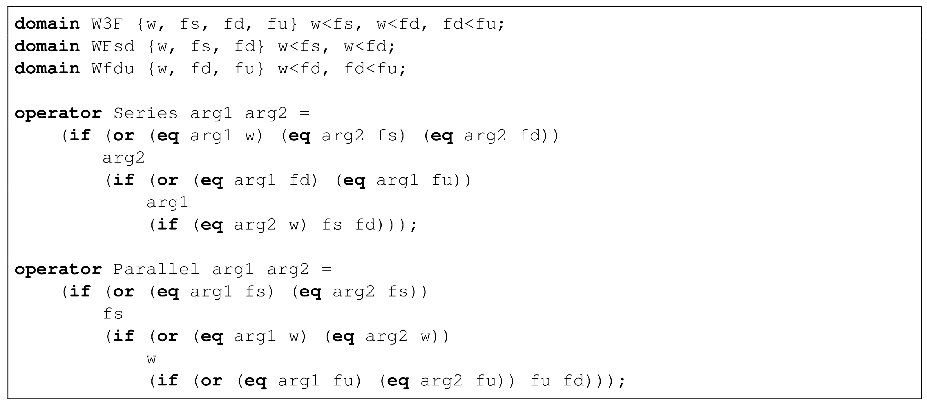
As an illustration, one can consider the two binary operators ⧁ and ‖ from $\mathbf{W}\mathbf{3}\mathbf{F}\otimes \mathbf{W}\mathbf{3}\mathbf{F}$ into $\mathbf{W}\mathbf{3}\mathbf{F}$. The operator ⧁ represents the series composition. It generalizes the Boolean operator ∨ (or). The operator ‖ represents the parallel composition. It generalizes the Boolean operator ∧ (and). These operators are defined in

Table 2. Definition of operators ⧁ and ‖.

$\mathit{U}⧁\mathit{V}$		V				$\mathit{U}\Vert \mathit{V}$		V
		w	fs	fd	fu			w	fs	fd	fu
U	w	w	fs	fd	fu	U	w	w	fs	w	w
	fs	fs	fs	fd	fd		fs	fs	fs	fs	fs
	fd	fd	fs	fd	fd		fd	w	fs	fd	fu
	fu	fu	fs	fd	fu		fu	w	fs	fu	fu

.

It is easy to verify that the series operator ⧁ is not commutative but associative and that the parallel operator ‖ is both commutative and associative.

We can now define formulas of the finite degradation calculus.

Let $\mathcal{U}$ be a finite set of finite degradation structures, let $\mathcal{O}$ be a finite set of operators on $\mathcal{U}$ defined as above, and finally, let $\mathcal{V}$ be a finite set of symbols called variables. Each variable V of $\mathcal{V}$ is assumed to take its value in the support set of one of the finite degradation structures of $\mathcal{U}$. This finite degradation structure is called the domain of V and is denoted $dom(V)$.

The set of well formed (typed) formulas over $\mathcal{U}$, $\mathcal{V}$ and $\mathcal{O}$ is the smallest set such that:

• Constants, i.e., members of support sets of finite degradation structures of $\mathcal{U}$, are well formed formulas. The type of a constant is the finite degradation structure it comes from.
• Variables of $\mathcal{V}$ are well-formed formulas. The type of a variable V is simply its domain.
• If o is an operator of $\mathcal{O}$ such that $⟦o⟧:{⨂}_{1\le i\le n}{s}_i\to s$, and $f_1,\dots f_n$ are well formed formulas of types $s_1,\dots s_n$, then $o(f_1,\dots ,f_n)$ is a well formed formula of type s.

In the sequel, we shall say simply formula instead of a well-formed formula.

The set of variables occurring in the formula f is denoted $var(f)$.

A variable valuation of f is a mapping from $var(f)$ into ${\prod }_{V\in var(f)}dom(V)$, i.e., a function that associates with each variable a value of its domain.

f is interpreted as a mapping $⟦f⟧:{⨂}_{V\in var(f)}dom(V)\to s$ where s is the codomain of the outmost operator of f, by lifting up as usual variable valuations. Let $\sigma$ be a variable valuation of $var(f)$, then:

• If f is reduced to a constant c, then $⟦f⟧(\sigma )=c$.
• If f is reduced to a variable V, then $⟦f⟧(\sigma )=\sigma (V)$.
• If f is in the form $o(f_1,\dots ,f_n)$, then $⟦f⟧(\sigma )=⟦o⟧(⟦f_1⟧(\sigma ),\dots ,⟦f_n⟧(\sigma ))$.

3.4. Finite Degradation Models

Finite degradation models are obtained by lifting up fault tree constructions to the finite degradation calculus. Namely, a finite degradation model is a pair $\langle \mathcal{V}=\mathcal{S}\uplus \mathcal{F},\mathcal{E}\rangle$ where:

• $\mathcal{S}=\{V_1,\dots ,V_m\}$, $m\ge 1$, is a finite set of state variables.
• $\mathcal{F}=\{W_1,\dots ,W_n\}$, $n\ge 1$, is a finite set of flow variables.
• $\mathcal{E}=\{W_1:=f_1,\dots ,W_n:=f_n\}$ is a finite set of equations such that for $1\le j\le n$:

  –

  $W_j$ is the jth variable of $\mathcal{F}$.

  –

  $f_j$ is a formula built over $\mathcal{V}$.

  –

  $codom(f_j)=dom(W_j)$

We say that the flow variable $W_j$ depends on the (state or flow) variable V if either $V\in var(f_j)$ or there exists a variable $U\in var(f_j)$ that depends on V.

A finite degradation model is looped if one of its flow variable depends on itself. It is loop-free otherwise.

A finite degradation model is uniquely rooted if there is only one variable that occurs in no right member of an equation. Such a variable is a called the root of the model.

From now, we shall consider only well-typed, loop-free, uniquely rooted models.

It is easy to see that finite degradation models generalize fault trees: state and flow variables play respectively the roles of basic and internal events, while equations play the role of gates. Moreover, the root variable plays the role of the top event. The terms “state” and “flow” comes from guarded transition systems [10].

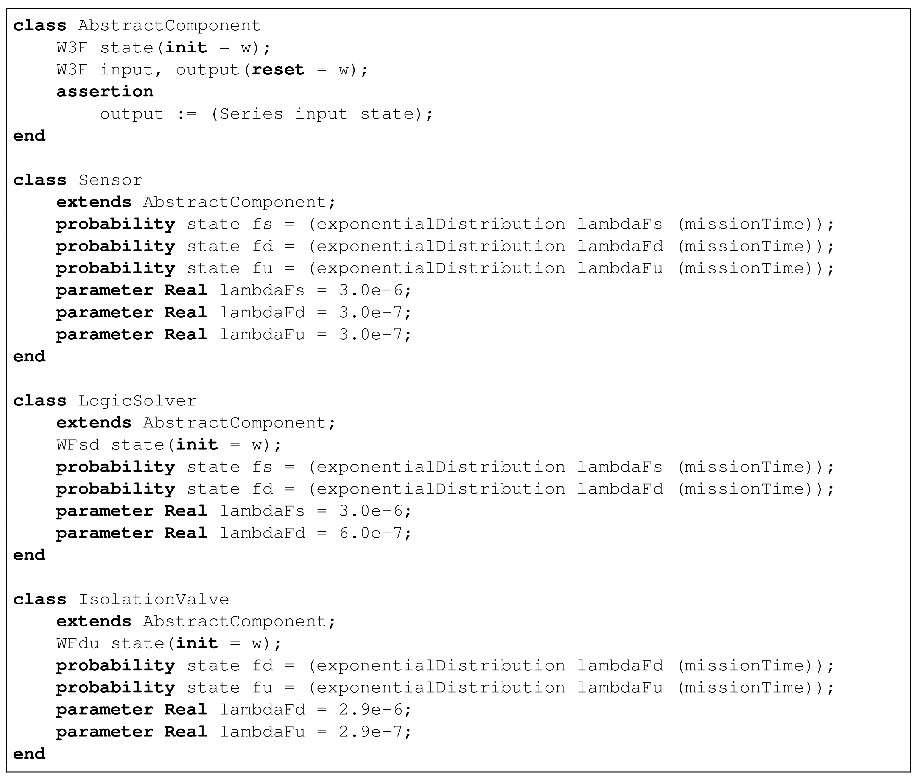
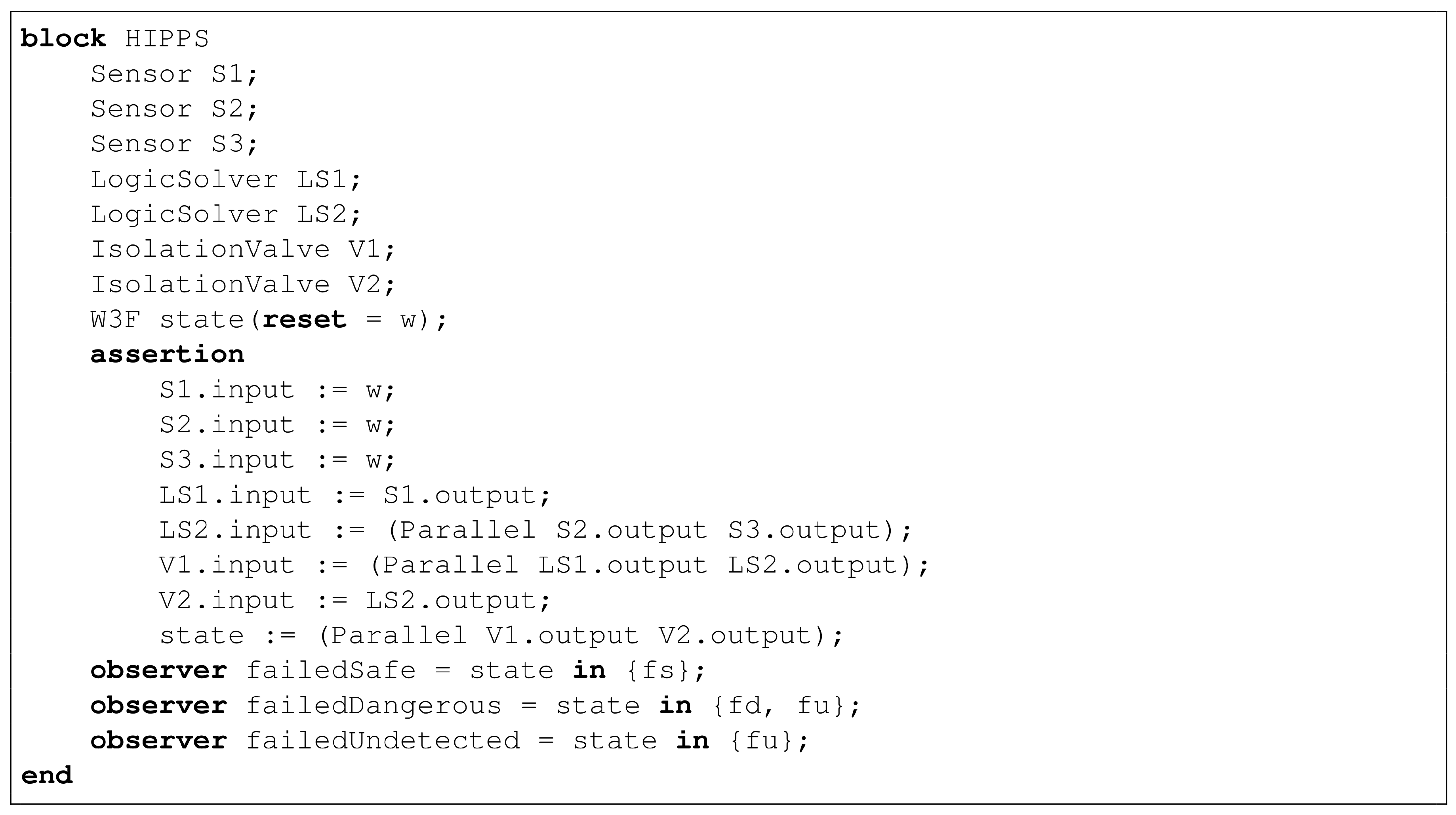
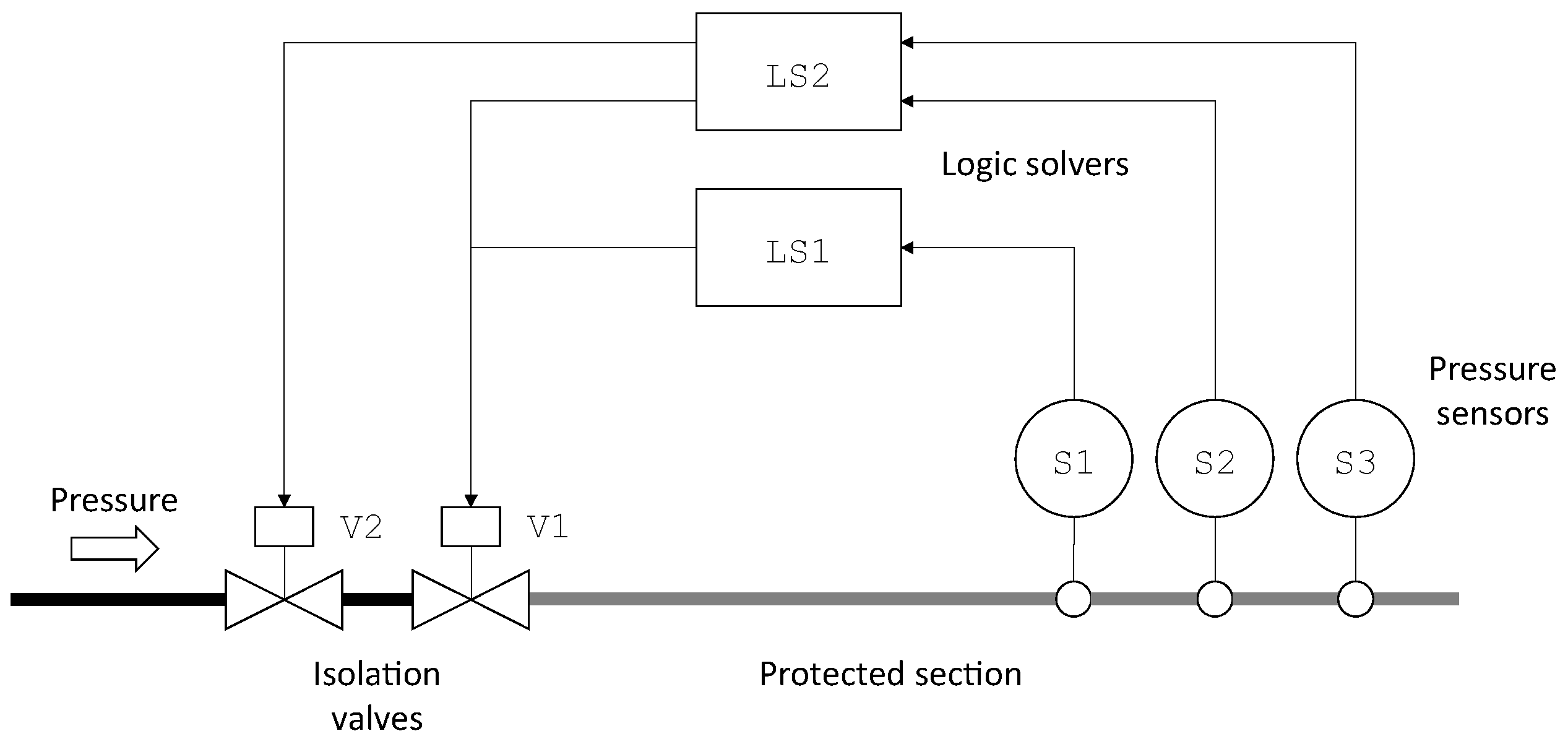
As an illustration, consider TA4 HIPPS presented Section 2. We can use the finite degradation structure W3F and the operators defined in Table 2 to represent this system.

The fault tree pictured in Figure 2 can be re-interpreted in this logic. Equations implementing this fault tree are given in

Table 3. Equations implementing the fault tree given in Table 2 in the $\mathbf{W}\mathbf{3}\mathbf{F}$ logic.

TA4	$:=$	SB1‖SB2
SB1	$:=$	S1⧁LS1⧁V1
SB2	$:=$	SL2⧁LS2⧁AL2
SL2	$:=$	S2‖S3
AL2	$:=$	V1‖V2

.

In this model, S1, S2, S3, LS1, LS2, V1 and V2 are state variables, while TA4, SB1, SB2, SL2 and AL2 are flow variables.

Note that LS1 and LS2 cannot take the value fu as we assumed that failures of logic solvers always detected. Similarly, V1 and V2 cannot take the value fs as we assumed that spurious closures of valves, if any, are immediately fixed.

3.5. Semantics

Let $\mathcal{M}:\langle \mathcal{V}=\mathcal{S}\uplus \mathcal{F},\mathcal{E}\rangle$ be a finite degradation model. A variable valuation of $\mathcal{V}$ is a function $\sigma :\mathcal{V}\to dom(\mathcal{V})$, i.e., a function that associates with each variable V of $\mathcal{V}$ a value in $dom(V)$.

A variable valuation $\sigma$ is admissible in the model $\mathcal{M}:\langle \mathcal{V},\mathcal{E}\rangle$ if $\sigma (W_j)=\sigma (f_j)$ for each equation $W_j:=f_j$ of $\mathcal{E}$.

The following property holds, thanks to the fact that the model is loop-free.

Lemma 1

(Unicity of admissible variable valuations). Let $\mathcal{M}$ be a finite degradation model and σ be a partial variable valuation that assigns values only to state variables of $\mathcal{M}$. Then there is a unique way to extend σ into an admissible total assigment ${\sigma }^{\prime }$ of variables of $\mathcal{M}$.

Note, ${\sigma }^{\prime }$ is simply calculated bottom-up by propagating values in equations.

In the sequel, we shall denote ${\stackrel{\rightharpoonup }{\sigma }}_{\mathcal{M}}$, or simply $\stackrel{\rightharpoonup }{\sigma }$ when the model $\mathcal{M}$ is clear from the context, this unique extension.

Consider for instance the model given in Table 3 and the valuation of state variables $\sigma :$$\mathtt{S}\mathtt{1}=\mathtt{w}$, $\mathtt{S}\mathtt{2}=\mathtt{fu}$, $\mathtt{S}\mathtt{3}=\mathtt{fd}$, $\mathtt{LS}\mathtt{1}=\mathtt{w}$, $\mathtt{LS}\mathtt{2}=\mathtt{w}$, $\mathtt{V}\mathtt{1}=\mathtt{fu}$ and $\mathtt{V}\mathtt{2}=\mathtt{w}$. Then, $\stackrel{\rightharpoonup }{\sigma }$ is the total variable valuation such that $\mathtt{SL}\mathtt{2}=\mathtt{fu}$, $\mathtt{AL}\mathtt{2}=\mathtt{w}$, $\mathtt{SB}\mathtt{1}=\mathtt{fu}$, $\mathtt{SB}\mathtt{2}=\mathtt{fu}$ and finally $\mathtt{TA}\mathtt{4}=\mathtt{fu}$.

There is indeed a one-to-one correspondence between variable valuations and elements of ${⨂}_{V\in \mathcal{V}}dom(V)$. We shall thus make no distinction between them in the sequel.

It follows from the above lemma, that we can interpret a model $\mathcal{M}:\langle \mathcal{V}=\mathcal{S}\uplus \mathcal{F},\mathcal{E}\rangle$ as a mapping:

$$⟦\mathcal{M}⟧:\underset{V\in \mathcal{S}}{⨂}dom(V)\to \underset{W\in \mathcal{F}}{⨂}dom(W)$$

Note that flow variables include in particular the root variable R of the model. Therefore, if we restrict $⟦\mathcal{M}⟧$ to its R component, we can interpret it as a mapping:

$${⟦\mathcal{M}⟧|}_R:\underset{V\in \mathcal{S}}{⨂}dom(V)\to dom(R)$$

This is indeed true for any other flow variable.

The following result holds.

Lemma 2

(Coherent finite degradation models). Let $\mathcal{M}:\langle \mathcal{V}=\mathcal{S}\uplus \mathcal{F},\mathcal{E}\rangle$ be a uniquely rooted, loop-free finite degradation model, whose root variable is $R\in \mathcal{F}$. If all operators used to build equations of $\mathcal{E}$ are abstractions, then $\mathcal{M}$ defines an abstraction:

$${⟦\mathcal{M}⟧|}_R:\underset{V\in \mathcal{S}}{⨂}dom(V)\twoheadrightarrow dom(R)$$

Lemma 2 generalizes the well-known result that a sufficient (but not necessary) condition for a fault tree to be coherent is that it is written using only ∧, ∨ and k-out-of-n connectives.

The finite degradation model given in Table 3 is thus a mapping: $\mathbf{W}\mathbf{3}{\mathbf{F}}^3\otimes {\mathbf{WFsd}}^2\otimes {\mathbf{WFdu}}^2\to \mathbf{W}\mathbf{3}\mathbf{F}$ as the states of the three sensors are described with the finite degradation structure $\mathbf{W}\mathbf{3}\mathbf{F}$, the states of the two logic solvers are described with the finite degradation structure $\mathbf{WFsd}$, the states of the two valves are described with the finite degradation structure $\mathbf{WFdu}$, and the state of the unique root variable (TA4) is described with the finite degradation structure $\mathbf{W}\mathbf{3}\mathbf{F}$.

Note that this model is not an abstraction, because the operator ⧁ introduces non-coherencies. Consider for instance the case where the three sensors are failed dangerous undetected and all other components are working. In this case, the HIPPS as a whole is failed dangerous undetected. Now, consider the case where the three sensors are failed dangerous undetected as previously but, in addition, the logic solver LS1 is failed safe. In this case, the closure of valves is triggered, even in absence of an overpressure. Consequently, the HIPPS as a whole is failed safe. The latter state is however clearly more degraded than the former. It is often the case that partial orders induce this kind of non-monotone behavior. This is one of the reason why handling different types of failures, as suggested by safety standards such as IEC61508, is far from easy when staying in the realm of Boolean models.

From now and for the sake of the simplicity, we shall omit brackets $⟦.⟧$ when it is clear from the context that we speak about the interpretation of a model $\mathcal{M}$ and not the model $\mathcal{M}$ itself.

3.6. Probability Measures

Let $\mathcal{C}:\langle C,{⊑}_C,{\perp }_C\rangle$ be a finite degradation structure. We can associate $\mathcal{C}$ with a probability measure p, i.e., a function $p:C\to [0,1]$ such that ${\sum }_{s\in C}p(s)=1$.

The probability measure could also be a function of time, i.e., $p:C\times {\mathbb{R}}^{+}\to [0,1]$, where $p(s,\tau )$ represents the probability of being in the state $s\in C$ at time $\tau \in {\mathbb{R}}^{+}$. However, as it makes no difference computationally speaking, we keep the above simplest definition.

Now, let $\mathcal{C}:\langle C,{⊑}_C,{\perp }_C\rangle$ and $\mathcal{D}:\langle D,{⊑}_D,{\perp }_D\rangle$ be two finite degradation structures equipped respectively with probability measures $p_C$ and $p_D$.

Then, their product $\mathcal{C}\otimes \mathcal{D}$ can be associated with the natural probability measure p defined as follows. $\forall \langle s,t\rangle \in C\times D$,

$$\begin{array}{ccc}\hfill p\left(\langle s,t\rangle \right)& \stackrel{def}{=}& p_C(s)\times p_D(t).\hfill \end{array}$$

It is easy to verify that p is actually a probability measure on $\mathcal{C}\otimes \mathcal{D}$. Its construction assumes indeed that the events represented by $\mathcal{C}$ and $\mathcal{D}$ are statistically independent.

Let $\mathcal{C}:\langle C,{⊑}_C,{\perp }_C\rangle$ and $\mathcal{D}:\langle D,{⊑}_D,{\perp }_D\rangle$ be two finite degradation structures. Assume moreover that $\mathcal{C}$ is associated with the probability measure $p_C$. Let $\phi :\mathcal{C}\to \mathcal{D}$ be a mapping from $\mathcal{C}$ into $\mathcal{D}$. Then, the natural probability measure $p_D$ over $\mathcal{D}$ is defined as follows. $\forall t\in D$:

$$\begin{array}{c}\hfill p_D(t)=\sum _{s\in {\phi }^{-1}\left\{t\right\}}{p}_C(s).\end{array}$$

The above two natural constructions make it possible to lift-up probabilistic indicators defined for fault trees to finite degradation models.

4. Minimal Cutsets

The notion of minimal cutset plays a central role in system reliability theory, as well as in practical probabilistic risk analyses. Intuitively, in fault trees, a minimal cutset represents a minimal set of component failures that induces a failure of the system as a whole. In other words, minimal cutsets represent the most significant and in general the most probable scenarios of failure. This intuitive idea works fine for coherent models for which the notion of minimal cutset coincide with the classical notion of prime implicant. However, it needs to be refined to handle non-coherent ones [16].

In this section, we shall lift-up the notion of minimal cutset to finite degradation models. We shall also characterize minimal cutsets in terms of states of finite degradation structures.

4.1. Definition

One of the main objective of probabilistic risk and safety analyses is to characterize dangerous states of the system under study as well as the cumulated probability of these states. Dangerous states are represented by biggest elements of finite degradation structures. We can formalize this idea by considering upper sets.

Let $\mathcal{C}:\langle C,\le ,\perp \rangle$ be a finite degradation structure, an upper set of $\mathcal{C}$ is a subset U of C such that $\forall s,t\in C$, if $s<t$ and $s\in U$, then $t\in U$. Upper sets are sometimes called upward closed sets [24].

Let $\mathcal{M}:\langle \mathcal{V}=\mathcal{S}\uplus \mathcal{F},\mathcal{E}\rangle$ be finite degradation model with a root variable R and let U be an upper set of $dom(R)$. We call the predicate $R\in U$ an observer of $\mathcal{M}$.

As an illustration, in the finite degradation model given Table 3, we could consider the observers $\mathtt{TA}\mathtt{4}\in \left\{\mathtt{fs}\right\}$ (the system is failed safe), $\mathtt{TA}\mathtt{4}\in \left\{\mathtt{fu}\right\}$ (the system is failed dangerous undetected), $\mathtt{TA}\mathtt{4}\in \{\mathtt{fd},\mathtt{fu}\}$ (the system is failed dangerous) and $\mathtt{TA}\mathtt{4}\in \{\mathtt{fs},\mathtt{fd},\mathtt{fu}\}$ (the system is failed).

We are interested in characterizing the subset of valuations $\sigma$ of the state variables whose admissible extension $\stackrel{\rightharpoonup }{\sigma }$ verifies $\stackrel{\rightharpoonup }{\sigma }(R)\in U$, i.e., that satisfies the observer $R\in U$. To do so, we shall lift-up the notions of literals, product and minterm.

A literal over $\mathcal{S}$ is an equality of the form $V=c$, where V is a variable of $\mathcal{S}$ and c is constant of $dom(V)$.

A product over $\mathcal{S}$ is a conjunct of literals over $\mathcal{S}$ in which each variable of $\mathcal{S}$ occurs at most once.

A minterm over $\mathcal{S}$ is a product over $\mathcal{S}$ in which each variable of $\mathcal{S}$ occurs exactly once.

We denote by $\mathrm{Minterms}\left(\mathcal{S}\right)$ the set of minterms that can be built over a set $\mathcal{S}$ of variables.

Minterms one-to-one correspond with variable valuations of $\mathcal{S}$: the variable valuation assigns the value c to the variable V if and only if the literal $V=c$ occurs in the corresponding minterm. Products one-to-one correspond thus with partial variable valuations.

Let $\mathcal{M}:\langle \mathcal{V}=\mathcal{S}\uplus \mathcal{F},\mathcal{E}\rangle$ be finite degradation model and $R\in U$ be an observer for $\mathcal{M}$.

For each valuation $\sigma$ of the state variables, the root variable R takes a certain value $\stackrel{\rightharpoonup }{\sigma }(R)$. We do not care which specific value it takes, but whether this value belongs to U or not. Consequently, we can simply consider $\stackrel{\rightharpoonup }{\sigma }$ as a function from $dom(\mathcal{S})$ into $\{0,1\}$, i.e., as the characteristic function of the set of state variable valuations $\sigma$ such that $\stackrel{\rightharpoonup }{\sigma }(R)\in U$, or equivalently as the set of minterms verifying the same condition. We denote by ${\mathcal{M}}_{R\in U}$ this latter set:

$$\begin{array}{ccc}\hfill {\mathcal{M}}_{R\in U}& \stackrel{def}{=}& \{\sigma \in \mathrm{Minterms}\left(\mathcal{S}\right);\stackrel{\rightharpoonup }{\sigma }(R)\in U\}\hfill \end{array}$$

Let $\pi$ be a product over $\mathcal{S}$, we can extend $\pi$ to obtain a minterm over $\mathcal{S}$ as follows.

$$\begin{array}{ccc}\hfill {\pi }^c& \stackrel{def}{=}& \pi \wedge \underset{V\notin var(\pi )}{\bigwedge }V={\perp }_{dom(V)}\hfill \end{array}$$

For instance, in our example, if $\pi =\mathtt{S}\mathtt{2}=\mathtt{fd}\wedge \mathtt{S}\mathtt{3}=\mathtt{fu}\wedge \mathtt{V}\mathtt{1}=\mathtt{fu}$, then ${\pi }^c$ is as follows.

$$\begin{array}{ccc}\hfill {\pi }^c& =& \mathtt{S}\mathtt{1}=\mathtt{w}\wedge \mathtt{S}\mathtt{2}=\mathtt{fd}\wedge \mathtt{S}\mathtt{3}=\mathtt{fu}\wedge \mathtt{LS}\mathtt{1}=\mathtt{w}\wedge \mathtt{LS}\mathtt{2}=\mathtt{w}\wedge \mathtt{V}\mathtt{1}=\mathtt{fu}\wedge \mathtt{V}\mathtt{2}=\mathtt{w}\hfill \end{array}$$

We can now define minimal cutsets:

• A product $\pi$ is a cutset for the observer $R\in U$ if $\stackrel{\rightharpoonup }{{\pi }^c}(R)\in U$.
• A cutset $\pi$ for $R\in U$ is minimal if none of its proper subproducts is a cutset.

We denote by $\mathrm{MCS}\left({\mathcal{M}}_{R\in U}\right)$ the set of minimal cutsets for the observer $R\in U$ (in the model $\mathcal{M}$).

For instance, in the model given Table 3, the product $\pi =\mathtt{S}\mathtt{2}=\mathtt{fd}\wedge \mathtt{S}\mathtt{3}=\mathtt{fu}\wedge \mathtt{V}\mathtt{1}=\mathtt{fu}$ is a cutset for the observer $\mathtt{TA}\mathtt{4}\in \left\{\mathtt{fu}\right\}$ because $\stackrel{\rightharpoonup }{{\pi }^c}(\mathtt{TA}\mathtt{4})=\mathtt{fu}$. However, it is not minimal because, $\rho =\mathtt{S}\mathtt{2}=\mathtt{fd}\wedge \mathtt{S}\mathtt{3}=\mathtt{fd}\wedge \mathtt{V}\mathtt{1}=\mathtt{fu}$ verifies also $\stackrel{\rightharpoonup }{{\rho }^c}(\mathtt{TA}\mathtt{4})=\mathtt{fu}$ and $\rho <\pi$. It is easy to verify that $\rho$ is minimal if the valve V1 is not failed undetected, then the first safety barrier SB1 is not failed undetected, and if either sensors S2 or S3 are not failed dangerous, then the second safety barrier SB2 is not failed dangerous, therefore it cannot produce a dangerous undetected failure of the HIPPS in combination with the dangerous undetected failure of the valve V1.

4.2. Minimal States

Let $\mathcal{M}:\langle \mathcal{V}=\mathcal{S}\uplus \mathcal{F},\mathcal{E}\rangle$ be finite degradation model and $R\in U$ be an observer for $\mathcal{M}$.

Let $\sigma$ be a state of $dom(\mathcal{S})$, or equivalently a variable valuation of $\mathcal{S}$. We say that $\sigma$ is minimal for $R\in U$, if the following conditions hold.

• $\stackrel{\rightharpoonup }{\sigma }(R)\in U$.
• There is no other state $\rho$ of $dom(\mathcal{S})$ such that $\stackrel{\rightharpoonup }{\rho }(R)\in U$ and $\rho <\sigma$.

For instance, in the model given Table 3, the state $\stackrel{\rightharpoonup }{{\rho }^c}$, where $\rho$ is defined as above, is minimal for the observer $\mathtt{TA}\mathtt{4}\in \left\{\mathtt{fu}\right\}$.

We denote by ${\mathrm{MinimalStates}}_{\mathcal{M}}\left(R\in U\right)$ the set of minimal states of $dom(\mathcal{S})$ for the observer $R\in U$.

The following theorem follows from the definitions.

Theorem 3

(Minimal Cutsets versus Minimal States). Let $\mathcal{M}:\langle \mathcal{V}=\mathcal{S}\uplus \mathcal{F},\mathcal{E}\rangle$ be finite degradation model and $R\in U$ be an observer for $\mathcal{M}$. Then,

$$\begin{array}{ccc}\hfill MCS\left({\mathcal{M}}_{R\in U}\right)& \cong & {MinimalStates}_{\mathcal{M}}\left(R\in U\right)\hfill \end{array}$$

The above theorem presents no difficulty: it asserts that minimal cutsets one-to-one correspond with minimal states for the chosen degradation order (the sets of minimal cutsets and minimal states are isomorphic), i.e., they are essentially the same thing. It is actually easy to check that the product $\pi$ is a minimal cutset if and only if its extension ${\pi }^c$ is a minimal state. Despite of its simplicity, this theorem is probably the most important of system reliability theory, as it shows that the core notion of minimal cutsets arises naturally from the more fundamental notion of degradation order. Finite degradation structures capture the latter. This is the reason why they are a central concept of system reliability theory, at least for what concerns combinatorial models.

4.3. Decomposition Theorem

Decomposition theorems are recursive principles at the core of algorithms to extract prime implicants [25] and minimal cutsets [16]. We shall now extend the latter. But before doing so, we need to introduce a few notations and results on sets of products.

Let $\mathcal{P}$ be a set of products built over a set of variables $\mathcal{V}$, let $V\in \mathcal{V}$ and $W\notin \mathcal{V}$ be two variables and finally let c and d be two constants. Then (∖ stands for the set difference),

$$\begin{array}{ccc}\hfill {\mathcal{P}|}_{V=c}& \stackrel{def}{=}& \{\pi ;V=c\wedge \pi \in \mathcal{P}\}\hfill \\ \hfill {\mathcal{P}|}_{V\le c}& \stackrel{def}{=}& \{\pi ;V=d\wedge \pi \in \mathcal{P},d\le c\}\hfill \\ \hfill {\mathcal{P}|}_{V\ne c}& \stackrel{def}{=}& {\mathcal{P}\setminus \mathcal{P}|}_{V=c}\hfill \\ \hfill {\mathcal{P}|}_{\tilde{V}}& \stackrel{def}{=}& \{\pi \in \mathcal{P};V\notin var(\pi )\}\hfill \\ \hfill W=d\overline{)\wedge }\mathcal{P}& \stackrel{def}{=}& \{W=d\wedge \pi ;\pi \in \mathcal{P}\}\hfill \end{array}$$

The following equality holds.

Lemma 4

(Pivot decomposition). Let $\mathcal{P}$ be a set of products built over a set of variables $\mathcal{V}$, let $V\in \mathcal{V}$ be a variable and finally let c be a constant. Then,

$$\begin{array}{ccc}\hfill \mathcal{P}& =& {V=c\overline{)\wedge }\mathcal{P}|}_{V=c}{\cup \mathcal{P}|}_{V\ne c}\hfill \end{array}$$

We extend the degradation order to products as follows. Let $\pi$ and $\rho$ be two products built over a set of variables $\mathcal{V}$, then $\pi ⊏\rho$ if either of the two following condition holds.

• ${\pi }^c<{\rho }^c$, or
• ${\pi }^c={\rho }^c$ and $var(\pi )\subset var(\rho )$.

The second condition makes it possible to distinguish $\pi$ and $\rho =(V={\perp }_{dom(V)})\wedge \pi$.

Now, let $\mathcal{P}$ and $\mathcal{Q}$ be two sets of products built over the set of variables $\mathcal{V}$. The operator ÷ generalizes the Boolean without operator introduced in [16].

$$\begin{array}{ccc}\hfill \mathcal{P}÷\mathcal{Q}& \stackrel{def}{=}& \{\pi \in \mathcal{P};\nexists \rho \in \mathcal{Q}\mathrm{s}.\mathrm{t}.\rho ⊑\pi \}\hfill \end{array}$$

The following decomposition theorem holds.

Theorem 5

(Decomposition of without operator). Let $\mathcal{P}$ and $\mathcal{Q}$ be two sets of products built over the set of variables $\mathcal{V}$, let $V\in \mathcal{V}$ and let c be a constant. If $\mathcal{Q}$ does not contain products of the form $V=d\wedge \pi$ with $d>c$, then,

$$\begin{array}{ccc}\hfill \mathcal{P}÷\mathcal{Q}& =& V=c\overline{)\wedge }\left(\left({\mathcal{P}|}_{V=c}{÷\mathcal{Q}|}_{V\le c}\right){÷\mathcal{Q}|}_{\tilde{V}}\right)\cup \mathcal{P}{{|}_{V\ne c}÷\mathcal{Q}|}_{V\ne c}\hfill \end{array}$$

The proof follows from the definitions and the remark that for any three sets of products $\mathcal{P}$, $\mathcal{Q}$ and $\mathcal{R}$, $\mathcal{P}÷(\mathcal{Q}\cup \mathcal{R})=(\mathcal{P}÷\mathcal{Q})÷\mathcal{R}$.

The following decomposition theorem holds, which is at the core of the decision diagrams algorithm to extract minimal cutsets (the proof follows from the definitions and previous lemmas).

Theorem 6

(Decomposition of minimal cutsets). Let $\mathcal{M}:\langle \mathcal{V}=\mathcal{S}\uplus \mathcal{F},\mathcal{E}\rangle$ be finite degradation model, $R\in U$ be an observer for $\mathcal{M}$, let $V\in \mathcal{S}$ and $c\in dom(V)$. Moreover, let $\mathcal{P}=MCS\left({\mathcal{M}}_{R\in U}{|}_{V=c}\right)$ and $\mathcal{Q}=MCS\left({\mathcal{M}}_{R\in U}{|}_{V\ne c}\right)$. If $\mathcal{Q}$ does not contain products of the form $V=d\wedge \pi$ with $d>c$, then,

$$\begin{array}{ccc}\hfill MCS\left({\mathcal{M}}_{R\in U}\right)& =& V=c\overline{)\wedge }\left(\left({\mathcal{P}÷\mathcal{Q}|}_{V<c}\right){÷\mathcal{Q}|}_{\tilde{V}}\right)\cup \mathcal{Q}\hfill \end{array}$$

The proof follows again from the definitions.

The theoretical framework is now in place, we can move to algorithmic issues.

5. Decision Diagram Algorithms

The modern implementation of binary decision diagrams has been introduced by Bryant and his colleagues [26]. We shall rely here on this implementation as well as on ideas introduced by Minato [19]. The algorithms presented in this section generalize to finite degradation models those developed by Rauzy for Boolean models [16].

5.1. Implicative Normal Form

Let $\mathcal{M}:\langle \mathcal{V}=\mathcal{S}\uplus \mathcal{F},\mathcal{E}\rangle$ be finite degradation model. Each equation $W:=f$ of $\mathcal{E}$ describes eventually a function from $dom(\mathcal{S})$ into $dom(W)$.

We want to write a logical formula that encodes this function. The implicative normal form is a way to do so. To define this normal form, we need a few additional definitions.

Two products $\pi$ and $\rho$ are disjoint if they contain two different literals built over the same variable, e.g., $\pi =(V=c)\wedge {\pi }^{\prime }$ and $\rho =(V=d)\wedge {\rho }^{\prime }$.

An implication is a formula in the form $\pi \to W=c$, where $\pi$ is a product and $W=c$ is a literal. The product $\pi$ is the hypothesis of the implication. The literal $W=c$ is the consequence of the implication.

A formula f is in implicative normal form if it is a conjunct of implications such that:

• Consequences of the implications of f are literals built over the same variable.
• Hypotheses of the implications of f are pairwisely disjoint products.

Let f be a formula in implicative normal form and let $\mathcal{H}$ be the set of variables that show up in the hypotheses of the implications of f, i.e., $var(f)=\mathcal{H}\cup \left\{W\right\}$, where W is the variable on which consequences of the implications of f are built. Then f is complete if for any valuation $\sigma$ of the variables of f, there exists an implication $\pi \to W=d$ of f such that $\sigma (\pi )=1$. As the hypotheses of f are pairwisely disjoint, this implication, if it exists, is unique.

Consider for instance the variable SL2 of the model given in Table 3.

Table 4. A complete formula in implicative normal form that encodes the definition of SL2.

	S2=w∧S3=w→SL2=w
∧	S2=w∧S3=fs→SL2=fs
∧	S2=w∧S3=fd→SL2=w
∧	S2=w∧S3=fu→SL2=w
∧	S2=fs→SL2=fs
∧	S2=fd∧S3=w→SL2=w
∧	S2=fd∧S3=fs→SL2=fs
∧	S2=fd∧S3=fd→SL2=fd
∧	S2=fd∧S3=fu→SL2=fu
∧	S2=fu∧S3=w→SL2=w
∧	S2=fu∧S3=fs→SL2=fs
∧	S2=fu∧S3=fd→SL2=fu
∧	S2=fu∧S3=fu→SL2=fu

gives a complete formula in implicative normal form that defines this variable. This formula is not the simplest one may imagine a priori, but we shall see that it can be encoded efficiently by means of a decision diagram.

Finally, we need to lift-up the definition of the operator $\overline{)\wedge }$ introduced in the last section to formulas in an implicative normal form. Let f be a formula in implicative normal form, let V be a variable and let c be a constant, then:

$$\begin{array}{ccc}\hfill V=c\overline{)\wedge }f& \stackrel{def}{=}& \underset{\pi \to W=d\in f}{\bigwedge }V=c\wedge \pi \to W=d.\hfill \end{array}$$

5.2. Decision Diagrams

Let $\mathcal{M}:\langle \mathcal{V}=\mathcal{S}\uplus \mathcal{F},\mathcal{E}\rangle$ be finite degradation model. Each equation $W:=f$ of $\mathcal{E}$ describes a function from $dom(\mathcal{S})$ into $dom(W)$. The decision diagram associated with the variable W encodes this function. To build this decision diagram, one needs first to build the decision diagrams associated with all variables of $var(f)$, then to build the decision diagram encoding f. The first step consists thus in building the decision diagrams associated with each variable by traversing bottom-up the model.

Building these decision diagrams requires choosing an order over the literals $V=c$, where $V\in \mathcal{S}$ and $c\in dom(V)$, i.e., associating each literal $V=c$ with an index $\iota (V=c)$. This indexing must fulfill the following constraints.

• Indices of the literals built over a variable $V\in \mathcal{S}$ must be consecutive, i.e., it is not allowed to intertwine indices associated with literals built over different variables.
• For any variable $V\in \mathcal{S}$ and $c,d\in dom(V)$, if $c<d$, then $\iota (V=c)>\iota (V=d)$.

The justification for these two constraints will appear in the next section.

A decision diagram is a directed acyclic graph with three types of nodes:

• The leaf nil.
• Other leaves, which are labeled with constants.
• Internal nodes, which are labeled with the index of a literal and have two out-edges: the then out-edge and the else out-edge.

In the sequel, we shall denote $\square (c)$ the leaf labeled with the constant c, and $\Delta (i,m,n)$ the internal node labeled with the index i and whose then and else out-edges point respectively to nodes m and n. m and n are called respectively the then-child and the else-child of the node $\Delta (i,m,n)$.

Decision diagrams are ordered, i.e., that the index labeling an internal node is always smaller than the indices labeling its children (if they are internal nodes).

A decision diagram encodes a formula in implicative normal form. The semantics of decision diagrams is defined then recursively as follows.

$$\begin{array}{ccc}\hfill ⟦\mathtt{nil}⟧& \stackrel{def}{=}& 1\hfill \\ \hfill ⟦\square (c)⟧& \stackrel{def}{=}& 1\to W=c\hfill \\ \hfill ⟦\Delta (i,m,n)⟧& \stackrel{def}{=}& V=c\overline{)\wedge }⟦m⟧\wedge ⟦n⟧\mathrm{where}\iota (V=c)=i\hfill \end{array}$$

Decision diagrams are built bottom-up, i.e., that nodes m and n are always built before the node $\Delta (i,m,n)$. This makes it possible to store nodes into a unique table. When one needs the leaf $\square (c)$ or the internal node $\Delta (i,m,n)$, the unique table is looked up. If the node is already present in the table, it is returned. Otherwise, it is created and inserted in the table. This technique, introduced in reference [26], ensures the unicity of each node in the table. It is one of the main reasons, if not the main reason, of the efficiency of the decision diagrams technology. The insertion and look-up in the unique table are implemented by means of hashing techniques, so to ensure a nearly linear complexity.

The semantics of decision diagrams makes it possible to simplify the representation. The node $\Delta (i,\mathtt{nil},n)$ encodes actually the formula $V=c\overline{)\wedge }1\wedge ⟦n⟧$, which is equivalent to $⟦n⟧$. $\Delta (i,\mathtt{nil},n)$ is thus useless and can be replaced by n. A decision diagram is reduced if it contains no node of the form $\Delta (i,\mathtt{nil},m)$. This reduction generalizes to the one of Minato’s zero-suppressed binary decision diagrams [19].

From now, we shall simply say the decision diagram, but we shall mean the reduced, ordered decision diagram.

5.3. Operations

The calculation of the decision diagram encoding a formula f is performed bottom-up. There are four cases:

• $f=c$, for some constant c. In this case, the unique table is looked up for the node $\square (c)$, which is added if it did not exist before.
• $f=V$, for some state variable V. In this case, the decision diagram associated with this variable is built. This decision diagram is made of a series of internal nodes in the form $\Delta (i,\square (c),m)$, where i is the index of the literal $V=c$, as illustrated in Figure 5 for the variable S2 of our example.
• $f=W$, for some flow variable W. In this case, the decision diagram associated with W is calculated (via the equation defining W) and returned.
• $f=op(f_1,\dots ,f_k)$ for some operator $op$. In this case, the decision diagrams for the arguments $f_1$, …, $f_k$ are calculated, then the operator $op$ is applied onto these decision diagrams. The application of $op$ may require the applications of more primitive operators. For instance, the calculation of $f\wedge g\wedge h$ requires first the calculation of $r=g\wedge h$, then the calculation of $f\wedge r$.

Algorithm 1 gives the pseudo-code of the function that performs binary operations on decision diagrams. The algorithms for operations with different arities (unary, ternary,…) can be easily derived for this one.

The first step of the algorithm (line 2) consists in checking whether the result can be calculated directly, e.g., if the first argument is the leaf $\square (f)$ while computing a ⧁. If so, the result is returned. In general, when one of the arguments is $\mathtt{nil}$, $\mathtt{nil}$ is returned.

Then, one looks whether the result on the operation has been cached (line 5). If so, the result is returned. Otherwise, it is computed and inserted into the cache (line 30). Caching techniques, which have been introduced for binary decision diagrams in the seminal article by Bryant et al. [26], are the second pillar of the efficiency of the technology. As unique tables, caches are managed by means of hashing techniques. In case binary operators are commutative, the caching policy can be improved by setting an order over the arguments.

The core of the algorithm consists in a case study on the type of arguments. In the case where the first argument is a node $m:\Delta (i,m_1,m_0)$ and the second one a node $n:\Delta (j,n_1,n_0)$ such that the literals corresponding to indices i and j, $i<j$ are respectively $V=c$ and $V=d$ (line 17), the function must be recursively called on $m_1$. However, it cannot be called on n, because the then-branch of n assigns also the variable V. This is the reason why the function GetOtherwiseChild is called.

In Algorithm 1, the function NewNode that creates a new node (e.g., line 29), checks whether the node r is $\mathtt{nil}$, in which case it returns r0.

	Algorithm 1 Pseudo-code for the function that performs binary operation on decision diagrams.
1	define PerformBinaryOperation(op: operation, m: Node, n: Node)
2	r = CalculateTerminalResult(op, m, n)
3	if r!=None:
4	return r
5	r = LookForEntryInCache(op, m, n)
6	if r!=None:
7	return r
8	if m==□c and n==Δ(j,n1,n0):
9	r1 = PerformBinaryOperation(op, m, n1)
10	r0 = PerformBinaryOperation(op, m, n0)
11	r = NewNode(j, r1, r0)
12	else if m==Δ(i,m1,m0) and n==□(d):
13	r1 = PerformBinaryOperation(op, m1, n)
14	r0 = PerformBinaryOperation(op, m0, n)
15	r = NewNode(i, r1, r0)
16	else if m==Δ(i,m1,m0) and n==Δ(j,n1,n0) and i<j:
17	k = GetOtherwiseChild(i, n)
18	r1 = PerformBinaryOperation(op, m1, k)
19	r0 = PerformBinaryOperation(op, m0, k)
20	r = NewNode(i, r1, r0)
21	else if m==Δ(i,m1,m0) and n==Δ(j,n1,n0) and i>j:
22	k = GetOtherwiseChild(j, m)
23	r1 = PerformBinaryOperation(op, k, n1)
24	r0 = PerformBinaryOperation(op, k, n0)
25	r = NewNode(i, r1, r0)
26	else m==Δ(i,m1,m0) and n==Δ(i,n1,n0)
27	r1 = PerformBinaryOperation(op, m1, n1)
28	r0 = PerformBinaryOperation(op, m0, n0)
29	r = NewNode(i, r1, r0)
30	AddEntryToCache(op, m, n, r)
31	return r
32
33	define GetOtherwiseChild(i: index, m: Node)
34	if m==Node(j, m1, m0) and Variable(i)==Variable(j)
35	return GetOtherwiseChild(i, m0)
36	return m

Discussion

The algorithm to build the decision diagrams associated with variables of a finite degradation model is thus similar to the one to build the binary decision diagrams associated with variables of a Boolean model, e.g., fault tree or reliability block diagram. However, two nodes are used for each Boolean variable: one for the value 1 and one for the value 0. This induces an overcost compared to the algorithm dedicated to the binary case. However, this overcost is acceptable, especially when truncations are applied (see next section).

All complexity results that hold for binary decision diagrams see e.g., [27] for a review, hold for decision diagrams as well. In particular, caching ensures that the worst case complexity of the function PerformBinaryOperation is in the product of the sizes of its arguments (without caching, it is exponential).

It is well known that the size of binary decision diagrams, and therefore the efficiency of the whole method, depends heavily on the chosen variable ordering, see again [27]. The same applies indeed to decision diagrams. As the calculation of an optimal ordering is computationally intractable, heuristics are applied which are essentially the same as for the Boolean case, see e.g., [28]. The only difference regards dynamic reordering of decision diagrams, notably sifting [29]. As indices of literals built over the variable must be consecutive, group sifting has to be applied rather than individual sifting.

Note finally that efficient algorithms exist to calculate probabilistic risk indicators such as the top-event probability or importance measures [30]. These algorithms can be lifted-up to decision diagrams. The key idea is to extend the pivotal decomposition: assume that we have a decision diagram encoding a function $dom(\mathcal{S})\to dom(W)$ and that we want to calculate the probability $p(W\in U)$ that $W\in U$ for some subset U of $dom(W)$. Then the recursive equations to do so are as follows.

$$\begin{array}{ccc}\hfill p(\mathtt{nil})& =& 0\hfill \\ \hfill p(\square (c))& =& \left\{\begin{array}{cc}1\hfill & \mathrm{if}c\in U\hfill \\ 0\hfill & \mathrm{otherwise}\hfill \end{array}\right.\hfill \\ \hfill p(\Delta (i,m,n))& =& p(i)\times p(m)+p(n).\hfill \end{array}$$

The mathematical definition of importance measures for finite degradation models is, however, non-trivial and will be the subject of a forthcoming article.

5.4. Extraction of Minimal Cutsets

As in the Boolean case [16], the principle of the extraction of minimal cutsets is to build a second decision diagram encoding the minimal cutsets from the one associated with the root variable the model. Technically, this second decision diagram is a zero-suppressed binary decision diagram. Zero-suppressed binary decision diagrams have been introduced by Minato [19]. They encode sets of products and not Boolean functions:

• They have two leaves: the leaf $\square (1)$ which encodes the set containing only the empty product and the leaf $\square (0)$ which encodes the empty set of products.

  $$\begin{array}{ccc}\hfill ⟦\square (1)⟧& =& \left\{1\right\}\hfill \\ \hfill ⟦\square (0)⟧& =& \varnothing \hfill \end{array}$$
• An internal node $\Delta (i,n_1,n_0)$ encodes the set of products defined by the pivot decomposition (Lemma 4), i.e.,

  $$\begin{array}{ccc}\hfill ⟦\Delta (i,n_1,n_0)⟧& =& (V=c)\overline{)\wedge }⟦n_1⟧\cup ⟦n_0⟧\hfill \end{array}$$

  where $\iota (V=c)=i$.

For this reason, they have a different reduction rule, namely $\Delta (i,\square (0),n)\equiv n$, hence their name. This semantics is actually almost the same as the one we have given for decision diagrams: the leaf nil of decision diagrams plays the role of the leaf $\square (0)$ of the zero-suppressed binary decision diagrams, all what we need is another leaf to play the role of the leaf $\square (1)$, we shall denote it $\square (1)$.

The algoritm to extract minimal cutsets follows the two decomposition Theorems 5 and 6 demonstrated Section 4. Algorithm 2 gives the pseudo-code for the functions extracting minimal cutsets. The operator ÷ (without) is implemented by means of two mutually recursive functions. Algorithms 3 and 4 give their respectective pseudo-codes.

The code for the function ExtractMinimalCutsets is essentially the same in the Boolean case. The only difference stands in the test whether the constant labeling a leaf belongs to the upper set or not.

The code for the without operator is trickier than in the Boolean case. One has actually to take into account the degradation order. It is worth noticing that the algorithm relies heavily on the order chosen over the literals built over the same variable. The algorithm works because we are sure that else-branches do not contain nodes labeled with literal smaller than the literal labeling the node.

	Algorithm 2 Pseudo-code for the function extracting the minimal cutsets.
1	ExtractMinimalCutsets(U: UpperSet, m: Node)
2	if m==□c:
3	if c in U:
4	return NewLeaf(1)
5	return NewLeaf(0)
6	r = LookForEntryInCache(ExtractMinimalCutsets, U, m)
7	if r!=None:
8	return r
9	m==Δ(i,m1,m0)
10	r0 = ExtractMinimalCutsets(U, m0)
11	r1 = ExtractMinimalCutsets(U, m1)
12	r1 = Prune(i, r1, r0)
13	r = NewZBDDNode(i, r1, r0)
14	AddEntryToCache(ExtractMinimalCutsets, U, m, r)
15	return r

	Algorithm 3 Pseudo-code for the function Prune implementing the without operator.
1	Prune(i: Index, m: Node, n: Node)
2	if n==nil:
3	return m
4	if n==□(1):
5	return nil
6	n==Δ(j,n1,n0)
7	if Variable(i)!=Variable(j):
8	r = Without(m, n)
9	else if Constant(i)>Constant(j):
10	r = Without(m, n1)
11	r = Prune(i, r, n0)
12	else:
13	r = Prune(i, m, n0)
14	return r

	Algorithm 4 Pseudo-code for the function Without implementing the without operator.
1	Without(m: Node, n: Node)
2	if m==nil or n==□(1):
3	return nil
4	if m==□(1) or n==nil:
5	return m
6	m==Δ(i,m1,m0)
7	n==Δ(j,n1,n0)
8	if i>j:
9	return Without(m, n0)
10	r = LookForEntryInCache(Without, m, n)
11	if r!=None:
12	return r
13	if i<j:
14	r0 = Without(m0, n)
15	r1 = Prune(i, m1, n)
16	else: // i==j
17	r0 = Without(m0, n0)
18	r1 = Without(m1, n1)
19	r1 = Prune(i, r1, n0)
20	r = NewZBDDNode(i, r1, r0)
21	AddEntryToCache(Without, m, n, r)
22	return r

6. Approximation Schemes

6.1. Rational

Industrial probabilistic risk assessment models may have a very large number of minimal cutsets. As of today, the largest models are event trees designed to assess nuclear safety. These models involve thousands of basic events and gates. Their number of minimal cutsets is just astronomical. However, most of these minimal cutsets have an extremely low probability. Intuitively, the average probability of each minimal cutset must decrease as the number of minimal cutsets increases. Minimal cutsets with a low probability should be ignored, at least for practical reasons. First, they represent a negligible risk. Second, given the uncertainties on basic event probabilities, ranking them according to their probability is hopeless. Third, there are anyway too many of them to expect to retrieve any valuable information out of their extraction. Fourth, extracting millions and millions of minimal cutsets would require much too much computation resources, both in terms of computation time and in terms of computer memory. This is the reason why algorithms implemented in assessment tools such as risk spectrum [14] or XFTA [15], are designed to extract only the most probable minimal cutsets, i.e., with a probability higher than a given predefined threshold. These algorithms can be seen as model pruners as they eliminate irrelevant parts of models, i.e., those that induce minimal cutsets with a low probability [31]. It has been observed that up to 95% of the basic events do not show up in the extracted minimal cutsets [32].

From a theoretical point of view, these approximations cannot be warrantied: it may be the case that, although the risk is high, each individual minimal cutset has a probability lower than the chosen threshold. This phenomenon is called the model refinement paradox in reference [2]. The more one refines a model, i.e., the more scenarios of failure are decomposed, the more minimal cutsets go under the algorithmic horizon, which eventually leads to eliminate all of them and conclude (falsely) that there is no risk at all. As demonstrated by Valiant [33], reliability problems are #P-hard, which means concretely that no efficient algorithm to assess them is expected to exist, even if we accept an approximate, but warrantied answer.

Nevertheless, approximations based on probabilistic cutoffs give satisfying results in practice. The question is thus how to implement such approximations within the decision diagram technology. Figure 6 helps to understand the problem at stake.

The minimal cutsets extraction process we described in the previous section is represented by the upper line of the figure: first, the decision diagram encoding the model is built by means of the BuildDD algorithm, then the zero-suppressed binary decision diagram encoding the minimal cutsets of the observer is calculated by means of the ExtractMCS algorithm. The problem with this process stands in the sizes of decision diagram and zero-suppressed binary decision diagram, which may be exponential in the number of literals showing up in the model.

It is, of course, possible to filter the zero-suppressed binary decision diagram so to keep only minimal cutsets with a probability higher than a given threshold, by means of a TruncateZBDD algorithm, but this does not solve the above problem.

A first approach consists in extracting only the most probable minimal cutsets from the decision diagram, combining the ExtractMCS and the TruncateZBDD algorithms into a ExtractTrMCS algorithm. This solution, although it still does not solve the exponential blow-up problem, has nevertheless some virtues: exact values of probabilistic indicators can be calculated from the decision diagram, while (most probable) minimal cutsets can be used for qualitative assessment purposes.

A more radical approach consists in performing the approximation onto the decision diagram itself by means of an algorithm BuildTrDD that combines the algorithm BuildDD performing the regular construction of decision diagram with the algorithm TruncateDD that truncates this decision diagram. The idea is that the truncated decision diagram encodes not the model itself, but a model whose minimal cutsets are those of the original model that have a probability higher than the given threshold. In other words, the diagram given Figure 6 commutes:

$$\begin{array}{ccc}\hfill \mathtt{TruncateZBDD}\circ \mathtt{ExtractMCS}\circ \mathtt{BuildDD}& =& \mathtt{ExtractTrMCS}\circ \mathtt{BuildDD}\hfill \\ & =& \mathtt{ExtractMCS}\circ \mathtt{TruncateDD}\circ \mathtt{BuildDD}\hfill \\ & =& \mathtt{ExtractMCS}\circ \mathtt{BuildTrDD}\hfill \end{array}$$

We shall see that the last combination warranties a polynomial worst case complexity of the process.

6.2. Implementation

Algorithm 5 gives the pseudo-code to truncate a decision diagram for a given probability threshold.

Several important remarks must be made about this algorithm.

First, ⊥ stands for the bottom element of the domain of the flow variable the decision diagram is associated with. If the decision diagram is a zero-suppressed decision diagram, then $\perp =\varnothing$. In the form given Algorithm 5, the algorithm works only for monotone functions (coherent models). If non-monotone functions must be represented, the best solution consists in introducing as special constant ★ and to return $\square (★)$ when the decision diagram is truncated. This reduces the reduction of decision diagrams and forces to take into account the value ★ in all operations. But in some sense, it is mathematically “cleaner” than just using ⊥. Moreover, it makes it possible to calculate bounds for the probability of an observer, rather than just an approximation: a lower bound is obtained by setting the probability of $\square (★)$ to 0, while a upper bound is obtained by setting it to 1.

	Algorithm 5 Pseudo-code for the truncation algorithm.
1	define TruncateDecisionDiagram(m: Node, pr: probability)
2	if m==nil:
3	return nil
4	if pr<threshold:
5	return NewLeaf(⊥)
6	if m==□c:
7	return NewLeaf(c)
8	m==Δ(i,m1,m0)
9	r1 = TruncateDecisionDiagram(m1, pr*p(i))
10	r0 = TruncateDecisionDiagram(m0, pr)
11	r = NewNode(i, r1, r0)
12	return r

Second, conversely to the algorithm we have seen so far, TruncateDecisionDiagram does not cache intermediate results. The reason is that it is hard to make truncation and caching compatible. Attempts to discretize probabilities, e.g., by caching $\lfloor -log(\mathtt{pr})\rfloor$ rather than $\mathtt{pr}$, although nice conceptually, do not bring much in practice: one tends to store too many intermediate results in the cache, which makes lose here what we win there.

Third, this algorithm is intended to be applied to truncate decision diagrams and zero-suppressed decision diagrams calculated from formulas, i.e., at a relatively coarse grain. The reason is again to make the truncation compatible with other operations.

Fourth, the algorithm does not take into account probabilities of literals $V={\perp }_{dom(V)}$. The reason is that it is the only way to make the algorithm insensitive to the literal ordering. We shall come back on this point.

6.3. Complexity

To discuss the complexity of the approximate assessment process, we shall state a general theorem of the size of binary trees.

The size and the depth of a binary tree are defined as usual as, respectively, the number of nodes and the maximum number of levels of the tree.

The Horton-Strahler measure $HS(t)$ of a binary tree t is defined as follows [34]:

$$\begin{array}{ccc}\hfill HS(t)& \stackrel{def}{=}& \left\{\begin{array}{cc}0\hfill & \mathrm{if}t\mathrm{is}\mathrm{a}\mathrm{leaf}.\hfill \\ HS(t_1)+1\hfill & \mathrm{if}t\mathrm{is}\mathrm{an}\mathrm{internal}\mathrm{node}\Delta (t_1,t_2)\mathrm{and}HS(t_1)=HS(t_2)\hfill \\ \max (HS(t_1),HS(t_2))\hfill & \mathrm{if}t\mathrm{is}\mathrm{an}\mathrm{internal}\mathrm{node}\Delta (t_1,t_2)\mathrm{and}HS(t_1)\ne HS(t_2)\hfill \end{array}\right.\hfill \end{array}$$

The Horton-Strahler measure is almost like depth, except that one adds one to the children depth only if both children have the same depth, while for depth, one adds one (to the maximum depth of children) in any case. For this reason, the Horton–Strahler measure is always smaller than the depth.

The theorem goes as follows.

Theorem 7

(Size of binary trees). Let t be a binary tree of depth n and of Horton–Strahler measure k, $k\le n$. Then, the size of t is in $\mathcal{O}\left(n^k\right)$

Proof. 

We can assume, without a loss of generality, that the right branches of the tree are always at least as deep as the left branches. Now, we can make a proof by induction. If $HS(t)=1$, then the left-child of the root must be a leaf and the right branch can involve at most n nodes. If $HS(t)=k$, then, by induction hypothesis, the left branches can contain at most $n^{k-1}$ nodes and there is less than n such branches.

It is in general the case that components of a system are relatively reliable, i.e., the probability they are working correctly at time t is (much) greater than $\frac{1}{2}$. This means in turn that the probabilities of the other states must be less than $\frac{1}{2}$. Therefore, the probability of a product of k such literals must be less than $\frac{1}{2^k}$. Consequently, if we put a threshold $\tau$ on the minimum probability of the products we consider, the size of these products must be smaller than $-{log}_2(\tau )$. Hence the following corrolary of Theorem 7. ☐

Corrolary 8

(Number of recursive calls to TruncateDecisionDiagram). Let d be the decision diagram representing a function built over n variables $V_1$,…$V_n$. Assume that $p(V_i={\perp }_{dom(V_i)})\ge \frac{1}{2}$ for $i=1,\dots n$. Then, the number of recursive calls to TruncateDecisionDiagram on d for a threshold τ is in $\mathcal{O}\left(n^{-{log}_2(\tau )}\right)$, i.e., polynomial in n if τ is fixed independently of the problem. Consequently, the size of the returned decision diagram is also polynomial in n.

As we have seen, all of the other algorithms are polynomial in the size of their arguments, thanks to caching mechanisms. Hence the following second corollary.

Corrolary 9

(Complexity of the approximation scheme). Let $\mathcal{M}$ be a finite degradation model, $R\in U$ be an observer for $\mathcal{M}$, and $0<\tau <1$ be a thresold. Then, the process of calculating $\{\pi \in MCS\left({\mathcal{M}}_{R\in U}\right);p(\pi )\ge \tau \}$ is $\mathcal{O}\left(n^{-{log}_2(\tau )}\right)$, i.e., polynomial in n.

The algorithm $\mathtt{ExtractMCS}\circ \mathtt{BuildTrDD}$ is thus efficient in the usual sense of computational complexity theory.

7. Experimental Results

This section reports a few experimental results we got on the HIPPS TA4 described Section 2.

7.1. Modeling

Table 3 gives the equations implementing a fault tree-like model (pictured in Figure 2) for the HIPPS TA4. This fault tree makes it possible to study different types of failures by means of a unique model, both at component and at system level. To the best of authors’ knowledge, such combinations have not been formally defined in the standard nor in any other previous work.

Fault trees are not the only way of describing the failures of a system as a combination of the failures of its components. It is sometimes more convenient to use reliability block diagrams because they reflect better the architecture of the system and the way flows of information, matter and energy circulate in the network of components. With that respect, Figure 1 can be seen as a block diagram. Each component can be seen as a basic block, with an internal state, some input and some output flows. Failures propagate through the block diagram. Using operators ⧁ and ‖, the model for the whole safety instrumented could be as described in

Table 5. Equations implementing a block diagram model for the HIPPS TA4.

S1.input	$:=$	w	S1.output	$:=$	S1.input⧁S1.state
S2.input	$:=$	w	S2.output	$:=$	S2.input⧁S2.state
S3.input	$:=$	w	S3.output	$:=$	S3.input⧁S3.state
LS1.input	$:=$	S1.output	LS1.output	$:=$	LS1.input⧁LS1.state
LS2.input	$:=$	S2.output‖S3.output	LS2.output	$:=$	LS2.input⧁LS2.state
V1.input	$:=$	LS1.output‖LS2.output	V1.output	$:=$	V1.input⧁V1.state
V2.input	$:=$	LS2.output	V2.output	$:=$	V2.input⧁V2.state
state	$:=$	V1.output‖V2.output

.

The sets of equations described in Table 3 and in Table 5 are actually equivalent.

For the experiments reported below, we implemented a block-diagram model using the S2ML+FDS domain-specific modeling language. S2ML+FDS is one of the languages of the S2ML+X family [35]. This model is described in Appendix A. S2ML+FDS enhances the descriptive power of finite degradation structures with structuring constructs stemmed from object-oriented programming. For this reason, it is much more powerful than the (implicit) internal modeling languages of tools such as HiP-HOPS [36].

7.2. Results

Results reported in this section have been obtained on the model described Appendix A with Emmy, a prototypical implementation of decision diagram algorithms to assess S2ML+FDS models.

Sensors can be in 4 different states, logic solvers and valves in 3. Therefore, the total number of possible states for the system is $4^3\times 3^4=5184$. The decision diagram associated with the variable representing the global state of the safety instrumented system is made of 147 nodes. It encodes 3584 implications.

Table 6. Probabilities of failure of the TA4 system.

Model	$\mathit{t}=4380$	$\mathit{t}=8760$
Failed safe $\left\{\mathtt{fs}\right\}$	6.31 × 10−2	1.21 × 10−1
Failed dangerous $\{\mathtt{fd},\mathtt{fu}\}$	2.43 × 10−4	9.57 × 10−4
Failed dangerous undetected $\left\{\mathtt{fu}\right\}$	3.85 × 10−5	1.46 × 10−4

reports the probabilities calculated at $t=4380$ (six months) and $t=8760$ (one year) for the system to be failed safe, failed dangerous and failed dangerous undetected, calculated from the decision diagram.

The five minimal cutsets describing the conditions under which the system is failed safe are given

Table 7. Minimal cutsets of the observer failedSafe.

Probabilities		Minimal Cutsets
$\mathit{t}=\mathbf{4380}$	$\mathit{t}=\mathbf{8760}$
1.31 × 10−2	2.59 × 10−2	S1.state=fs
1.31 × 10−2	2.59 × 10−2	LS1.state=fs
1.31 × 10−2	2.59 × 10−2	S2.state=fs
1.31 × 10−2	2.59 × 10−2	S3.state=fs
1.31 × 10−2	2.59 × 10−2	LS2.state=fs

. They are encoded by a decision diagram made of seven7 nodes. This result is not surprising: if any of the electronic component fails safe, the production is stopped.

The minimal cutsets describing the conditions under which the system is failed dangerous are given in

Table 8. Minimal cutsets of the observer failedDangerous.

Probabilities		Minimal Cutsets
$\mathit{t}=\mathbf{4380}$	$\mathit{t}=\mathbf{8760}$
2.26 × 10−9	1.81 × 10−8	S1.state=fd, S2.state=fd, S3.state=fd
3.45 × 10−6	1.38 × 10−5	S1.state=fd, LS2.state=fd
4.53 × 10−9	3.61 × 10−8	LS1.state=fd, S2.state=fd, S3.state=fd
6.89 × 10−6	2.75 × 10−5	LS1.state=fd, LS2.state=fd
2.18 × 10−8	1.73 × 10−7	S2.state=fd, S3.state=fd, V1.state=fd
3.31 × 10−5	1.32 × 10−4	LS2.state=fd, V1.state=fd
1.59 × 10−4	6.29 × 10−4	V1.state=fd, V2.state=fd

. They are encoded by a decision diagram made of 13 nodes.

Note that none of these minimal cutsets involve a safe or undetected failure. This follows from the partial order over states.

Finally, the minimal cutsets describing the conditions under which the system is failed dangerous undetected are given in

Table 9. Minimal cutsets of the observer failedUndetected.

Probabilities		Minimal Cutsets
$\mathit{t}=\mathbf{4380}$	$\mathit{t}=\mathbf{8760}$
2.26 × 10−9	1.81 × 10−8	S1.state=fu, S2.state=fd, S3.state=fd
3.45 × 10−6	1.38 × 10−5	S1.state=fu, LS2.state=fd
2.26 × 10−9	1.81 × 10−8	S1.state=fd, S2.state=fu, S3.state=fd
2.26 × 10−9	1.81 × 10−8	S1.state=fd, S2.state=fd, S3.state=fu
4.53 × 10−9	3.61 × 10−8	LS1.state=fd, S2.state=fu, S3.state=fd
4.53 × 10−9	3.61 × 10−8	LS1.state=fd, S2.state=fd, S3.state=fu
2.18 × 10−8	1.73 × 10−7	S2.state=fu, S3.state=fd, V1.state=fd
2.18 × 10−8	1.73 × 10−7	S2.state=fd, S3.state=fu, V1.state=fd
2.19 × 10−9	1.75 × 10−8	S2.state=fd, S3.state=fd, V1.state=fu
3.33 × 10−6	1.33 × 10−5	LS2.state=fd, V1.state=fu
1.60 × 10−5	6.36 × 10−5	V1.state=fu, V2.state=fd
1.60 × 10−5	6.36 × 10−5	V1.state=fd, V2.state=fu

. They are encoded by a decision diagram made of 23 nodes.

8. Conclusions

In this article, we presented decision diagram algorithms to extract minimal cutsets of finite degradation models. These algorithms rely on three pillars:

• The concept of finite degradation structure, which is the core of combinatorial models used in reliability engineering.
• Two decomposition theorems, one for minimal cutsets and one for the “without” operator, which generalize those proposed by the first author for the Boolean case.
• The technology of decision diagrams, which generalizes Minato’s zero-suppressed binary decision diagrams so to handle discrete variables and functions.

We implemented these algorithms into a prototype tool, which aims primarily at testing ideas. Nevertheless, experiments we have made on systems described in safety standards such as ISO/TR 12489 showed the interest and the feasibility of the approach.

Finite degradation models bring a significant additional expressive power compared to Boolean models. The key issue is the definition of suitable finite degradation structures, such as $\mathbf{W}\mathbf{3}\mathbf{F}$ we used to deal with the HIPPS TA4. This finite degradation structure makes actually possible to deal with a very large class of systems, typically those addressed by the IEC61508 standard. Other interesting finite degradation structures will probably emerge with experience.

As future work, we plan to perform a wide series of experiments and to lift-up to finite degradation models the calculation of risk indicators such as safety integrity levels or importance measures.

References

1. Rasmussen, N.C. Reactor Safety Study. An Assessment of Accident Risks in U.S. Commercial Nuclear Power Plants; Technical Report WASH 1400, NUREG-75/014; U.S. Nuclear Regulatory Commission: Rockville, MD, USA, 1975.
2. Rauzy, A. Notes on Computational Uncertainties in Probabilistic Risk/Safety Assessment. Entropy 2018, 20, 162. [Google Scholar] [CrossRef]
3. Andrews, J.D.; Moss, R.T. Reliability and Risk Assessment, 2nd ed.; ASM International: Materials Park, OH, USA, 2002. [Google Scholar]
4. Kumamoto, H.; Henley, E.J. Probabilistic Risk Assessment and Management for Engineers and Scientists; IEEE Press: Piscataway, NJ, USA, 1996. [Google Scholar]
5. Lisnianski, A.; Levitin, G. Multi-State System Reliability; Quality, Reliability and Engineering Statistics, World Scientific: London, UK, 2003. [Google Scholar]
6. Natvig, B. Multistate Systems Reliability Theory with Applications; Wiley: Hoboken, NJ, USA, 2010. [Google Scholar]
7. Zaitseva, E.; Levashenko, V. Reliability analysis of multi-state system with application of multiple-valued logic. Int. J. Qual. Reliab. Manag. 2017, 34, 862–878. [Google Scholar] [CrossRef]
8. Stewart, W.J. Introduction to the Numerical Solution of Markov Chains; Princeton University Press: Princeton, NJ, USA, 1994. [Google Scholar]
9. Ajmone-Marsan, M.; Balbo, G.; Conte, G.; Donatelli, S.; Franceschinis, G. Modelling with Generalized Stochastic Petri Nets; Wiley Series in Parallel Computing; John Wiley and Sons: New York, NY, USA, 1994. [Google Scholar]
10. Rauzy, A. Guarded Transition Systems: A new States/Events Formalism for Reliability Studies. J. Risk Reliab. 2008, 222, 495–505. [Google Scholar] [CrossRef]
11. Batteux, M.; Prosvirnova, T.; Rauzy, A. AltaRica 3.0 in 10 Modeling Patterns. Int. J. Crit.-Comput.-Based Syst. 2019, 9, 133–165. [Google Scholar] [CrossRef]
12. Rauzy, A.; Yang, L. Finite Degradation Structures. J. Appl. Logics Ifcolog J. Logics Their Appl. 2019, 6, 1471–1495. [Google Scholar]
13. Fussel, J.B.; Vesely, W.E. A New Methodology for Obtaining Cut Sets for Fault Trees. Trans. Am. Nucl. Soc. 1972, 15, 262–263. [Google Scholar]
14. Berg, U. RISK SPECTRUM, Theory Manual; RELCON Teknik AB: Sundbyberg, Sweden, 1994. [Google Scholar]
15. Rauzy, A. Anatomy of an Efficient Fault Tree Assessment Engine. In Proceedings of the International Joint Conference PSAM’11/ESREL’12, Helsinki, Finland, 25–29 June 2012; Virolainen, R., Ed.; Curran Associates, Inc.: Red Hook, NY, USA, 2012; pp. 3333–3343. [Google Scholar]
16. Rauzy, A. Mathematical Foundation of Minimal Cutsets. IEEE Trans. Reliab. 2001, 50, 389–396. [Google Scholar] [CrossRef]
17. Jung, W.S.; Han, S.H.; Ha, J. A fast BDD algorithm for large coherent fault trees analysis. Reliab. Eng. Syst. Saf. 2004, 83, 369–374. [Google Scholar] [CrossRef]
18. Xing, L.; Amari, S.V. Binary Decision Diagrams and Extensions for System Reliability Analysis; Scrivener Publishing, Wiley: Beverly, MA, USA, 2015. [Google Scholar]
19. Minato, S.I. Zero-Suppressed BDDs for Set Manipulation in Combinatorial Problems. In Proceedings of the 30th ACM/IEEE Design Automation Conference, DAC’93, Dallas, TX, USA, 14–18 June 1993; pp. 272–277. [Google Scholar] [CrossRef]
20. International Organization for Standardization. ISO/TR 12489:2013 Petroleum, Petrochemical and Natural Gas Industries—Reliability Modelling and Calculation of Safety Systems; International Organization for Standardization: Geneva, Switzerland, 2013. [Google Scholar]
21. International Electrotechnical Commission. International IEC Standard IEC61508—Functional Safety of Electrical/Electronic/Programmable Safety-Related Systems (E/E/PE, or E/E/PES); International Electrotechnical Commission: Geneva, Switzerland, 2010. [Google Scholar]
22. International Organization for Standardization. ISO26262 Functional Safety—Road Vehicle; International Standardization Organization: Geneva, Switzerland, 2012. [Google Scholar]
23. Awodey, S. Category Theory. In Oxford Logic Guides; Oxford University Press: Oxford, UK, 2010; Volume 52. [Google Scholar]
24. Davey, B.A.; Priestley, H.A. Introduction to Lattices and Order; Cambridge University Press: Cambridge, UK, 2002. [Google Scholar]
25. Morreale, E. Recursive Operators for Prime Implicant and Irredundant Normal Form Determination. IEEE Trans. Comput. 1970, C-19, 504–509. [Google Scholar] [CrossRef]
26. Brace, K.S.; Rudell, R.L.; Bryant, R.S. Efficient Implementation of a BDD Package. In Proceedings of the 27th ACM/IEEE Design Automation Conference, Orlando, FL, USA, 24–28 June 1990; pp. 40–45. [Google Scholar] [CrossRef]
27. Wegener, I. Branching Programs and Binary Decision Diagrams—Theory and Applications; SIAM Monographs on Discrete Mathematics and Applications, SIAM: Philadelphia, PA, USA, 2000. [Google Scholar]
28. Rauzy, A. Some Disturbing Facts about Depth First Left Most Variable Ordering Heuristics for Binary Decision Diagrams. J. Risk Reliab. 2008, 222, 573–582. [Google Scholar] [CrossRef]
29. Rudell, R.L. Dynamic Variable Ordering for Ordered Binary Decision Diagrams. In Proceedings of the IEEE International Conference on Computer Aided Design, Santa Clara, CA, USA, 7–11 November 1993; Lightner, M., Jess, J.A.G., Eds.; pp. 42–47. [Google Scholar]
30. Rauzy, A. BDD for Reliability Studies. In Handbook of Performability Engineering; Misra, K.B., Ed.; Elsevier: Amsterdam, The Netherlands, 2008; pp. 381–396. [Google Scholar]
31. Nusbaumer, O.; Rauzy, A. Fault Tree Linking versus Event Tree Linking Approaches: A Reasoned Comparison. J. Risk Reliab. 2013, 227, 315–326. [Google Scholar] [CrossRef]
32. Epstein, S.; Rauzy, A.; Wakefield, D. Can We Trust PRA: Take 3. In Proceedings of the 8th International Conference on Probabilistic Safety Assessment and Management, New Orleans, LO, USA, 14–18 May 2006. [Google Scholar]
33. Valiant, L.G. The Complexity of Enumeration and Reliability Problems. SIAM J. Comput. 1979, 8, 410–421. [Google Scholar] [CrossRef]
34. Viennot, X.G. Trees Everywhere. In Proceedings of the 15th Colloquium on Trees in Algebra and Programming, CAAP’90, Copenhagen, Denmark, 15–18 May 1990; Number 431 in LNCS. Springer: Berlin/Heidelberg, Germany, 1990; pp. 18–41. [Google Scholar]
35. Batteux, M.; Prosvirnova, T.; Rauzy, A. From Models of Structures to Structures of Models. In Proceedings of the IEEE International Symposium on Systems Engineering (ISSE 2018), Roma, Italy, 1–3 October 2018. [Google Scholar] [CrossRef]
36. Papadopoulos, Y.; Walker, M.; Parker, D.; Rüde, E.; Hamann, R.; Uhlig, A.; Grätz, U.; Liend, R. An approach to optimization of fault tolerant architectures using HiP-HOPS. J. Eng. Fail. Anal. 2011, 18, 590–608. [Google Scholar] [CrossRef]
Figure 1. A high pressure protection system taken from ISO/TR 12489 (system TA4).
Information 10 00368 g001
Figure 2. A fault tree describing the failures of the TA4 HIPPS.
Information 10 00368 g002
Figure 3. Hasse diagrams for some typical finite degradation structures.
Information 10 00368 g003
Figure 4. Hasse diagram for the finite degradation structure WDF 2 = WDF WDF .
Information 10 00368 g004
Figure 5. The decision diagram encoding the state variable S2.
Information 10 00368 g005
Figure 6. Approximation schemes for the extraction of minimal cutsets.
Information 10 00368 g006