Article

Fuzzy Reinforcement Learning and Curriculum Transfer Learning for Micromanagement in Multi-Robot Confrontation

1
School of Computer Engineering, Hubei University of Arts and Science, Xiangyang 441053, China
2
School of Computer Science, Northwestern Polytechnical University, Xi’an 710072, China
*
Author to whom correspondence should be addressed.
Information 2019, 10(11), 341; https://doi.org/10.3390/info10110341
Submission received: 12 October 2019 / Accepted: 30 October 2019 / Published: 2 November 2019

Abstract

:
Multi-Robot Confrontation on physics-based simulators is a complex and time-consuming task, but simulators are required to evaluate the performance of the advanced algorithms. Recently, a few advanced algorithms have been able to produce considerably complex levels in the context of the robot confrontation system when the agents are facing multiple opponents. Meanwhile, the current confrontation decision-making system suffers from difficulties in optimization and generalization. In this paper, a fuzzy reinforcement learning (RL) and the curriculum transfer learning are applied to the micromanagement for robot confrontation system. Firstly, an improved Q-learning in the semi-Markov decision-making process is designed to train the agent and an efficient RL model is defined to avoid the curse of dimensionality. Secondly, a multi-agent RL algorithm with parameter sharing is proposed to train the agents. We use a neural network with adaptive momentum acceleration as a function approximator to estimate the state-action function. Then, a method of fuzzy logic is used to regulate the learning rate of RL. Thirdly, a curriculum transfer learning method is used to extend the RL model to more difficult scenarios, which ensures the generalization of the decision-making system. The experimental results show that the proposed method is effective.

1. Introduction

1.1. The Robot Confrontation System

The aim of Artificial Intelligence (AI) is to develop a computer program that can realize human-level intelligence, self-consciousness, and knowledge application. Multi-Agent Systems (MAS) have recently become popular as an important means for the study of confrontational decision-making, strategic behavior in electricity markets [1], and so on. As an effective tool for AI research, the simulation platform allows the agent to rely on the predefined algorithm to perform various kinds of actions in a certain scenario, which plays a role in replacing the real physical environment [2]. These simulations can not only be used as substitutes for the physical environment that can touch but can also be set to some scenarios that cannot exist in real-life depending on our imagination [3]. Recently, computer games have been used for AI research, which helps the agent to grow since its birth, including the Atari video games [4], the imperfect information game and so on [5]. The Multi-Robot Confrontation [6], as a platform to imitate real battlefields, provides convenience for military command, situation assessment, and intelligent decision-making, and is also an effective platform to develop AI applications.
In this paper, we focus on the robot confrontation system to explore an effective learning method for agent control. In the robot confrontation system, the condition for the agent is similar to a decision-making (RTS) game [7]. Real-time strategic games are different from taking turns to play in board games because it runs in real-time and requires continuous decision-making for agents. RTS game provides a physical-based simulation environment to study the control of agents with different learning levels, such as StarCraft [8], Dota 2, and Namco. Reinforcement learning (RL) [9] is an effective machine learning method and the goal of reinforcement learning for an agent is to learn an optimal action strategy and obtain optimal rewards. This year, it has attracted extensive attention from scholars [10,11,12].

1.2. Machine Learning Algorithms

Machine learning algorithms have been applied in many fields, such as electricity price forecasting [13]. Generally, machine learning algorithms can be divided into three categories: supervised learning, unsupervised learning and reinforcement learning. Reinforcement learning includes value-based RL method [14], policy-based RL method [15], and the hybrid method named actor-critic [16]. Generally, the RL method is very suitable for sequential real-time scenarios when these scenarios are modeled as the Markov decision-making sequences or semi-Markov decision sequences. [17] uses a Q-learning method for evolving a few basic behaviors and learning to flight for bots in the FPS game of Counter-Strike. The author has carried out experiments on how bots can evolve its behavior in a more detailed model of the world using the knowledge learned from abstract models. For the RL method, the learning rate is important, because it affects the performance and convergence speed of the RL system. However, the performance of the fixed learning rate for RL methods often encounters bottlenecks. Reference [18] uses a neural network as a function approximator to estimate the action-value function for a group of units in StarCraft micromanagement. As an effective state representation, the neural network breaks down the dilemma caused by the large state-action space in the game scenarios. However, for the neural network, the overcorrection of the weights at one time may lead to the dilemma of learning instability, which will lead to low learning efficiency. The adaptive momentum [19] breaks down the dilemma between stability and efficiency.
Recently, deep learning has achieved record-breaking performance in a variety of complex scenarios, and which provides an opportunity of scaling to problems with infinite state spaces for the RL algorithms [20]. For StarCraft micromanagement, reference [21] uses the actor-critic algorithm and Multi-agent Bidirectionally-Coordinated Network (BiCNet) to control bot’s behavior. They model the dependency of units by the BiCNet, which can handle different types of combats with arbitrary numbers of AI agents for both sides. However, deep learning requires relatively high computational power and cannot work on all platforms. As a powerful technology, transfer learning is very effective for expanding the Machine Learning model to another domain and avoiding many expensive data-labeling efforts. The relationship between transfer learning and other related machine learning techniques is discussed in [22].

1.3. Research Motivation in This Work

The main research contents of Multi-Robot Confrontation include situation assessment and strategy selection. This study focuses on strategy selection. The scenes of Multi-Robot Confrontation are usually modeled as a semi-Markov decision-making process, and there are some strategy selection models that are based on classical reinforcement learning. However, these existing models often have the following four dilemmas. Firstly, most of the reinforcement learning models that are used for the strategy selection are tabular reinforcement learning methods, and the performance of these methods becomes worse with the expansion of the state-action space of the learning agent. Secondly, the learning rate of classical reinforcement learning methods is a fixed value. The process of turning the learning rate is quite empirical and often costs a lot of time. Thirdly, for the learning model of the Multi-Robot Confrontation based on RL, most models will use the ε-greedy strategy. This strategy chooses each action with the same probability, whether good or bad. Finally, the existing works suffer from generalization dilemma, which causes a learning gap between a known environment and the unknown environment.
In this work, we investigate the Multi-Robot Confrontation in the semi-Markov decision-making process. An improved Q-learning algorithm with softmax function is introduced to train an agent in the semi-Markov decision-making process. A defined state-action space will not be expanded to avoid the curse of dimensionality due to the scale of the scenario. A reward function of this RL model helps agents balance losses of our agents and opponents.

1.4. Contributions in This Work

The main contributions of this paper include four parts. Firstly, in order to address the first dilemma mentioned above, this study introduces a Multi-agent RL algorithm with parameter sharing to train agents. A neural network (NN) with adaptive momentum is used as a function approximator to estimate the state-action value function. This NN model not only accelerates the efficiency of decision-making as an effective state representation but also guarantees the stability of neural network learning. Secondly, this study introduces an adaptive method with the fuzzy method to adjust the learning rate for the RL model to tackle the second dilemma. This method has been proved to be effective in improving the performance of micromanagement in the experiments. Thirdly, in order to address the third dilemma, we use a Boltzmann distribution to describe a statistical probability that decides the selection of each action. Fourthly, this study introduces a curriculum transfer learning method to address the generalization dilemma. This method improves the performance of micromanagement in different scenarios instead of learning from scratch. Meanwhile, we set the decay function according to Newton’s cooling law. The decay function can reduce the influence of interference information in prior experience on a new micromanagement scenario for curriculum transfer learning. As far as the method itself is concerned, the developed method can be applied not only to the robot confrontation system but also to other application scenarios, such as Starcraft II.

1.5. Paper Structure

The remainder of the paper is organized as follows: Section 2 is devoted to the background for the proposed technique, such as reinforcement learning, softmax function. Section 3 presents a learning model for a single agent and this model uses an improved Q-learning with the fuzzy method. A neural network with adaptive momentum and the proposed multi-agent RL algorithm with parameter sharing for Multi-Robot Confrontation are introduced in Section 4. Section 5 introduces a curriculum transfer learning to address the generalization issue. This method transfers the prior learning experience to different scenarios without starting from scratch. Experiments are detailed in Section 6, to illustrate the performance of the proposed learning model. Conclusions are drawn in the last section.

2. Background

2.1. Reinforcement Learning

The goal of reinforcement learning is to obtain an optimal strategy π in which the agent selects action A under state S , which is given by π ( S ) = A . The architecture for reinforcement learning is shown in Figure 1. s t is the current state of the agent and s t + 1 is the next state. a t is the current action that the agent takes. r t is the current reward for the process of s t s t + 1 . γ is the discount factor. V ( s ) is the state value function for the state s . T s s a is the transition probability from the state s to the next state s . R s s a is the current reward that is obtained from the environment from the state s to the next state s . α is the learning rate and its value range is ( 0 , 1 ) .
The agent which is in state s t selects action a t until the final state is reached, and the cumulative reward obtained in this process is shown in Equation (1).
R ( S t ) = r t + γ r t + 1 + γ 2 r t + 2 + = r t + γ R ( S t + 1 ) = i = 0 γ i r t + i
For the reinforcement learning algorithm that uses the future P-step average rewards, the mathematical expression for the value function V π ( s t ) is shown in Equation (2).
V π ( s t ) = lim p ( 1 p t = 0 t = p r t )
When an agent takes a t a strategy π , the value function represents the expectation of the cumulative reward obtained by the agent.
The value function V π ( s ) of an agent which is in the state s is given by:
V π ( s ) = E π { R t | s t = s } = E π { r t + 1 + γ r t + 2 + γ 2 r t + 3 + | s t = s } = a π ( s , a ) s T s s a [ R s s a + γ V π ( s ) ]
Q-Learning is a model-free reinforcement learning algorithm, and it is an off-policy reinforcement learning algorithm. The Q value Q ( s , a ) is estimated via the Time Difference Method (TD Method) [21]:
Q t + 1 ( s t , a ) = ( 1 α ) Q t ( s t , a ) + α [ r t + γ max Q t ( s t + 1 , a ) ]
where the learning rate reflects the efficiency of an RL algorithm.

2.2. Softmax Function Based on Simulated Annealing

In order to control the randomness of action selection, a simulated annealing (SA) algorithm [23,24] is used to optimize softmax function. The softmax function is a method for balancing Exploration and exploitation [25] in the RL method, which chooses the action according to the average reward of each action, and the probability of the action a t being chosen is higher if the average reward produced by the action is higher than the average reward produced by the other action.
The probability distribution of the action in the softmax algorithm is based on the Boltzmann distribution. The probability P i of action a i selected is given by,
e ( a i ) k = 0 K e ( a k ) P i
where P i represents the probability of choosing action a i , and the total number of actions is K . The action selection policy based on Boltzmann distribution is used to ensure the randomness of the action selection, and the simulated annealing algorithm is added.
In this method, the probability of the action a i being selected is given by,
e ( Q ( s t , a i ) / T t ) k = 1 K e ( Q ( s t , a k ) / T t ) P ( a i | s t )
where T t is the temperature parameter. The smaller the temperature parameter is T min , the bigger the probability of action with the high average reward being chosen is T max . The temperature value turned by the simulated annealing is given by,
{ T t + 1 = η ( T t T min ) + T min T 0 = T max
where η is the annealing factor, and the value range is 0 η 1 .

3. An RL Model for a Single Agent

3.1. An Improved Q-Learning Method in Semi-Markov Decision Processes

For Markov dynamic systems, the stochastic control problems are modeled as Semi-Markov decision processes (SMDPs) [26,27]. The time cost for the RL system to transit from one state to the next state is defined as the sojourn time. The robot confrontation process is regarded as an SMDP, and the agent may take a serial of the same actions before transiting into the next state. The RL method can diminish the uncertainty resulting from modeling purposely, compared with the dynamic modeling method.
If our agent defeats the opponents with a better probability, the output of the agent is required to be more stable in the robot confrontation system for micromanagement. The classical Q-learning method solves the dilemma of exploration and exploitation using the ε-greedy algorithm, which makes the agent have a certain probability to explore new actions [28]. However, the probability of each action being selected is the same when the ε-greedy algorithm is used, so the action that can produce better rewards is not easy to choose. To tackle the problem of the greedy algorithm for micromanagement in the robot confrontation system, we design an improved Q-learning with the softmax function, which can make our agent explore more actions in the early stage of the learning process and exploit previous experience in the later stage of the learning process. For the learning process of SMDP, in each epoch, the next state is transited from the current state using the same actions after T learning cycles. { r t + i | i = 0 , 1 , 2 , , T 1 } is the real-time reward. Equations (8)–(10) gives the updating method of the state-action function.
γ Q t + 1 + i ( s t , a t + 1 + i ) + r t + i Q t + i ( s t , a t + j ) , 1 i < T 1
γ a π ( a | s t + 1 ) Q ( s t + 1 , a ) + r t + T 1 Q t + T 1 ( s t , a t + T 1 ) γ a exp { Q ( s t + 1 , a ) / T t } a exp { Q ( s t + 1 , a ) / T t } Q ( s t + 1 , a ) + r t + T 1 Q t + T 1 ( s t , a t + T 1 )
Q t ( s t , a t ) + α ( k = 1 T 1 Q t + k + r t ) / T Q t + T ( s t , a t )
where T t is the temperature parameter.
The detailed step of this algorithm (SSAQ algorithm) is shown in Algorithm 1. The SSAQ algorithm is a way to solve the dilemma of exploration and exploitation, and this method can output more stable actions for micromanagement scenarios.
Algorithm 1: SSAQ algorithm for micromanagement
Definition
T t : = Current temperature parameters
T t + 1 : = Next temperature parameters
r t : = Current reward
T min : = Minimum temperature parameter
T max : = Maximum temperature parameter
α : = Learning rate
γ : = Discount factor
K t : = The number of actions in t time
f u n ( ) : = Updating state-action function in SMDP
Initialization
 Initialize s t , a t , s t + 1 , a t + 1 , r t
each value of Q matrix arbitrarily value;
Repeat (for each step)
 Choose an initial state s 0
t 0 ; i 0 ;
Repeat (for each step of the episode)
P ( a t | s t ) = max p s : 1 K t P ( a k p s | s t ) = max p s : 1 K t exp [ Q ( s t , a k p s ) / T t ] k = 1 K t exp [ Q ( s t , a k ) / T t ] a t
 Observe s t + 1 , after T learning cycles by the same actions a t
 Obtain reward r t , r t + 1 , , r t + T 1
P ( a t + 1 | s t + 1 ) = max p s : 1 K t P ( a k p s | s t + 1 ) = max p s : 1 K t exp [ Q ( s t + 1 , a k p s ) / T t ] k = 1 K t exp [ Q ( s t + 1 , a k ) / T t ] a t + 1
s t s t + 1
t + +
Q ( s t , a t ) f ( Q ( s t + 1 , a t + 1 ) , r t , , r t + T 1 , α , γ )
until s is terminal.
Until Q matrix is convergence.

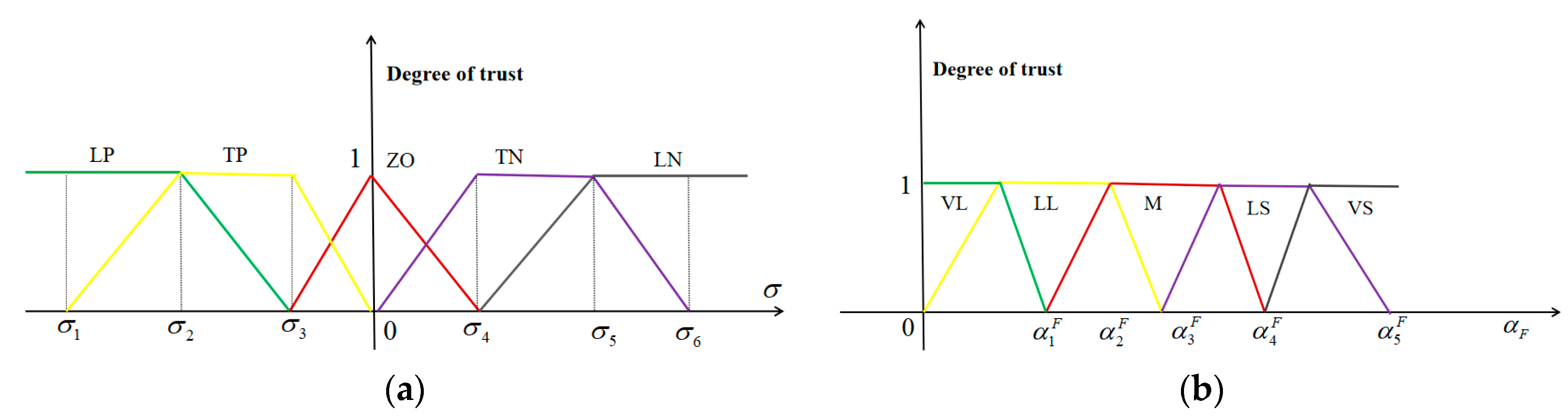
3.2. A Reinforcement Learning Method using a Fuzzy System

In order to reduce the learning cost, a learning method using a dynamic learning rate is a good solution [29]. For the reward function in the RL system, when the reward is positive after using the RL method, the influence of the positive feedback and a faster learning rate can be ensured by a high learning rate; on the contrary, a low learning rate can guide the RL method to a faster convergence. Therefore, there will be a relationship between the obtained reward and the value of the learning rate. Meanwhile, the reward is a fuzzy concept. For instance, a fixed value does not divide the “large positive number” and “large negative number”. So, a fuzzy system is used to develop a dynamic learning rate to improve the performance of this learning system. The reward r is taken as the input of the fuzzy system and the learning rate α F is taken as the output. We set the fuzzy description of r as “little negative number, the large negative number, zero, large positive number, little positive number”, and their abbreviations are shown as “TN, LN, ZO, LP, TP”. We set the fuzzy description of α F as “little small, very small, medium, very large, little large”, and their abbreviations are shown as “LS, VS, M, VL, LL”. Figure 2 gives the corresponding fuzzy membership functions. Previous work has shown that the performance of the fuzzy system is affected by the shape of the membership functions [30]. In the fuzzy system, triangular membership function and trapezoidal membership function are simple and effective, so we choose these two membership functions.
In Figure 2, { r i | i = 1 , 2 , , 6 } and { α i F | i = 1 , 2 , , 5 } are the division points that correspond to the input and output membership functions respectively. Five different input descriptions, “LP, TP, ZO, TN, LN” are { μ i r ( r ) | i = 1 , , 5 } , which correspond to each of these membership functions. Similarly, five fuzzy output descriptions, “VL, LL, M, LS, VS”, correspond to the output membership functions, expressed as { μ i α F ( α ) | i = 1 , , 5 } . Figure 2 shows the curve for these membership functions. The degree of trust for the input shows a general mathematical symmetry. We take “LP” as an example, and its membership function is shown in Equation (11).
μ 1 r ( r ) = { 1 , r < r 2 ( r 3 r ) / ( r 3 r 2 ) , r 2 < r < r 3 0 , r 3 < r
The number of discrete points for the input domain is represented by N r . We select five independent discrete points from the input domain, which are represented by I r = { I j r | j = 1 , , N r } . These five points have their own degrees of truth corresponding to five fuzzy input descriptions. Equation (12) gives the input degree for the truth discrete matrix I D r = [ I D i j r ] 5 × N r .
I D i j r = μ i r ( I j r )
The number of discrete points for the output domain is M α F . We select five independent discrete points O α F = { O j α F | j = 1 , , M α F } from the output domain. Equation (13) shows the corresponding output degree for the truth discrete matrix O D α F = [ O D i j α F ] 5 × M α F .
O D i j α F = μ i α F ( O j α F )
Then, we design the fuzzy rules, as follows. “If reward is “LP” then the learning rate is “VL”, If reward is “TP” then learning rate is “LL”, if reward if “ZO” then learning rate is “M”, if reward is “TN” then learning rate is “LS”, if reward is “LN” then learning rate is “VS””. The fuzzy inference is represented by R S r α F = [ r i j r α F ] N r × M α F and Equation (14) gives its mathematical expression.
r i j r α F = k = 1 5 ( I D k i r O D k j r )
where “ ” represents the operation of choosing the maximum value. “ ” represents the operation of choosing the minimum value. The operation of fuzzification transforms the reward r 0 into a fuzzy input vector F I r 0 = [ F I j r 0 ] 1 × N r if r 0 is measured. The degrees of the truth for r 0 corresponding to the five inputs are { μ i r 0 | μ i r 0 = μ i r ( r 0 ) ; i = 1 , , 5 } . Equation (15) uses the weighted-average method to calculate F I r 0 .
F I j r 0 = { i = 1 5 ( I D i j r × μ i r 0 ) } / k = 1 5 μ i r 0
We use the “min-max compose” operation to calculate the fuzzy output vector F O r 0 = [ F O j r 0 ] 1 × M α F using Equations (14) and (15).
F O j α F S = k = 1 N r ( r s k j F I k )
The de-fuzzifying operation uses a weighted average method to transform the fuzzy output into an output value and the weighted average method is shown in Equation (17).
α F S = { j = 1 M α F ( F O j α F S × O j α ) } / k = 1 M α F F O j α F S
where the learning rate α F S is the final result of the fuzzy system relative to r 0 .

4. A Proposed Learning Model for Multi-Robot Confrontation

The classical Q-learning algorithm chooses actions by the look-up table method. However, with the increase in action space and state space, the look-up table method is obviously no longer suitable, and which results in low learning efficiency. In order to solve this problem, the RL method based on the neural network approximating the value function of Q learning is proposed [31]. In the random task scenarios, the state variable s t is used as the input of the neural network and the Q value is used as the output of the neural network, which is also the estimation of the Q value of the neural network based on previous experience. This Q value is Q c u r r e n t , and the action that was taken by the agent is the action corresponding to the maximum Q c u r r e n t . After the agent takes action, the environment will give agent reward, and the state of the agent will be transferred to s t + 1 . Similarly, the state s t + 1 is input into the neural network, and the Q value of the corresponding state s t + 1 is obtained, which is Q n e x t . Finally, Q n e x t and Q c u r r e n t is used to update the Q value using (4). The gradient descent method is used to update the gradient of the neural network. The loss function L t of the neural network is shown in Equation (18).
L t = ( Q _ c u r r e n t * Q _ c u r r e n t ) = { ( 1 α ) Q _ c u r r e n t + α [ r t + γ max Q _ n e x t ] Q _ c u r r e n t }
where Q _ c u r r e n t * is the Q value after the state s t is updated by (4), and Q _ n e x t is the Q value before the state s t is updated.

4.1. Neural Network Model with Adaptive Momentum

Since the efficient action selection strategy should be considered for micromanagement scenarios, and our agent’s experience usually has a limited subset of the large state space, it will be difficult to apply the conventional reinforcement learning to learn an optimal policy. To address this problem, a BP neural network is used to approximate the state-action values to improve the generalization of our RL model. An acceleration algorithm using adaptive momentum is considered to be used in the BP neural network to ensure the efficiency of action selection.
In addition to the output layer and the input layer, the input signal of any neuron j in a layer is represented by n e t j . y j is the output signal. y j represents the output signal for the neuron i in the lower layer. Equation (19) gives the computing method for this output.
{ n e t j = i y i ω j i f ( x ) = ( 1 e b x ) a 1 + e b x y j = f ( θ j + i y i ω j i   )
where the constant a = 1.725, b = 0.566, the threshold for a neuron k is represented by θ k . In the output layer, y k is the label output signal for the k - th neuron. n e t k is the input signal. y k and n e t k are computed by Equation (20), if y j is the output signal of the neuron j - th in the hidden layer next to the output layer.
{ n e t k = j y j ω k j y k = f ( j y j ω k j + θ k )
In the t - th iteration for updating weight, an input value is x p ( t ) . O p k ( t ) , is the label output signal for the k - th neuron. y p k ( t ) is the actual output signal. Equation (21) gives the mean square error.
E p ( t ) = k ( O p k ( t ) y p k ( t ) ) 2 2
The weight of this neural network is updated by the back-propagation method. The mean square error of this neural network is given by Equation (22) if there are M n input values.
E p ( t ) = p k ( O p k ( t ) y p k ( t ) ) 2 2 M n
The weights ω k j ( t ) is updated according to the gradient direction of E p ( t ) to minimize the square error. The correction of ω k j ( t ) is Δ p ω k j ( t ) , which is given by:
{ E p ( t ) ω k j ( t ) = ( E p ( t ) n e t k ( t ) ) ( n e t u ( t ) ω k j ( t ) ) n e t u ( t ) ω k j ( t ) = j y p j ( t ) ω k j ( t )   ω k j ( t ) Δ p ω k j ( t ) = β Δ p ω k j ( t ) λ E p ( t ) ω k j ( t + 1 )
where the learning rate is λ and the momentum constant is β that is 0.95.
If the learning rate of the neural network is too large, the weight correction Δ p ω k j ( t ) will be too large, so the stability of the learning process will be affected. Therefore, we use an adaptive learning rate. α ( p ) represents the adaptive learning rate, and mean square error is E p ( t ) . The adaptive learning rate satisfies Equation (24).
α ( p ) = 1 exp ( E p ( t ) )
If the mean square error increases, the learning rate increases, and the convergence rate of the neural network accelerate; on the contrary, the neural network tends to be stable.
We set δ p k ( t ) = E p ( t ) n e t k ( t ) , and (25) can be obtained.
{ f ( θ k ( t ) + n e t k ( t ) ) = n e t k ( t ) ( 2 a 1 + exp ( F ( θ k ( t ) + n e t k ( t ) ) ) )   = ( 1 y p k ( t ) ) y p k ( t ) δ p k ( t ) = ( E p ( t ) n e t k ( t ) ) ( y p k ( t ) n e t k ( t ) )   = f ( θ k ( t ) + n e t k ( t ) ) ( O p k ( t ) y p k ( t )   )
Therefore, Equation (26) can be obtained.
{ Δ p ω k j ( t ) = β Δ p ω k j ( t ) δ p k ( t ) y p k ( t ) δ p k ( t ) = ( O p k ( t ) y p k ( t ) ) n e t k ( t ) ( 2 a 1 + exp ( F ( θ k ( t ) + n e t k ( t ) ) ) )  
The updating for the weights is given by Equation (27).
{ δ p j = E p n e t j = ( E p y p j ) ( y p j n e t j ) = y p j ( y p j 1 ) ( E p y p j ) Δ p ω j i = λ ( E p n e t j ) ( n e t j ω j i ) = λ y p j δ p j
where,
E p y p j = k ω k j δ p k = k ( E p n e t k ) ( n e t k y p j ) = k ( m y p m ω k m y p j ) y p j ( 1 y p j ) ( E p y p j )
Then,
δ p j = y p j ( y p j 1 ) ( δ p k ω k j )
Finally, Δ p ω j i = λ y p i δ p j is the correction of the weights for the hidden layer.

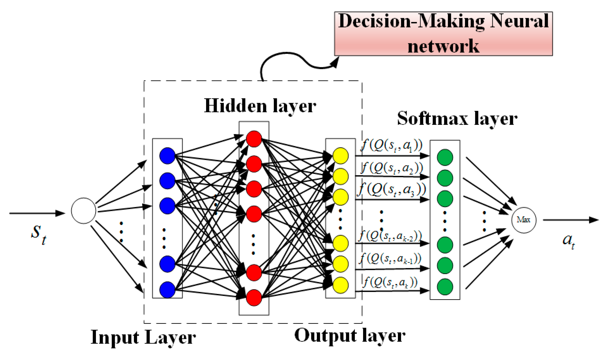
4.2. Multi-Agent RL Algorithm Based on Decision-Making Neural Network with Parameter Sharing

In this paper, an accelerated BP neural network with adaptive momentum is used as an approximator of the state-action value function. In this study, we extend the SSAQ algorithm to multi-agent by sharing the parameters of the neural network. Agents behave differently because each one receives different states and actions in the environment. Therefore, it is feasible for multi-agent to use the same neural network via parameter sharing. The input of the neural network is the agent state set in this paper, and the output is the state-action value function of the corresponding state. In order to ensure the continuous actions of the agent, a softmax layer is added after the output layer of the neural network, and the softmax layer uses the softmax function to select the action for the agent. Meanwhile, the simulated annealing algorithm is added to the softmax function to adjust the temperature parameters. This kind of neural network is called a decision-making neural network (DMNN) in this paper. The neural network is used as the approximator for the SSAQ algorithm mentioned above, and the learning model for our agents is shown in Figure 3.
As shown in Figure 4, the decision-making neural network includes an input layer, a multilayer hidden layer, an output layer, and a softmax layer. The state s t of the agent is inputted to the input layer of the decision-making neural network, and the Q value corresponding to the state s t is outputted to the output layer of the decision-making neural network, which is recorded as
{ Q ( s t , a t ; θ ) | i = 1 , 2 , , K t } .
where θ is the weight vector of the decision-making neural network. The Q values of all actions are entered into the softmax layer with a non-linear transformation function which is shown in Equation (30), and the action a t is selected and outputted using the Max operation as shown in Equation (31).
ϕ ( x ) = exp ( x ) / T i
max { ϕ ( x 1 ) / i = 1 m ϕ ( x i ) , ϕ ( x 2 ) / i = 1 m ϕ ( x i ) , , ϕ ( x m ) / i = 1 m ϕ ( x i ) }
The agent takes action a t and the environment gives instant rewards R ( t ) . The RL based on state-action function stores the state-action function in the form of a table, but this method cannot solve the large-scale continuous state-space problem, and the powerful generalization ability of the neural network is used to approximate the value function Q ( s t , a t ; θ ) for RL, which solves the problem of high dimensional continuous state space. The proposed method has a good generalization and can be used in other combat games, such as Starcraft II [18].
To update the weights of the neural network efficiently, the TD error of the RL method is used for the Loss function for the decision-making neural network. The TD error is shown in Equation (32). The back propagation algorithm is used to update the weights of neural networks. The Multi-agent SSAQ algorithm with network parameter sharing is given by Algorithm 2.
{ Q n e x t ( s t , a t , θ t ) = Q ( s t , a t , θ t ) c u r + α [ R ( t ) + γ Q ( s t + 1 , a t + 1 , θ t ) Q ( s t , a t , θ t ) c u r ] ϕ t = Q n e x t ( s t , a t , θ t ) Q ( s t , a t , θ t ) c u r
Algorithm 2: Multi-agent SSAQ algorithm
Definition
T t : = Current temperature parameters
T t + 1 : = Next temperature parameters
T min : = Minimum temperature parameter
T max : = Maximum temperature parameter
α t : = Adaptive learning rate of the neural network
γ : = Discount factor
K t : = The number of actions in t time
f u n ( ) : = Updating state-action function in SMDP
Initialization
 Initialize s t , a t , s t + 1 , a t + 1 , r t
Repeat (for each step)
 Choose an initial state s 0
t 0 ; i 0 ;
Repeat (for each step of the episode)
P ( a t | s t ) = max p s : 1 K t P ( a k p s | s t ) = max p s : 1 K t exp [ Q ( s t , a k p s ) / T t ] k = 1 K t exp [ Q ( s t , a k ) / T t ] a t
 Observe s t + 1 , after T learning cycles by the same actions a t
 Obtain reward r t , r t + 1 , , r t + T 1
P ( a t + 1 | s t + 1 ) = max p s : 1 K t P ( a k p s | s t + 1 ) = max p s : 1 K t exp [ Q ( s t + 1 , a k p s ) / T t ] k = 1 K t exp [ Q ( s t + 1 , a k ) / T t ] a t + 1
 Update TD error and weights:
ϕ t α [ f ( Q ( s t + 1 , a t + 1 ) , r t , , r t + T 1 , α , γ ) Q ( s t , a t , θ t ) ]
E t 1 2 ϕ t 2 ; α t 1 exp ( E t )
θ t + 1 θ t + α t ϕ t
t + +
until s is terminal.

5. Curriculum Transfer Learning

Curriculum Transfer Learning for Different Micromanagement Scenarios

It will cost a lot of time if the agent starts learning from scratch in a new environment. Many researchers focus on improving the learning performance by exploiting domain knowledge between some related tasks. The prior learning experience is exploited from the source task to the target task by the transfer learning to accelerate the learning rate. Therefore, we use the transfer learning method to take the well-trained model of source task as the prior experience to build the learning model to the target task.
In the curriculum transfer learning for micromanagement scenarios in the confrontation decision-making system, the mapping ρ : π p a s t t i m e * π c u r r e n t t i m e * represents the process that transfers the learning policy of the source task to the learning policy of the target task. In this paper, the state space and action space remain unchanged, as shown in Equation (33).
{ ρ A : A l a s t   t i m e A c u r r e n t   t i m e ρ S : S l a s t   t i m e S c u r r e n t   t i m e
Many interference information exists in the learning process. Therefore, we set up a decay function using the Newton law of cooling. The decay function enables agents to exploit the domain knowledge with a decreasing probability. A steady-state is achieved eventually. The threshold is ε . Equation (34) shows the mathematical relationship between the threshold ε and time t . The agent uses the domain knowledge from the source task if the random number ε < r a n d o m . Otherwise, the agent uses the conventional maximum Q value strategy to select an action.
ε ( t ) = ε ( t 0 ) exp { p t + p t 0 }
where the decay coefficient is p and the initial time is t 0 . The probability of using the prior experience from the source task gradually decreases until a stable value is achieved.
If the target task is too difficult compared with the source task, an intermediate task is usually set up in curriculum transfer learning, and the agent can gain more experience by the learning model for the intermediate task. The curriculum transfer learning with an intermediate task and decay function for micromanagement scenarios is shown in Figure 5.
The integral framework for the proposed learning model for micromanagement is shown in Figure 6. The proposed method has three parts: the decision-making neural network, the loss function that uses the TD error for the neural network and a fuzzy method. The state s t of the agent is input into the neural network, and the neural network outputs the action a t . So is the next state s t + 1 . The reward R ( t ) is obtained. The TD error is calculated as a loss function and a fuzzy method is used to adjust the learning rate of the RL method.

6. Experiment and Analysis

Generally, in the robotic systems that are based on reinforcement learning, higher learning rates enable robots to utilize the previous learning experience. The larger discount rate makes learning agents think more about long-term returns in the future. For the exploration and exploitation, the ε-greedy algorithm with a larger threshold allows the learning agent to more utilize prior experience. In this work, the initial value for the threshold of the decay function is the same as that of the classical ε-greedy algorithm. In these experiments, the values for the learning rate, the discount factor, the Exploring rate, the Annealing factor, the Maximum temperature parameter, and the Minimum temperature parameter are given manually and empirically.

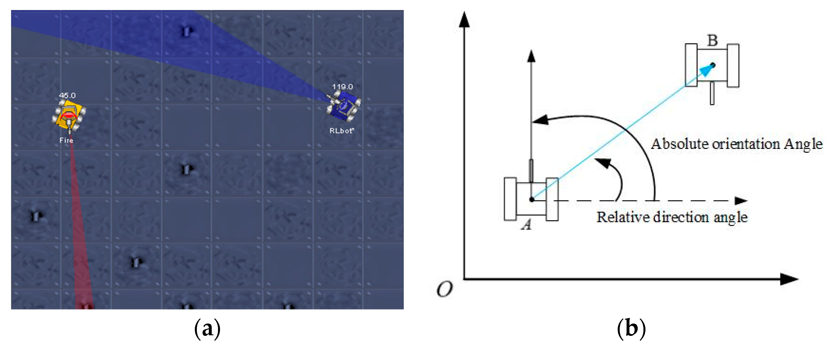
6.1. RL Model for a Confrontation Decision-Making System

Robocode [32,33] is an open-source platform, where the goal is to develop a robot to battle against other robots. The platform is shown in Figure 7. In this paper, the experiments are conducted in this platform and we consider several scenarios with the different enemies to test the generalization of the proposed method.
Effective state-action space definition of the RL model is still an open problem with no universal solution. An RL model for robot confrontation with inputs from the game engine is constructed, which ensures the size of the state-action space remaining unchanged to avoid the curse of dimensionality.
State-space: The combination of the relative direction angle, the absolute orientation angle, and the distance between the robots form the state space. The absolute direction angle and the relative direction angle are discretized into four kinds of states and the range of absolute direction angle is 0 ~ 360 . We divide the distance between the robots into 20 discrete parts.
Action space: Movement and rotation are two movements for the robot in this platform. At each time step, each robot can move to arbitrary directions with arbitrary distances in the ground. Similar to other types of combat games, our robot can choose to attack their opponents with bullets of different energies. Forward, backward, clockwise rotation and anticlockwise rotation four kinds of different movements form the action space.
Reward function: If a robot fires bullets hit the enemy or is hit by bullets, the health point of this robot will change. We propose a reward function to help agent balance losses of our and opponents, as shown in:
r e w a r d ( t ) = ( ( E t m E t 1 m ) ( E t e E t 1 e ) ) | E t 1 e E t e | | E t m E t 1 m |
In this reward function, E t m represents the health point of our agent at t time, E t 1 m represents the health point of our agent at the t−1 time, E t e represents the health point of the opponent at the t time and E t 1 e represents the health point of the opponent at the t−1 time. If we lose fewer health points than the opponent loses, we will get a positive reward. The ratio of absolute health point changes between the two sides will encourage our agent to hurt the opponent more in battle. According to the experimental results, the RL model is effective at controlling our agent in the micromanagement scenarios.

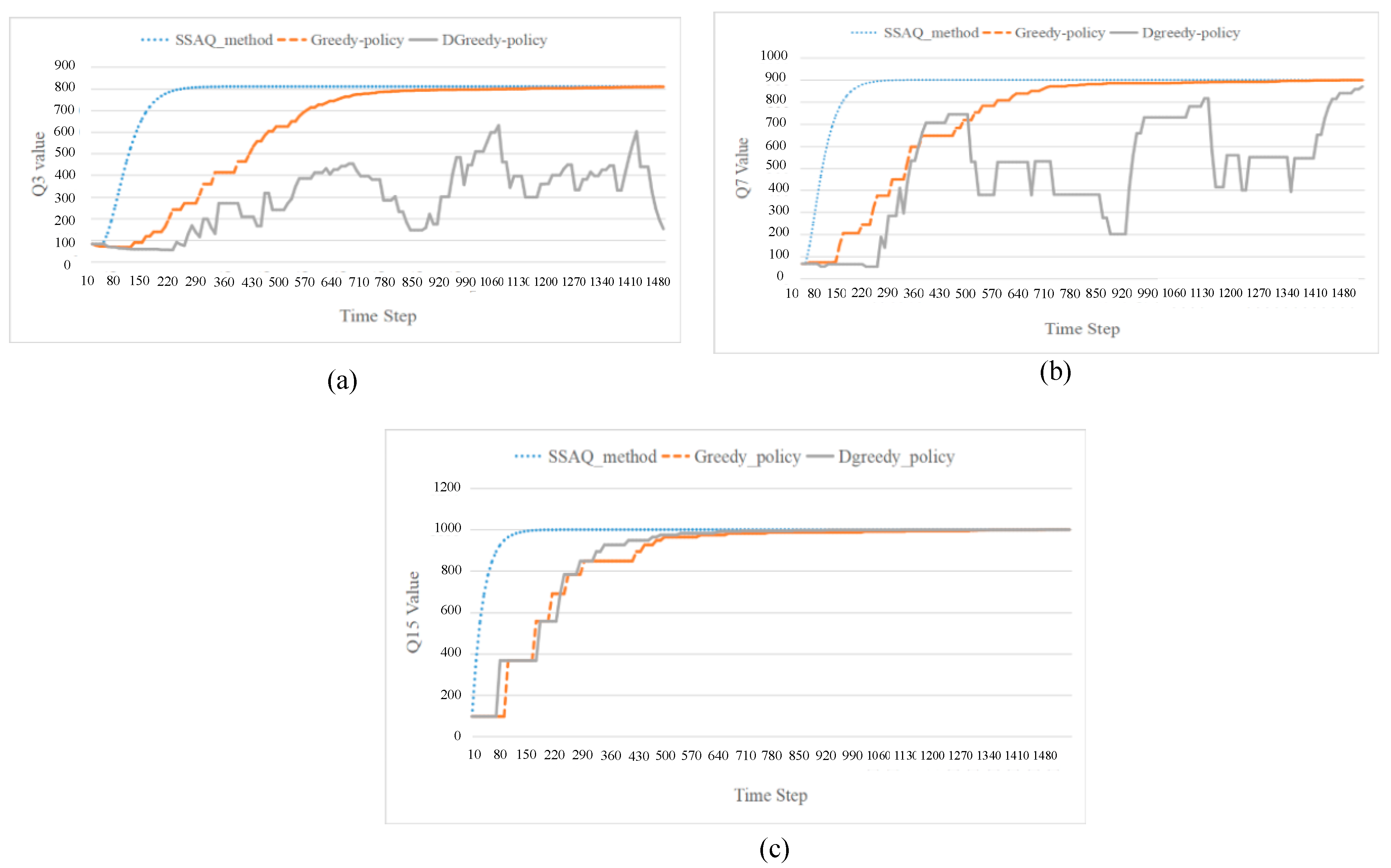
6.2. Proposed RL Algorithm Test

In order to verify the effectiveness of the proposed SSAQ algorithm, a comparative experiment of robot migration is designed. The map for robot migration satisfies the binary tree structure. As shown in Figure 8, there are N layers on the map, and the number of endpoints is 2 N 1 .
The robot can get the reward corresponding to each endpoint by starting from the beginning and repeating the branch to the bottom endpoint. A total of 2 N 1 actions can be selected by the robot. The corresponding Q values of each endpoint are expressed as Q 1 ~ Q 2 N 1 . When the robot reaches the endpoint 2 N 1 , it gets a reward of +1000, and it does not get a reward reaching the rest of the endpoints. Q values can be obtained through experiments. This paper uses the SSAQ method to compare with the ε-greedy policy (Greedy-policy) and ε-greedy policy using the decay threshold (Dgreedy-policy) [34]. The settings of parameters for this experiment are listed in Table 1.
Through the observation during the experiments, it shows that Q 3 , Q 7 and Q 15 will change in the experiment, and we record these Q values. Therefore, the changes in three kinds of Q values of Q 3 , Q 7 and Q 15 are used in the experiment to compare three different strategies. As shown in Figure 9, the convergence time of the proposed method (SSAQ algorithm) is 214, 168 and 122 for Q 3 , Q 7 and Q 15 , respectively. The convergence time of the proposed method is the shortest and the convergence rate of it is the fastest compared with the other two methods. In addition, the Q-value curve of the proposed strategy is relatively smooth, which also proves that the proposed strategy is more stable and can achieve the target state quickly while ensuring the stability of learning performance.

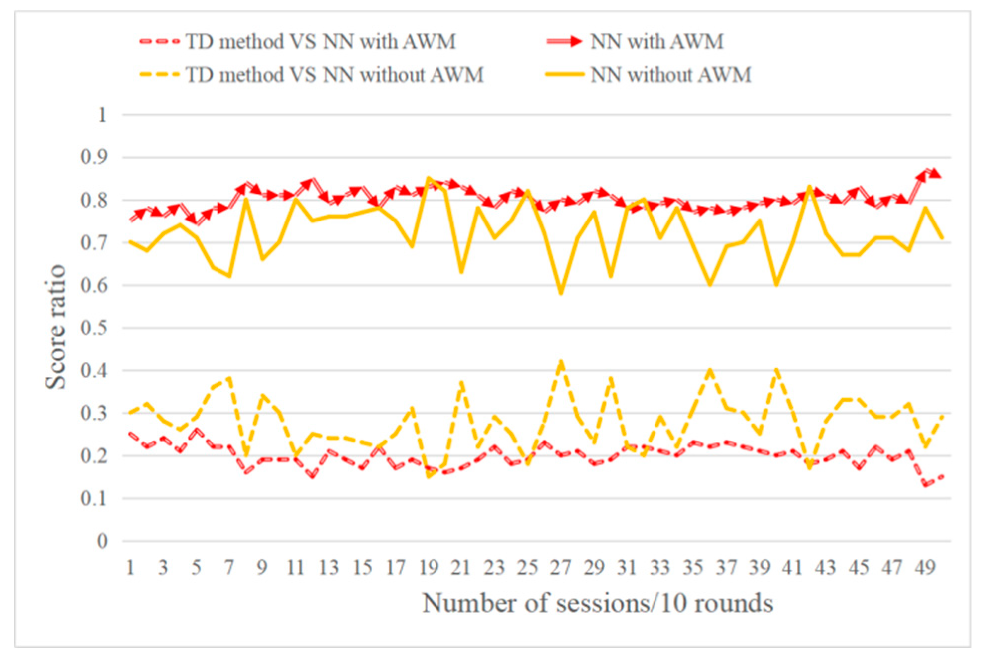
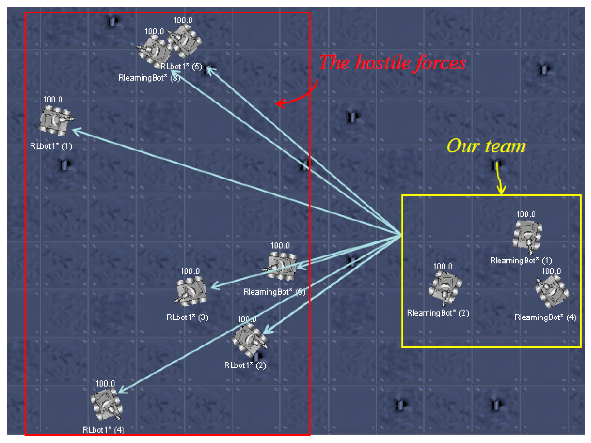
6.3. Effect Test for Multi-Agent RL Based on DMNN and Fuzzy Method

The convergence and stability of the neural network are important factors affecting the performance of micromanagement for an agent. Hence, this paper proposes a decision-making neural network with adaptive momentum. In order to verify the effectiveness of the proposed Multi-agent RL algorithm based on DMNN, a team of agents trained by the neural network with adaptive momentum (NN with AWM) and another team of tank agents trained by the neural network without adaptive momentum (NN without AWM) are used to fight the team of tank agents trained by TD method separately. Each team has four tank agents. The settings of parameters for this experiment are listed in Table 2.
We compare “NN with AWM” and “NN without AWM” from three different perspectives: total score ratio, defensive score and fluctuation value of score ratio. The number of rounds is 500, and the score is recorded every 10 rounds. Every 10 rounds are called a session. Figure 10, Figure 11 and Figure 12 represent the resulting curve of this experiment, in which the horizontal axis represents the number of sessions and the vertical axis represents the score ratio or fluctuation value or defensive score. This paper calculates the first-order difference of the total score ratio, that is, S c o r e   r a t i o t + 1 S c o r e   r a t i o t , and obtains the fluctuation value curve of the total score ratio, as shown in Figure 11. From the experimental results, it can be seen that these score ratios of the tank agents trained by the NN with the AWM method are obviously higher than the NN without AWM method, and the fluctuation value is relatively small. Figure 12 shows the curve of the defensive score. Similar to Figure 10, the defensive score of the NN with the AWM method is more stable and higher than the NN without the AWM method. The experimental results show that the proposed Multi-agent RL algorithm can not only make the tank agent get higher scores in combat, but also get more stable scores. Hence, we can see that the proposed method has outstanding performances for micromanagement.
A fuzzy method is used to tuning the learning rate for the RL model. The input domain of the fuzzy method is set as { r i | i = 1 , 2 , , 7 } = { 30 , 20 , 10 , 0 , 10 , 20 , 30 } , and the output domain of the fuzzy method is set as { α i | i = 1 , 2 , , 7 } = { 0.95 , 0.80 , 0.65 , 0.50 , 0.35 , 0.20 , 0.05 } . The number of discrete points is 7. According to the fuzzy method used in this paper, the results of the fuzzy system are shown in Figure 13. As shown in Figure 13, the fuzzy method converts the linear input into the smooth output, which is appropriate for micromanagement in the Multi-Robot Confrontation system. Then, the experimental results of the fuzzy-inspired learning model (FLM), learning model (LM) with learning rate being 0.2 (LM-0.2) [12] and learning model with learning rate being 0.95 (LM-0.95) are tested in the Robocode platform, as shown in Figure 14.
The three methods of FLM, LM-0.2, and LM-0.95 were respectively fought with the TD method. The solid line represents the score of three methods respectively, while the dotted lines represent the scores of TD methods fighting against three methods. From Figure 14, in FLM, the score ratio remains at around 0.8. In LM-0.2 and LM-0.95, the score ratio remains at around 0.7. According to the above results, it can be obtained that the fuzzy method can get a higher score in combat than the method of the fixed learning rate for micromanagement.

6.4. Effect Test for Curriculum Transfer Learning (TF)

Six tank agents trained by the TD method are formed, which is called “TD_team”, and the multiple robots in formation will not attack each other. Then, the learning model proposed in this paper is used to fight the TD_team. Compared to the above experiments, our tank agents will face six opponents at the same time, as shown in Figure 15. In Figure 15, The agent in the red box is the enemy team, while the agent in the yellow box is our team.
In order to prove the efficiency and practicality of the learning model with curriculum transfer learning (LM with TF), it is compared with the learning model without curriculum transfer learning (LM without TF) for 500 rounds.
The tank agent using curriculum transfer learning will use the prior experience gained in the above experiments. From Figure 16, transfer learning accelerates the learning speed of tank agents in the new micromanagement scenario and achieves higher scores than the method without transfer learning. From Figure 17, it is obvious that the defensive score of the LM with the TF method is higher, which means that the agent can defend the opponent’s attack well when attacking opponents. Ten tank agents trained by the TD method were formed, and then the LM with the TF method and the LM without TF method were used to fight against them respectively. The task of fighting TD_team is regarded as the intermediate task of this task because it is more difficult than the original task. From Figure 18, the score ratio of the LM with the TF method is still higher than that of the LM without the TF method, which means the learning model with curriculum transfer learning has a strong and stable property for micromanagement scenarios in confrontation decision-making system.

7. Conclusions

In this paper, the confrontation decision-making for micromanagement scenarios in SMDP is studied. This paper makes several contributions, including an improved Q-learning in SMDP (SSAQ algorithm) for confrontation decision-making, the fuzzy method for adjusting learning rate of the RL method, Multi-agent RL algorithm with parameter sharing, accelerated neural network for the representation of state (DMNN) and a curriculum transfer learning method with decay function. The RL model designed ensures the size of the state-action space remaining unchanged to avoid the curse of dimensionality and the reward function to help agent balance losses of our agents and opponents. The decision-making neural network uses adaptive momentum, which is used as an approximator to estimate the state-action function. The accelerated algorithm using adaptive momentum allows the decision-making neural network to react quickly in micromanagement scenarios. Finally, the curriculum transfer learning method with the decay function extends our model to other different scenarios. The proposed transfer learning method can still achieve better experimental results in more complex confrontation scenarios. The results of experiments demonstrate proposed methods can achieve an excellent and stable control for micromanagement in robot confrontation system. In the future, we will extend this model to the game scenario of Starcraft II. In addition, the behavior decomposition methods [35,36,37,38] will be studied to achieve more advanced Multi-agent confrontation strategies.

Author Contributions

C.H. and M.X. conceived the idea of the paper. C.H. and M.X. designed and performed the experiments; C.H. and M.X. analyzed the data; C.H. contributed reagents/materials/analysis tools; C.H. wrote and revised the paper.

Funding

This work is supported in part by the Natural Science Foundation of Hubei Province under Grant 2013CFC026, the Shaanxi Province Key Research and Development Program of China under Grant 2018GY-187.

Conflicts of Interest

The authors declare no conflict of interest.

References

  1. Weron, R. Electricity price forecasting: A review of the state-of-the-art with a look into the future. Int. J. Forecast. 2014, 4, 1030–1081. [Google Scholar] [CrossRef]
  2. Ferreira, L.N.; Toledo, C.; Tanager, A. Generator of Feasible and Engaging Levels for Angry Birds. IEEE Trans. Games 2017, 10, 304–316. [Google Scholar] [CrossRef]
  3. Hiller, J.; Reindl, L.M. A computer simulation platform for the estimation of measurement uncertainties in dimensional X-ray computed tomography. Measurement 2012, 45, 2166–2182. [Google Scholar] [CrossRef]
  4. Mnih, V.; Kavukcuoglu, K.; Silver, D.; Rusu, A.A.; Veness, J.; Bellemare, M.G.; Graves, A.; Riedmiller, M.; Fidjeland, A.K.; Ostrovski, G. Human-level control through deep reinforcement learning. Nature 2015, 518, 529–533. [Google Scholar] [CrossRef] [PubMed]
  5. Moravik, M.; Schmid, M.; Burch, N.; Lisy, V.; Morrill, D.; Bard, N.; Davis, T.; Waugh, K.; Johanson, M.; Bowling, M. Deepstack: Expert level artificial intelligence in heads-up no-limit poker. Science 2017, 356, 508–513. [Google Scholar] [CrossRef]
  6. Yao, W.; Lu, H.; Zeng, Z.; Xiao, J.; Zheng, Z. Distributed Static and Dynamic Circumnavigation Control with Arbitrary Spacings for a Heterogeneous Multi-robot System. J. Intell. Robot. Syst. 2018, 4, 1–23. [Google Scholar] [CrossRef]
  7. Ontanon, S.; Synnaeve, G.; Uriarte, A.; Richoux, F.; Churchill, D.; Preuss, M.A. Survey of Real-Time Strategy Game AI Research and Competition in StarCraft. IEEE Trans. Comput. Intell. AI Games 2013, 5, 293–311. [Google Scholar] [CrossRef]
  8. Synnaeve, G.; Bessiere, P. Multiscale Bayesian Modeling for RTS Games: An Application to StarCraft AI. IEEE Trans. Comput. Intell. AI Games 2016, 8, 338–350. [Google Scholar] [CrossRef]
  9. Thrun, S.; Littman, M.L. Reinforcement Learning: An Introduction. IEEE Trans. Neural Netw. 2005, 16, 285–286. [Google Scholar]
  10. Shi, H.; Li, X.; Hwang, K.S.; Pan, W.; Xu, G. Decoupled Visual Servoing With Fuzzy Q-Learning. IEEE Trans. Ind. Inform. 2018, 14, 241–252. [Google Scholar] [CrossRef]
  11. Shi, H.; Lin, Z.; Zhang, S.; Li, X.; Hwang, K.S. An adaptive Decision-making Method with Fuzzy Bayesian Reinforcement Learning for Robot Soccer. Inform. Sci. 2018, 436, 268–281. [Google Scholar] [CrossRef]
  12. Xu, M.; Shi, H.; Wang, Y. Play games using Reinforcement Learning and Artificial Neural Networks with Experience Replay. In Proceedings of the 2018 IEEE/ACIS 17th International Conference on Computer and Information Science (ICIS), Singapore, 6–8 June 2018; pp. 855–859. [Google Scholar]
  13. Cincotti, S.; Gallo, G.; Ponta, L.; Raberto, M. Modeling and forecasting of electricity spot-prices: Computational intelligence vs. classical econometrics. AI Commun. 2014, 3, 301–314. [Google Scholar]
  14. Geramifard, A.; Dann, C.; Klein, R.H.; Dabney, W.; How, J.P. RLPy. A value-function-based reinforcement learning framework for education and research. J. Mach. Learn. Res. 2015, 16, 1573–1578. [Google Scholar]
  15. Modares, H.; Lewis, F.L.; Jiang, Z.P. Optimal Output-Feedback Control of Unknown Continuous-Time Linear Systems Using Off-policy Reinforcement Learning. IEEE Trans. Cybern. 2016, 46, 2401–2410. [Google Scholar] [CrossRef] [PubMed]
  16. Konda, V. Actor-critic algorithms. Siam J. Control Optim. 2003, 42, 1143–1166. [Google Scholar] [CrossRef]
  17. Patel, P.G.; Carver, N.; Rahimi, S. Tuning computer gaming agents using Q-learning. In Proceedings of the Computer Science and Information Systems (FedCSIS), Szczecin, Poland, 18–21 September 2011; pp. 581–588. [Google Scholar]
  18. Shao, K.; Zhu, Y.; Zhao, D. StarCraft Micromanagement with Reinforcement Learning and Curriculum Transfer Learning. IEEE Trans. Emerg. Top. Comput. Intell. 2018, 3, 73–84. [Google Scholar] [CrossRef]
  19. Xu, D.; Shao, H.; Zhang, H.A. New adaptive momentum algorithm for split-complex recurrent neural networks. Neurocomputing 2012, 93, 133–136. [Google Scholar] [CrossRef]
  20. Lecun, Y.; Bengio, Y.; Hinton, G. Deep learning. Nature 2015, 521, 436. [Google Scholar] [CrossRef]
  21. Peng, P.; Yuan, Q.; Wen, Y.; Yang, Y.; Tang, Z.; Long, H.; Wang, J. Multi-agent bidirectionally-coordinated nets for learning to play StarCraft combat games. arXiv 2017, arXiv:1703.10069. [Google Scholar]
  22. Pan, S.J.; Yang, Q. A Survey on Transfer Learning. IEEE Trans. Knowl. Data Eng. 2010, 22, 1345–1359. [Google Scholar] [CrossRef]
  23. Gil, P.; Rez, M.; Mez, M.; Gómez, A.F.S. Building a reputation-based bootstrapping mechanism for newcomers in collaborative alert systems. J. Comput. Syst. Sci. 2014, 80, 571–590. [Google Scholar]
  24. Bertsimas, D.; Tsitsiklis, J. Simulated Annealing. Stat. Sci. 1993, 8, 10–15. [Google Scholar] [CrossRef]
  25. Shi, H.; Yang, S.; Hwang, K.; Chen, J.; Hu, M.; Zhang, H. A Sample Aggregation Approach to Experiences Replay of Dyna-Q Learning. IEEE Access 2018, 6, 37173–37184. [Google Scholar] [CrossRef]
  26. Shi, H.; Xu, M.; Hwang, K. A Fuzzy Adaptive Approach to Decoupled Visual Servoing for a Wheeled Mobile Robot. IEEE Trans. Fuzzy Syst. 2019. [Google Scholar] [CrossRef]
  27. Shi, H.; Lin, Z.; Hwang, K.S.; Yang, S.; Chen, J. An Adaptive Strategy Selection Method with Reinforcement Learning for Robotic Soccer Games. IEEE Access 2018, 6, 8376–8386. [Google Scholar] [CrossRef]
  28. Choi, S.Y.; Le, T.; Nguyen, Q.; Layek, M.A.; Lee, S.; Chung, T. Toward Self-Driving Bicycles Using State-of-the-Art Deep Reinforcement Learning Algorithms. Symmetry 2019, 11, 290. [Google Scholar] [CrossRef]
  29. Zhao, G.; Tatsumi, S.; Sun, R. RTP-Q: A Reinforcement Learning System with Time Constraints Exploration Planning for Accelerating the Learning Rate. IEICE Trans. Fundam. Electron. Commun. Comput. Sci. 1999, 82, 2266–2273. [Google Scholar]
  30. Basyigit, A.I.; Ulu, C.; Guzelkaya, M. A New Fuzzy Time Series Model Using Triangular and Trapezoidal Membership Functions. In Proceedings of the International Work-Conference On Time Series, Granada, Spain, 25–27 June 2014; pp. 25–27. [Google Scholar]
  31. Zhou, Q.; Shi, P.; Xu, S.; Li, H. Observer-based adaptive neural network control for nonlinear stochastic systems with time delay. IEEE Trans. Neural Netw. Learn. Syst. 2012, 24, 71–80. [Google Scholar] [CrossRef]
  32. Harper, R. Evolving Robocode tanks for Evo Robocode. Genet. Program. Evol. Mach. 2014, 15, 403–431. [Google Scholar] [CrossRef]
  33. Woolley, B.G.; Peterson, G.L. Unified Behavior Framework for Reactive Robot Control. J. Intell. Robot. Syst. 2009, 55, 155–176. [Google Scholar] [CrossRef]
  34. Auer, P.; Cesabianchi, N.; Fischer, P. Finite-time Analysis of the Multiarmed Bandit Problem. Mach. Learn. 2002, 47, 235–256. [Google Scholar] [CrossRef]
  35. Shi, H.; Xu, M. A Multiple Attribute Decision-Making Approach to Reinforcement Learning. IEEE Trans. Cogn. Dev. Syst. 2019. [Google Scholar] [CrossRef]
  36. Shi, H.; Xu, M. A Data Classification Method Using Genetic Algorithm and K-Means Algorithm with Optimizing Initial Cluster Center. In Proceedings of the 2018 IEEE International Conference on Computer and Communication Engineering Technology (CCET), Beijing, China, 18–20 August 2018; pp. 224–228. [Google Scholar]
  37. Xu, M.; Shi, H.; Jiang, K.; Wang, L.; Li, X.A. Fuzzy Approach to Visual Servoing with A Bagging Method for Wheeled Mobile Robot. In Proceedings of the 2019 IEEE International Conference on Mechatronics and Automation, Tianjin, China, 4–7 August 2019; pp. 444–449. [Google Scholar]
  38. Shi, H.; Xu, M.; Hwang, K.; Cai, B.Y. Behavior Fusion for Deep Reinforcement Learning. ISA Trans. 2019. [Google Scholar] [CrossRef] [PubMed]
Figure 1. Reinforcement learning architecture.
Information 10 00341 g001
Figure 2. Curves for the Membership functions. (a) Reward/Input membership function. (b) Learning rate/Output membership function.
Information 10 00341 g002
Figure 3. The learning model of agent architecture. The decision-making neural network is used as the approximator for the state-action function.
Information 10 00341 g003
Figure 4. Decision-making neural network architecture.
Information 10 00341 g004
Figure 5. Curriculum transfer learning with an intermediate task and decay function.
Information 10 00341 g005
Figure 6. Framework for the proposed method for micromanagement.
Information 10 00341 g006
Figure 7. Robot confrontation platform. (a) a platform for the tank battle system, (b) diagram of absolute and relative angles.
Information 10 00341 g007
Figure 8. The experiment for robot migration.
Information 10 00341 g008
Figure 9. The comparison curve of Q value: (a) The change curve of Q 3 ; (b) The change curve of Q 7 ; (c) The change curve of Q 15 .
Information 10 00341 g009
Figure 10. The comparison curve of the total score ratio.
Information 10 00341 g010
Figure 11. The curve of the fluctuation value of the total score ratio.
Information 10 00341 g011
Figure 12. The curve of the Defensive score. (a) The defensive score of neural network (NN) without adaptive momentum (AWM); (b) The defensive score of NN with AWM.
Information 10 00341 g012
Figure 13. Results of the fuzzy method.
Information 10 00341 g013
Figure 14. Comparison of learning results for different learning rates.
Information 10 00341 g014
Figure 15. Simulation experiments for the TF method.
Information 10 00341 g015
Figure 16. Comparisons of learning models in score ratio. One model uses transfer learning, the other does not use transfer learning.
Information 10 00341 g016
Figure 17. Comparisons of learning models in the defensive score. (a) The defensive score for LM with TF and TD_team; (b) Defensive score for LM without TF and TD_team.
Information 10 00341 g017
Figure 18. Comparisons of learning models in score ratio.
Information 10 00341 g018
Table 1. Experimental parameters.
ParameterValue
Learning rate α 0.3
Discount rate γ 0.9
Exploring rate ε 0.9
Annealing factor η 0.9
Maximum temperature parameter T max 0.1
Minimum temperature parameter T min 0.01
Layers of the map N 10
Table 2. Experimental parameters.
ParameterValue
Learning rate of RL α 0.1
Discount rate γ 0.9
Exploring rate ε 0.95
Annealing factor η 0.9
Maximum temperature parameter T max 0.1
Minimum temperature parameter T min 0.01
Learning rate of Neural network α 0.9
Momentum constant β 0.95

