Approximate Completed Trace Equivalence of ILAHSs Based on SAS Solving

Abstract

The ILAHS (inhomogeneous linear algebraic hybrid system) is a kind of classic hybrid system. For the purpose of optimizing the design of ILAHS, one important strategy is to introduce equivalence to reduce the states. Recent advances in the hybrid system indicate that approximate trace equivalence can further simplify the design of ILAHS. To address this issue, the paper first introduces the trajectory metric $d_{trj}$ for measuring the deviation of two hybrid systems’ behaviors. Given a deviation $\epsilon \ge 0$, the original ILAHS of ${\mathcal{H}}_1$ can be transformed to the approximate ILAHS of ${\mathcal{H}}_2$, then in trace equivalence semantics, ${\mathcal{H}}_2$ is further reduced to ${\mathcal{H}}_3$ with the same functions, and hence ${\mathcal{H}}_1$ is $\epsilon$-approximate trace equivalent to ${\mathcal{H}}_3$. In particular, $\epsilon =0$ is a traditional trace equivalence. We implement an approach based on RealRootClassification to determine the approximation between the ILAHSs. The paper also shows that the existing approaches are only special cases of our method. Finally, we illustrate the effectiveness and practicality of our method on an example.

1. Introduction

In the real world, there exist many systems exhibiting a hybrid discrete–continuous behavior, and the notion of hybrid automaton [1] was introduced to model these hybrid systems. For example, embedded systems are often modeled as hybrid systems due to their involvement of both digital control software and analog plants, which physical process is often specified in the form of differential equations. Infinite states (or state explosion) due to the continuous behavior of the system are among the most challenging problems in verifying hybrid systems. In the traditional functional analysis domain, an efficient classical technique to tackle state explosion is equivalence [2,3]. In brief, the systems with the same functional behaviors are called equivalence. Functional equivalence simplifies the system by removing the duplicate branches. The papers by Glabbeek [2,3] proposed fourteen kinds of linear time-branching time equivalence relations, and the completed trace equivalence is a basic state-space equivalence relation, which can be used to further reduce the states of hybrid systems [4,5].

However, traditional equivalence techniques are based on absolute precision, which only gives the answer “yes” or “no”, not how much simulation. There is an example that illustrates that it is meaningful to introduce the deviation analysis to equivalence. Considering a microwave oven, if the microwave oven is required to heat to 100 ${}^{\circ }$C within 60 s but does so within 60.5 s (this is very common in life), and if a 0.5 s deviation is allowable, then the two systems are equivalent, or the two states can be merged. Otherwise, the two systems are not equivalent, or the two states cannot be merged. Especially in safety-critical cases, any deviation greater than zero seconds can be viewed as the presence of a bug. In reality, the parameters of hybrid systems are obtained by all kinds of measurements, which generally have a small number of errors. Since errors are inevitable, approximation analysis between the original system and the approximate system is very significant for the given permission precision.

In order to achieve this goal, this paper proceeds by defining two types of metrics, state metric $d_{sta}$ and trajectory metric $d_{trj}$, to check how much a hybrid system ${\mathcal{H}}_1$ conforms to another hybrid system ${\mathcal{H}}_2$. The $d_{sta}$ measures the distance of the states, while the $d_{trj}$ specifies the deviation of the system behaviors. Given a deviation $\epsilon \ge 0$, the original ILAHS of ${\mathcal{H}}_1$ can be transformed to the approximate ILAHS of ${\mathcal{H}}_2$. Then in trace equivalence semantics, ${\mathcal{H}}_2$ is further reduced to ${\mathcal{H}}_3$ with the same functions, and hence ${\mathcal{H}}_1$ is $\epsilon$-approximate trace equivalent to ${\mathcal{H}}_3$. In particular, $\epsilon =0$ is a traditional trace equivalence. At last, the decision problem that ${\mathcal{H}}_1$ is $\epsilon$-approximate to ${\mathcal{H}}_2$ can be reduced to semi-algebraic system solving (SAS solving) [6,7,8,9,10,11].

There are several choices for metrics, such as bisimulation metrics [12,13], Lyapunov-like functions [13], directed metrics [14], and pseudo-ultrametrics [15], most of which are required to satisfy intricate properties of simulation or bisimulation relations. In contrast, state metric $d_{sta}$ and trajectory metric $d_{trj}$ in this paper are based on Euclidean distance, which is an intuitive metric.

In this paper, we focus on a specific class of hybrid systems, namely, inhomogeneous linear algebraic hybrid systems (ILAHSs for short). It is well known that the most important analysis question for hybrid systems is the problem of reachability, which is computationally hard and undecidable for the general case and intractable even for the simplest subclasses [1]. So it is doomed to be impossible to find a universal approach for this question without any simplifications or restrictions. ILAHSs, which are ubiquitous in reality, are a kind of classical hybrid systems with some simplifications.

Note that our approximation technology differs from those proposed in the papers [16,17,18,19,20], which aim to construct an approximately reachable set. Most of the differential equations of hybrid systems, as we all know, cannot be solved analytically, and, therefore, the exact reachable set cannot be computed symbolically, so many papers developed a variety of methods that over-approximate or under-approximate the reachable set using varieties of set representations such as polyhedra [21], zonotopes [22], level sets, or ellipsoids [23]. Our approximation technology is, however, to identify the approximate behavior equivalence among the hybrid systems. So far, there exist few papers focused on the approximation analysis of the ILAHS’ behavior equivalence [4,5,24]. Unfortunately, their methods are based on Matrix Jordan Standard Type, which only apply to special cases and cannot deal with the infinite trajectory condition, whereas our method can solve this problem.

The main contributions of this paper are as follows. First, we propose a new method for identifying equivalence, which applies to more general ILAHS. Second, not only is the finite trajectory condition defined, but the infinite trajectory condition is also defined. Third, compared to existing approaches, our method is based on Euclidean distance, which is an intuitive metric.

The remainder of this paper is organized as follows. Section 2 recalls the preliminaries of our method, including hybrid system, inhomogeneous linear algebraic hybrid systems, SAS, and so on. We define the approximate completed trace equivalence of ILAHS in Section 3. Section 4 presents a case study. Conclusions are given in Section 5.

2. Preliminaries

In this section, we recall some concepts used throughout the paper. We first clarify some notation conventions. We use bold uppercase letters such as $\mathit{A}$ to denote matrices and ${\mathit{A}}^T,\tilde{\mathit{A}}$ denote the transpose and approximate matrix of $\mathit{A}$, respectively. We use $\overrightarrow{b}=(b_1,\dots ,b_n)$ to denote vectors. We denote $({\widehat{x}}_1,{\widehat{x}}_2,\dots ,{\widehat{x}}_n)$ as an assignment of variables $\overrightarrow{x}=(x_1,\dots ,x_n)$.

Hybrid automata, first proposed by Rajeev Alur et al. [25], are a mathematical model to describe a system containing continuous and discrete components. Many other models for hybrid systems can be found in [26,27,28,29]. In this paper, we adopt the model proposed in [1] as our modeling framework. A hybrid system can then be defined as:

Definition 1

(Hybrid System). A hybrid system $\mathcal{H}:〈L,V,\mathcal{T},F,{\ell }_0,\mathsf{\Theta }〉$ consists of the following components:

• L: a finite set of locations (or modes).
• V: a set of real-valued system variables. The hybrid state space is denoted by $\mathsf{\Sigma }=L\times {\mathbb{R}}^{\left|V\right|}$, a state is denoted by $(\ell ,\overrightarrow{s})\in \mathsf{\Sigma }$, and $\overrightarrow{s}\in {\mathbb{R}}^{\left|V\right|}$ is a continuous state of the variables over the real numbers.
• $\mathcal{T}\subseteq L\times L\times 2^V\times (V^{\prime }\mapsto V)$: a set of discrete transitions. A discrete transition $\tau =〈{\ell }_1,{\ell }_2,{\rho }_{\tau },{\alpha }_{\tau }〉$ consists of the pre- and post-locations of the transition ${\ell }_1,{\ell }_2$, a guard ${\rho }_{\tau }$, which is a boolean function of the variables V, and an action ${\alpha }_{\tau }$, which is an assignment over the variables V and $V^{\prime }$. V denotes the current-state variables, and $V^{\prime }$ denotes the next-state variables.
• $F:L\mapsto (V\mapsto V)$: continuous evolution, a map that maps each location $\ell \in L$ to a differential rule $F(\ell )$, of the form ${\dot{v}}_i=f_i(\overrightarrow{v})$. The differential rule $F(\ell )$ specifies how the system variables evolve at the location ℓ, which is also known as a vector field or a flow field.
• $I:L\mapsto 2^V$: a map that maps each location $\ell \in L$ to a location condition (location invariant) that is an assertion over V.
• ${\ell }_0\in L$: the initial location.
• Θ: an assertion specifying the initial condition.

The behaviors of hybrid systems are expressed as trajectories.

Definition 2

(Trajectory). A trajectory of a hybrid system $\mathcal{H}$ is an (in)finite sequence of states $〈\ell ,\widehat{\overrightarrow{v}}〉\in L\times {\mathbb{R}}^{\left|V\right|}$ of the form

$$〈{\ell }_0,{\widehat{\overrightarrow{v}}}_0〉,〈{\ell }_1,{\widehat{\overrightarrow{v}}}_1〉,〈{\ell }_2,{\widehat{\overrightarrow{v}}}_2〉,\dots ,$$

such that,

Initiation:${\widehat{\overrightarrow{v}}}_0\vDash \mathsf{\Theta }$ specifies an initial state. Furthermore, for each consecutive state pair $〈({\ell }_i,{\widehat{\overrightarrow{v}}}_i),({\ell }_{i+1},{\widehat{\overrightarrow{v}}}_{i+1})〉$, one of the two evolution conditions below is satisfied:

Discrete evolution:There exists a transition $\tau :〈{\ell }_1,{\ell }_2,{\rho }_{\tau },{\alpha }_{\tau }〉\in \mathcal{T}$ such that τ is enabled, i.e., ${\rho }_{\tau }({\widehat{\overrightarrow{v}}}_i)$ = true and ${\widehat{\overrightarrow{v}}}_{i+1}={\alpha }_{\tau }({\widehat{\overrightarrow{v}}}_i)$.

Continuous evolution: ${\ell }_i={\ell }_{i+1}=\ell$, and there exists a time interval $\delta >0$, ${\widehat{\overrightarrow{v}}}_i\stackrel{\delta }{⟶}{\widehat{\overrightarrow{v}}}_{i+1}$, along with a smooth (continuous and differentiable to all orders) function $g:[0,\delta ]\mapsto {\mathbb{R}}^{\left|V\right|}$ such that g evolves from ${\widehat{\overrightarrow{v}}}_i$ to ${\widehat{\overrightarrow{v}}}_{i+1}$ according to the differential rule at location ℓ, while satisfying the location condition $I(\ell )$. Formally,

1. 

$g(0)={\widehat{\overrightarrow{v}}}_i,g(\delta )={\widehat{\overrightarrow{v}}}_{i+1}$ and $\forall t\in [0,\delta ],g(t)\vDash I(\ell )$;

2. 

$\forall t\in [0,\delta ],〈g(t),\dot{g}(t)〉\vDash F(\ell )$.

A state $〈\ell ,\widehat{\overrightarrow{v}}〉$ is reachable if it appears in some trajectory of $\mathcal{H}$. The set of all reachable states of $\mathcal{H}$ is denoted by Reach($\mathcal{H}$).

With some restrictions, a hybrid system can be specialized into an inhomogeneous linear algebraic hybrid system, which is ubiquitous in reality [4,5,24].

Definition 3

(Inhomogeneous linear algebraic hybrid system, ILAHS). ILAHS is a kind of hybrid system with simplifications: for continuous evolution, $F(\ell ):\overrightarrow{v^{\prime }}=\mathit{A}\overrightarrow{v}$, where $\overrightarrow{v^{\prime }}\stackrel{\delta }{⟶}\overrightarrow{v}$.

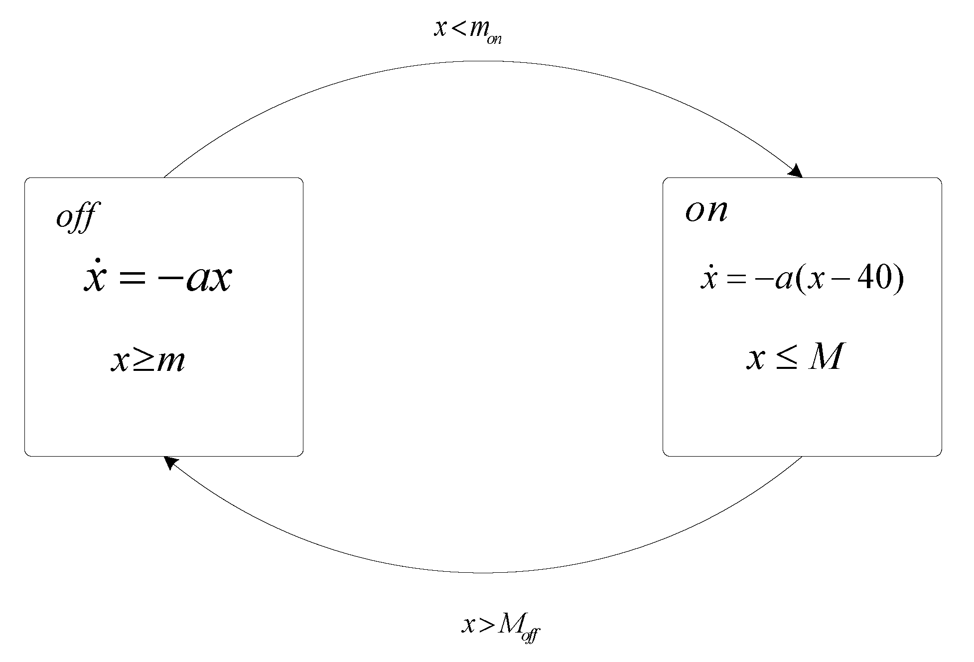
Example 1

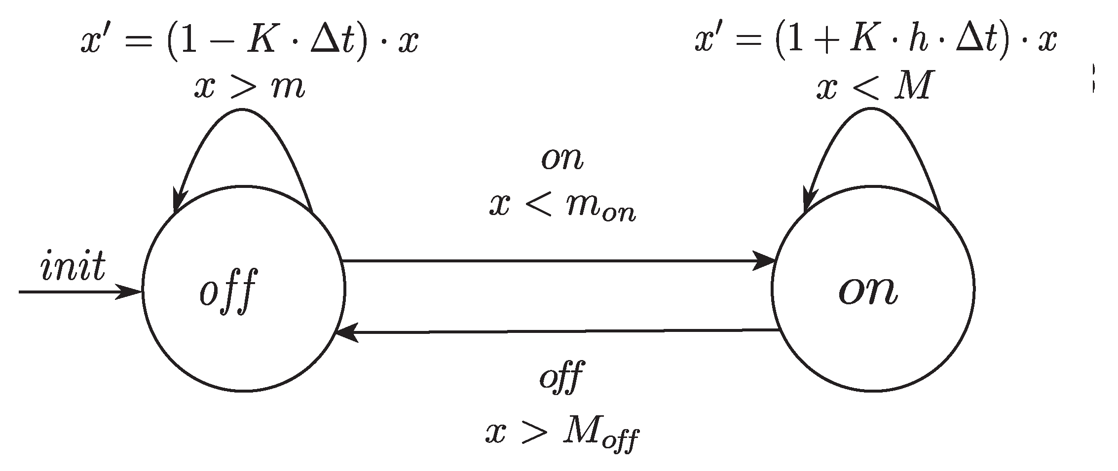
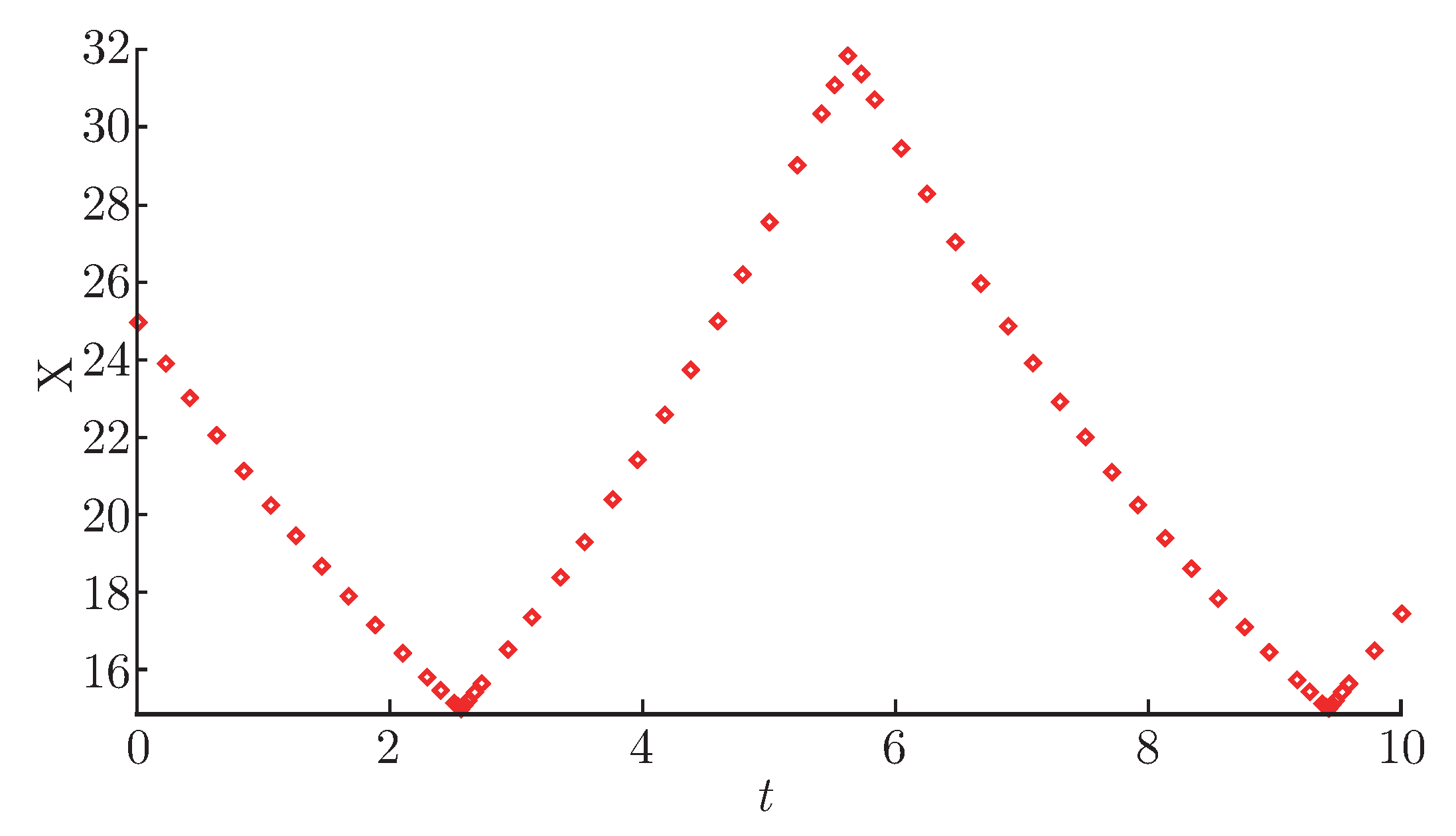
(A thermostat). Consider a room being heated by a radiator controlled by a thermostat, one of the typical introductory examples of hybrid systems. This system has both a continuous state and two discrete states. The continuous state is the temperature in the room $x\in \mathbb{R}$. The discrete states, $L=\{on,off\}$, reflect whether the radiator is on or off. The evolution of x is governed by a differential equation, while the evolution of L is through jumps. It is very convenient to compactly describe such hybrid systems by mixing the differential equation with the directed graph notation (shown in Figure 1).

Computers are used as control systems for a wide variety of industrial and consumer devices. However, the working principle of computers is fundamentally discrete rather than continuous. When the time x is discretized, the general hybrid system (Figure 1) can be turned into an ILAHS(Figure 2), where

$$\left\{\begin{array}{c}L=\{on,off\},\hfill \\ V=\left\{x\right\},\hfill \\ \mathcal{T}=\{〈on,{\alpha }_1,off〉,〈off,{\alpha }_2,on〉\},{\alpha }_{1,2}=\{x^{\prime }=x\},\hfill \\ F(on)=\{x^{\prime }=(1+K.h.\Delta t)x\},\hfill \\ F(off)=\{x^{\prime }=(1-K.\Delta t)x\}.\hfill \end{array}\right.$$

(1)

The ILAHS’ behaviors are expressed as trajectories. For instance, we assume that $m=15$, $m_{on}=20$, $M=32$, $M_{off}=30$, $\Delta t=0.1$, $K=0.2$, and $h=5$. If the initial temperature of the room is ${25}^{ \circ }$C, then one possible trajectory is as follows (Figure 3):

$$\begin{array}{c}〈\mathrm{off},25〉\to 〈\mathrm{off},24.5〉\to 〈\mathrm{off},24.01〉\to \dots \to 〈\mathrm{on},15.09〉\to 〈\mathrm{on},16.60〉\to \dots \hfill \end{array}$$

Definition 4

(Metric). For a set X, a metric on X is a function $d_X:X\times X\mapsto {\mathbb{R}}^{+}$ such that

1. 

for all $x,y\in X,d_X(x,y)=0$ if and only if $x=y$;

2. 

$d_X(x,y)=d_X(y,x)$, for all $x,y\in X$; and

3. 

$d_X(x,z)\le d_X(x,y)+d_X(y,z)$ for all $x,y,z\in X$.

Note that the condition (1) expresses that $d_X(x,y)=0$ implies $x=y$. If $d_X(x,y)=0$ does not necessarily mean that $x=y$, the metric is called a pseudo-metric [12].

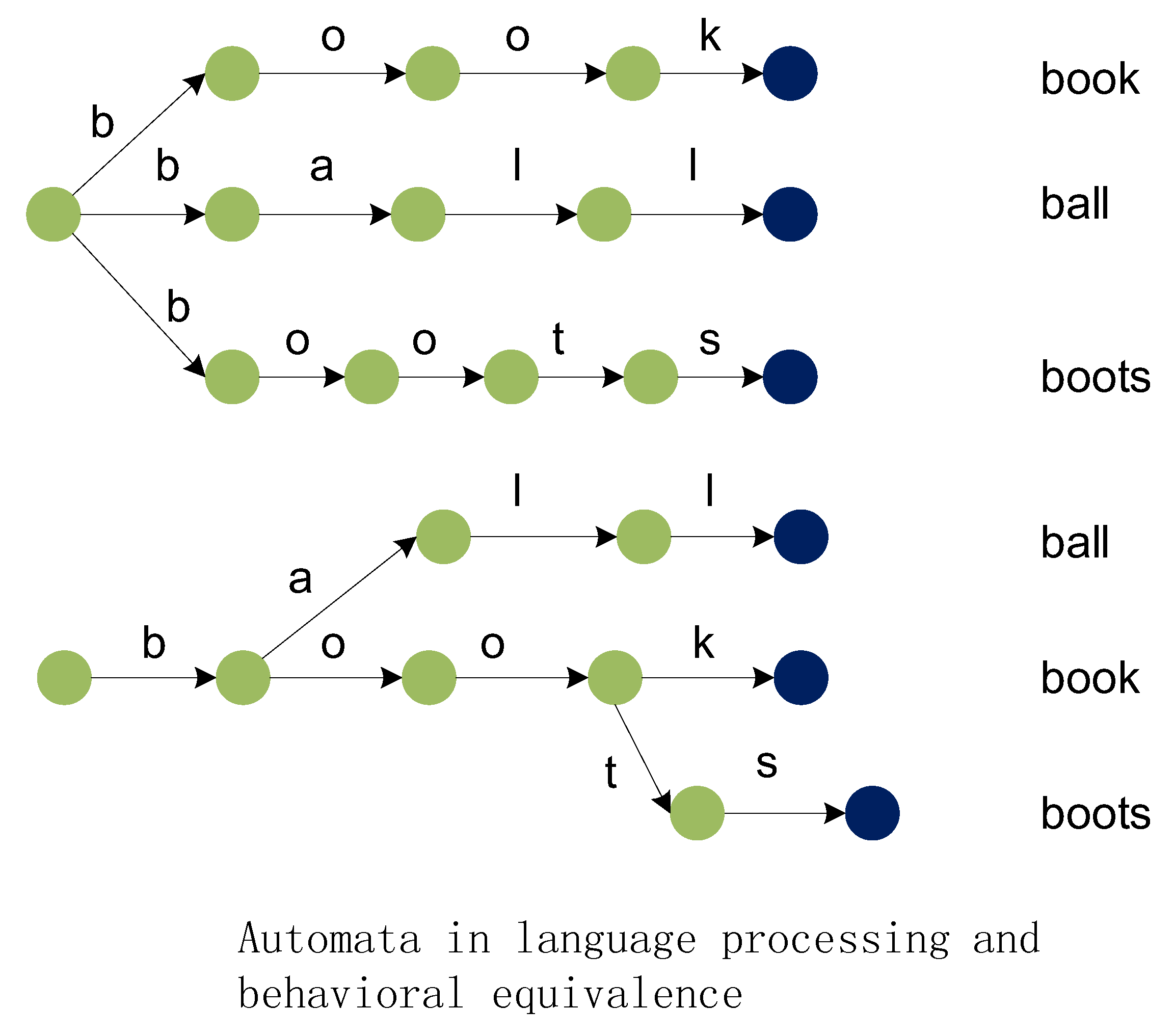
Definition 5

(Trace Equivalence). $\delta \in Ac{t}^{\ast }$ is a trace of a process p, if there exists a process q, such that $p\stackrel{\delta }{⟶}q$. Let $T(p)$ denote the set of traces of p. Two processes p and q are trace equivalent if $T(p)=T(q)$. In trace semantics, two processes are identified iff they are trace equivalent.

Trace semantics is based on the idea that two processes are to be identified if they allow the same set of observations, where an observation simply consists of a sequence of actions performed by the process in succession (Figure 4). More details can be found in the paper [2].

However, $Act$ consists of abstract actions, which are unable to express the exchange details of the data stream. In 2008, Sankaranarayanan et al. [30] defined a hybrid system program model with polynomial equations that took the place of abstract actions and opened up a new method of hybrid system design and verification based on polynomial algebra. For example, the transition ${\ell }_0\stackrel{\alpha }{⟶}{\ell }_1$ with $\alpha \equiv {(x-1)}^2+{(x^{\prime }-2)}^2+{(y^{\prime }-3)}^2=0$ indicates the relation $\left\{〈({\ell }_0,s_0),({\ell }_1,s_1)〉|s_0=(1,y)\wedge s_1=(2,3),y\in \mathbb{R}\right\}$, the variable x refers to the current state, and $x^{\prime }$ to the next state of a transition.

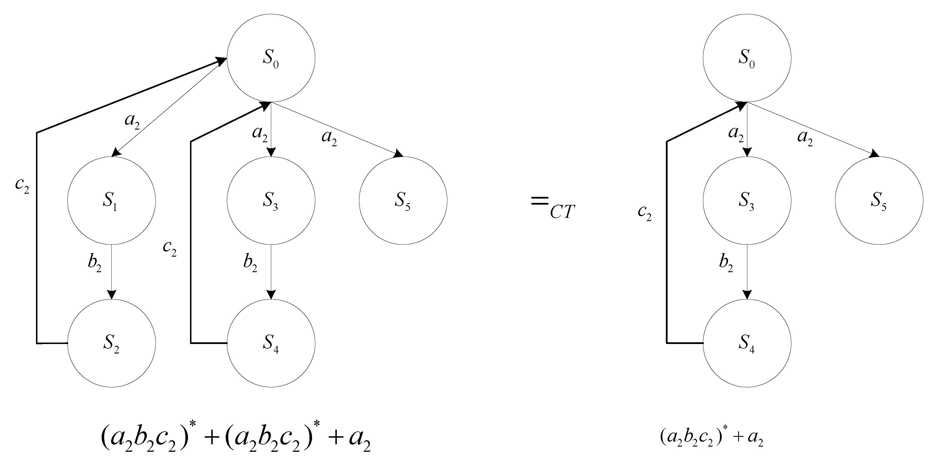
Definition 6

(Completed Trace Equivalence). $\delta \in Ac{t}^{\ast }$ is a completed trace of a process p, if there exists a process q, such that $p\stackrel{\delta }{⟶}q$ and $I(q)=\varnothing$. Let $CT(p)$ denote the set of completed traces of p. Two processes p and q are completed trace equivalent if $T(p)=T(q)$ and $CT(p)=CT(q)$. In completed trace semantics, two processes are identified iff they are completed trace equivalent (Figure 5).

Obviously, the trace equivalence can be regarded as a simpler version of the completed trace equivalence.

Definition 7

(Semi-Algebraic System). A semi-algebraic system (SAS for short) is a conjunctive polynomial formula of the following form:

$$\left\{\begin{array}{c}{p}_1(\overrightarrow{u},\overrightarrow{x})=0,\dots ,p_r(\overrightarrow{u},\overrightarrow{x})=0,\hfill \\ g_1(\overrightarrow{u},\overrightarrow{x})\le 0,\dots ,g_k(\overrightarrow{u},\overrightarrow{x})\le 0,\hfill \\ g_{k+1}(\overrightarrow{u},\overrightarrow{x})>0,\dots ,g_l(\overrightarrow{u},\overrightarrow{x})>0,\hfill \\ h_1(\overrightarrow{u},\overrightarrow{x})\ne 0,\dots ,h_m(\overrightarrow{u},\overrightarrow{x})\ne 0,\hfill \end{array}\right.$$

(2)

where $r\ge 1,l\ge k\ge 0,m\ge 0,\overrightarrow{u}=(u_1,\dots ,u_t),\overrightarrow{x}=(x_1,\dots ,x_r)$, and $p_i,g_i,h_i$ are all in $\mathbb{Q}[\overrightarrow{u},\overrightarrow{x}]\setminus \mathbb{Q}$. An SAS is usually denoted by a quadruple $[\mathbb{P},{\mathbb{G}}_1,{\mathbb{G}}_2,\mathbb{H}]$, where $\mathbb{P}=[p_1,\dots ,p_r],{\mathbb{G}}_1=[g_1,\dots ,g_k],{\mathbb{G}}_2=[g_{k+1},\dots ,g_l]$ and $\mathbb{H}=[h_1,\dots ,h_m]$. An SAS is called parametric if $t\ne 0$, otherwise it is constant.

For $SAS$, what we are concerned about is the real solutions of the equations ($\mathbb{P}$) under the constraints (${\mathbb{G}}_1,{\mathbb{G}}_2,\mathbb{H}$). More specifically, assuming S is a constant $SAS$, the interesting questions are how to compute the number of real solutions of S, and if the number is finite, how to compute these real solutions. Assuming S is parametric $SAS$, the interesting problem is the so-called real solution classification, which is to determine the condition on the parameters such that the system has the prescribed number of distinct real solutions, which is possibly infinite.

To address this issue, Yang et al. [6] first defined the key concept of border polynomial(BP), based on which an algorithm is proposed. For more details, please refer to [7,8,9,10,11]. This algorithm has been improved and implemented by Xia as the Maple package DISCOVERER [31]. Since 2009, the main functions of DISCOVERER have been integrated into the RegularChains library of Maple. Since then, the implementation has been improved by Chen et al. [32,33,34]. Thus, the experiment in this paper requires a version of Maple higher than Maple 13.

Example 2.

Prove that $f\ge 0$ under the constraints $a\ge 0,b\ge 0,c\ge 0,abc-1=0$, i.e.,

$$\left.\begin{array}{c}a\ge 0\hfill \\ b\ge 0\hfill \\ c\ge 0\hfill \\ abc-1=0\hfill \end{array}\right\}\vDash f\ge 0.$$

(3)

In other words,

$$\left\{\begin{array}{cc}a\ge 0\hfill & \\ b\ge 0\hfill & \\ c\ge 0\hfill & \mathrm{has}\mathrm{no}\mathrm{solution}\hfill \\ abc-1=0\hfill & \\ f<0\hfill & \end{array}\right.$$

(4)

where $f=2b^4{c}^4+2b^3{c}^{4}a+2b^4{c}^{3}a+2a^3{c}^3{b}^2+2a^4{c}^{3}b+2a^3{c}^{4}b+2a^4{c}^4+2a^3{b}^{4}c+2a^4{b}^4+2a^3{b}^3{c}^2+2a^4{b}^{3}c-3b^5{c}^4{a}_6^3{b}^4{c}^4{a}^4-3b^5{c}^3{a}^4-3b^4{c}^3{a}^5-3b^4{c}^5{a}^3-3b^3{c}^5{a}^4-3b^3{c}^4{a}^5.$

In order to prove (4) with Maple, we first start Maple and load two relative packages of RegularChains as follows.

•     > with (RegularChains):
•     > with (ParametricSystemTools):
•     > with (SemiAlgebraicSetTools):
• Then we define an order of the unknowns:
•     > R:= PolynomialRing ([a, b, c]):
• Then, by calling
•     >RealRootClassification ([abc-1], [a,b,c], [-f], [ ], 2, 0, R):

we will know at once that the inequality holds.

3. $\mathit{\epsilon }$-Approximate Completed Trace Equivalence of ILAHS

In this section, we define $\epsilon$-approximate completed trace equivalence of ILAHS and propose the discriminant conditions based on SAS. Assuming $\mathcal{H}$ is an ILAHS and $\mathfrak{T}$ is a trajectory of $\mathcal{H}$,

$$〈{\ell }_0,{\widehat{\overrightarrow{v}}}_{00}〉\stackrel{A_0}{⟶}〈{\ell }_0,{\widehat{\overrightarrow{v}}}_{01}〉\stackrel{A_0}{⟶}\cdots 〈{\ell }_0,{\widehat{\overrightarrow{v}}}_{0m_0}〉\stackrel{la{b}_{01}}{⟶}〈{\ell }_1,{\widehat{\overrightarrow{v}}}_{10}〉,\dots ,\stackrel{A_n}{⟶}〈{\ell }_n,{\widehat{\overrightarrow{v}}}_{n0}〉,\dots .$$

$A_i$ is an original (or theoretical) transition matrix, $la{b}_{01}$ is discrete evolution, for simplicity, $la{b}_{01}:v_i^{\prime }=v_i$, and so on. ${\tilde{A}}_i$ is an approximate (or actual) matrix with respect to $A_i$, so we have another trajectory,

$$〈{\ell }_0,{\widetilde{\widehat{\overrightarrow{v}}}}_{00}〉\stackrel{{\tilde{A}}_0}{⟶}〈{\ell }_0,{\widetilde{\widehat{\overrightarrow{v}}}}_{01}〉\stackrel{{\tilde{A}}_0}{⟶}\cdots 〈{\ell }_0,{\widetilde{\widehat{\overrightarrow{v}}}}_{0m_0}〉\stackrel{la{b}_{01}}{⟶}〈{\ell }_1,{\widetilde{\widehat{\overrightarrow{v}}}}_{10}〉,\dots ,\stackrel{{\tilde{A}}_n}{⟶}〈{\ell }_n,{\widetilde{\widehat{\overrightarrow{v}}}}_{n0}〉,\dots .$$

If a given derivation $\epsilon$ is allowable, we aim to check whether two trajectories are identical; if every trajectory of two ILAHSs is identical, the two hybrid systems are identical with respect to derivation $\epsilon$.

To measure the behavior of the hybrid system, this paper defines two types of metrics based on the Euclidean metric: the state metric $d_{sta}$ and the trajectory metric $d_{trj}$. $d_{sta}$ measures the distance of states, while $d_{trj}$ specifies the similarity of two systems’ behaviors.

Definition 8

(State Metric). State metric $d_{sta}$ is Euclidean metric: ${\mathbb{R}}^n\times {\mathbb{R}}^n\to [0,1]$ such that

$$\begin{array}{cc}\hfill d_{sta}\left(〈l,\widehat{\overrightarrow{v}}〉,〈l^{\prime },\widetilde{\widehat{\overrightarrow{v}}}〉\right)& =\left\{\begin{array}{cc}1\hfill & \hfill ifl\ne l^{\prime },\\ d_e\left(\widehat{\overrightarrow{v}},\widetilde{\widehat{\overrightarrow{v}}}\right)\hfill & \hfill ifl=l^{\prime },\end{array}\right.\hfill \\ \hfill & \mathit{where}{d}_e\left(\widehat{\overrightarrow{v}},\widetilde{\widehat{\overrightarrow{v}}}\right)=\frac{\sqrt{{\displaystyle \sum _{i=1}^n}{({\widehat{v}}_i-{\tilde{\widehat{v}}}_i)}^2}}{1+\sqrt{{\displaystyle \sum _{i=1}^n}{({\widehat{v}}_i-{\tilde{\widehat{v}}}_i)}^2}}.\hfill \end{array}$$

(5)

If $l=l^{\prime }$, $d_{sta}\left(〈l,\widehat{\overrightarrow{v}}〉,〈l^{\prime },\widetilde{\widehat{\overrightarrow{v}}}〉\right)$ can be abbreviated as $d_{sta}\left(\widehat{\overrightarrow{v}},\widetilde{\widehat{\overrightarrow{v}}}\right)$.

Definition 9

(Trajectory Metric). Trajectory metric $d_{trj}$ is defined as the minimum distance of relevant states, i.e.,

$$d_{trj}({\mathfrak{T}}_1,{\mathfrak{T}}_2)=\begin{array}{c}min\left(d_{sta}\left(〈l,{\widehat{\overrightarrow{v}}}_i〉,〈l,\tilde{{\widehat{\overrightarrow{v}}}_i}〉\right)\right).\hfill \end{array}$$

(6)

Definition 10

($\epsilon$-Approximate States). Given a deviation ε, $〈l,\widehat{\overrightarrow{v}}〉$ is ε-approximate to $〈l^{\prime },\widetilde{\widehat{\overrightarrow{v}}}〉$ iff $d_{sta}\left(〈l,\widehat{\overrightarrow{v}}〉,〈l^{\prime },\widetilde{\widehat{\overrightarrow{v}}}〉\right)\le \epsilon$.

Definition 11

($\epsilon$-Approximate Trajectories). Given a deviation ε and two trajectories ${\mathfrak{T}}_1$ and ${\mathfrak{T}}_2$, ${\mathfrak{T}}_1$ is ε-approximate to ${\mathfrak{T}}_2$ iff $d_{trj}({\mathfrak{T}}_1,{\mathfrak{T}}_2)\le \epsilon$.

Definition 12

($\epsilon$-Approximate Completed Trace Equivalence of ILAHS). Given a deviation ε, if all completed traces of two ILAHSs are ε-approximate trajectories, then the two ILAHSs are ε-approximate completed trace equivalence.

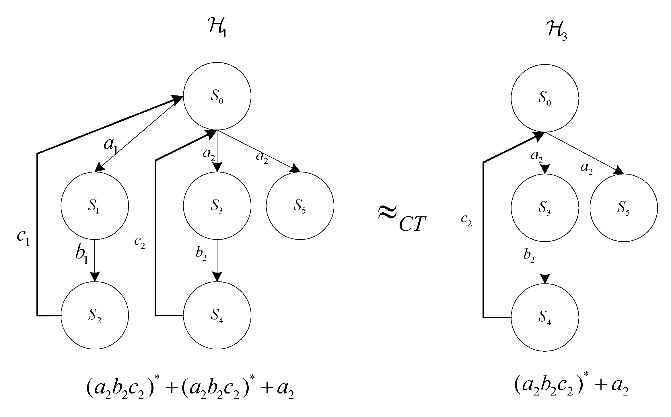
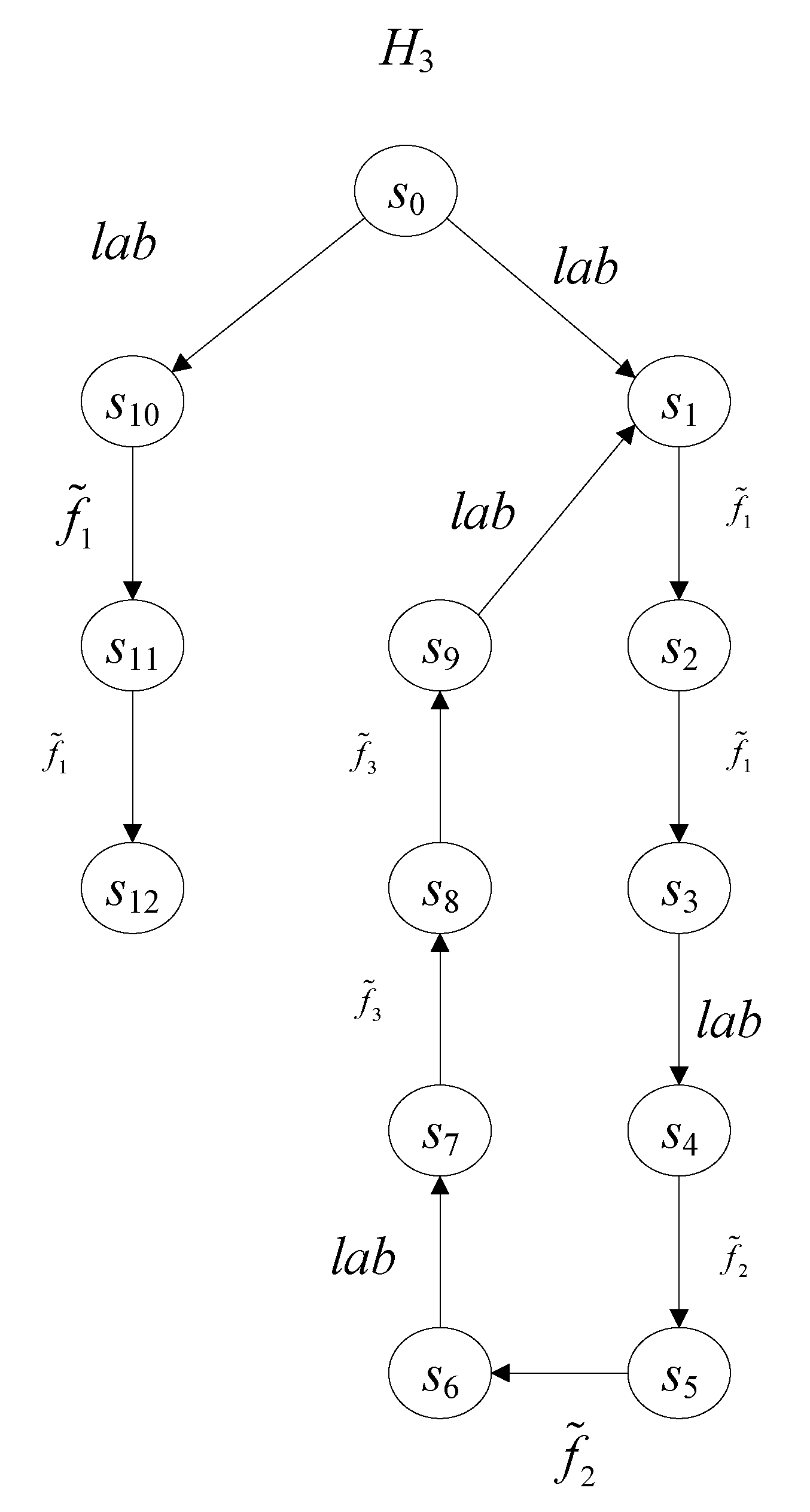
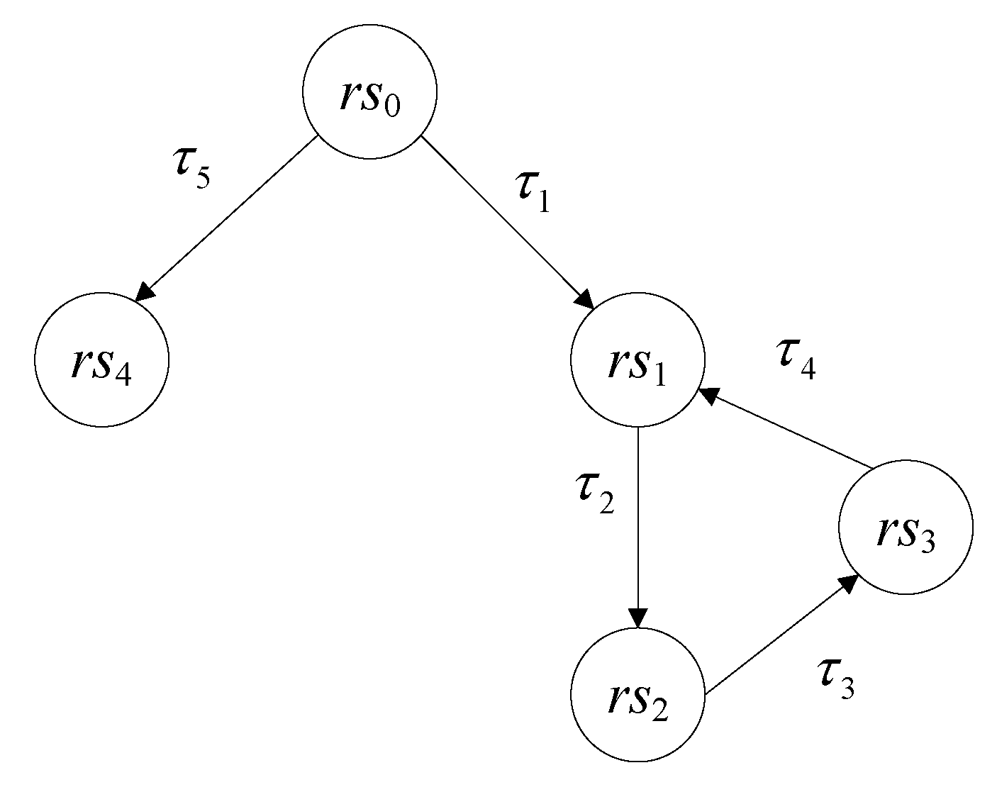
In Figure 6, ${\mathcal{H}}_1$ is an original ILAHS, given a deviation $\epsilon$, ${\mathcal{H}}_1$ and ${\mathcal{H}}_3$ are completed trace equivalence, in the semantics of completed trace equivalence, ${\mathcal{H}}_3$ is identical to ${\mathcal{H}}_1$.

Obviously, ${\mathcal{H}}_3$ involves fewer states than ${\mathcal{H}}_1$; in other words, by approximate completed trace equivalence, the research on hybrid systems can be simplified.

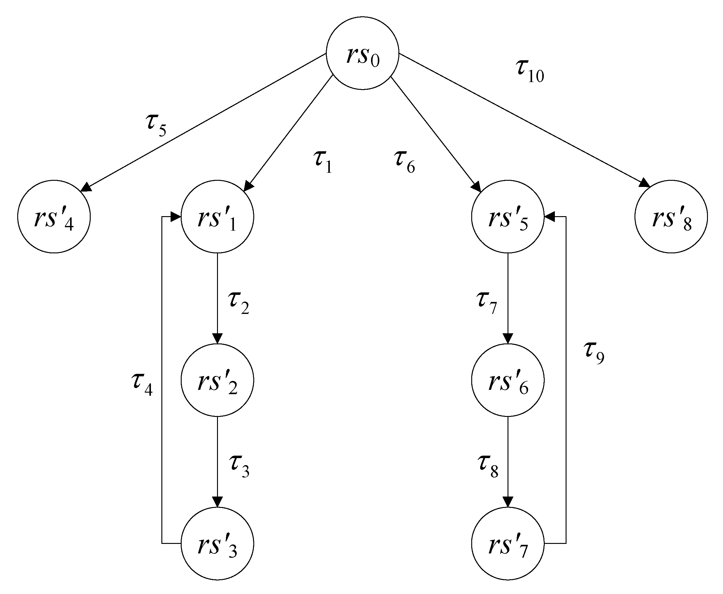
Since there exist two categories of trajectories in completed trace equivalence (Figure 6), the infinite trajectory ${(a_2{b}_2{c}_2)}^{\ast }$ and the finite trajectory $a_2$, there are two corresponding decision conditions, the finite trajectory condition and the infinite trajectory condition. For simplicity, assume discrete evolution such as $la{b}_{01}:v_i^{\prime }=v_i$.

Definition 13

(Finite Trajectory Condition). For a finite trajectory ${\mathfrak{T}}_{\mathfrak{1}}$

$$〈{\ell }_0,{\widehat{\overrightarrow{v}}}_{00}〉\stackrel{A_0}{⟶}〈{\ell }_0,{\widehat{\overrightarrow{v}}}_{01}〉\stackrel{A_0}{⟶}\cdots 〈{\ell }_0,{\widehat{\overrightarrow{v}}}_{0m_0}〉\stackrel{la{b}_{01}}{⟶}〈{\ell }_1,{\widehat{\overrightarrow{v}}}_{10}〉,\dots ,\stackrel{A_n}{⟶}〈{\ell }_n,{\widehat{\overrightarrow{v}}}_{n{m}_n}〉.$$

such that

$$\left\{\begin{array}{cc}{\widehat{\overrightarrow{v}}}_{00}\hfill & \in \mathsf{\Theta }\hfill \\ \overrightarrow{v}\hfill & ={\widehat{\overrightarrow{v}}}_{00}\hfill \\ \tilde{\overrightarrow{v}}\hfill & ={\widehat{\overrightarrow{v}}}_{00}\hfill \\ {\overrightarrow{v}}^{\prime }\hfill & =(A_0^{m_0}{A}_1^{m_1}\dots A_i^{m_i})\overrightarrow{v}\hfill & \mathit{have}\mathit{no}\mathit{solution}\mathit{for}\mathit{every}0\le i\le n.\hfill \\ {\tilde{\overrightarrow{v}}}^{\prime }\hfill & =({\tilde{A}}_0^{m_0}{\tilde{A}}_1^{m_1}\dots {\tilde{A}}_i^{m_i})\tilde{\overrightarrow{v}}\hfill \\ d_{sta}({\overrightarrow{v}}^{\prime },{\tilde{\overrightarrow{v}}}^{\prime })\hfill & >\epsilon \hfill \end{array}\right.$$

(7)

The infinite trajectory condition is defined by the inductive method.

Definition 14

(Infinite Trajectory Condition). For an infinite trajectory ${\mathfrak{T}}_{\mathfrak{2}}$

$$〈{\ell }_0,{\widehat{\overrightarrow{v}}}_{00}〉\stackrel{A_0}{⟶}〈{\ell }_0,{\widehat{\overrightarrow{v}}}_{01}〉\stackrel{A_0}{⟶}\cdots 〈{\ell }_0,{\widehat{\overrightarrow{v}}}_{0m_0}〉\stackrel{la{b}_{01}}{⟶}〈{\ell }_1,{\widehat{\overrightarrow{v}}}_{10}〉,\dots ,\stackrel{A_n}{⟶}〈{\ell }_n,{\widehat{\overrightarrow{v}}}_{n{m}_n}〉\stackrel{la{b}_{n0}}{⟶}〈{\ell }_0,{\widehat{\overrightarrow{v}}}_{{00}^{\prime }}〉\stackrel{A_0}{⟶}\cdots ,$$

such that

$$Initiation:\left\{\begin{array}{c}\overrightarrow{v},\tilde{\overrightarrow{v}}\in \mathsf{\Theta }\hfill \\ d_{sta}(\overrightarrow{v},\tilde{\overrightarrow{v}})>\epsilon \hfill \end{array}\right.$$

(8)

$$Consecution:\left\{\begin{array}{cc}{\overrightarrow{v}}^{\prime }\hfill & =(A_0^{m_0}{A}_1^{m_1}\dots A_i^{m_i})\overrightarrow{v}\hfill \\ {\tilde{\overrightarrow{v}}}^{\prime }\hfill & =({\tilde{A}}_0^{m_0}{\tilde{A}}_1^{m_1}\dots {\tilde{A}}_i^{m_i})\tilde{\overrightarrow{v}}\hfill \\ d_{sta}({\overrightarrow{v}}^{\prime },{\tilde{\overrightarrow{v}}}^{\prime })\hfill & >\epsilon \hfill \end{array}\right.$$

(9)

for every $0\le i\le n$, (8) and (9) have no solution.

The condition Initiation shows that the deviation of two states is initially less than $\epsilon$; the condition Consecution shows that deviation less than $\epsilon$ is preserved by the loop.

Complexity Analysis: Take (9) for example. Assuming $\overrightarrow{v}=\{v_1,v_2,\dots v_n\}$, $deg(v_i)\le 2,1\le i\le n$, our method consists of three main steps. In the first step, we transform the equations of (9) into triangular sets (i.e., equations in the triangular form) by Ritt–Wu’s method. By [35], the complexity of this step is $\mathcal{O}({(2n)}^{{(2n)}^{\mathcal{O}(1)}}{(2+1)}^{{\mathcal{O}}^{{(2n)}^3}})$. The second step is to compute a border polynomial (BP) from the triangularized systems through resultant computation. By [35], the complexity of computing the BP is at most $(2n+2)\mathcal{O}({(2n)}^{6n+2n^2}{(2+1)}^{2n^3})$. Finally, we use the PCAD(partial cylindrical algebraic decomposition) algorithm with the BP to obtain the real solution classification; the complexity of this step is at most $\mathcal{O}(2D^{2^{4n+8}})$, where $D=\mathcal{O}({(2n)}^{4n^2+8n^3}{(2+1)}^{4n^3})$, the highest degree of BP.

A Special Case: The approaches proposed in papers [4,5,24] use the Frobenius norm to study approximate equivalence of real-time linear algebraic hybrid automaton. Their approaches can only apply to a class of special matrices. We now prove that their approaches are a special case of our approach.

We first introduce the conclusions in their papers [4,5,24].

For $A_j$ and its approximate matrix ${\tilde{A}}_j=A+{\delta }_{A_j}$, which are $n\times n$ nonsingular matrices, the eigenvalues of matrix A are ${\lambda }_i(i=1,\dots ,n)\in \mathbb{R}$, and there exists an orthogonal matrix U:

$$\begin{array}{cc}\hfill & A_k=U^T\left[\begin{array}{ccc}{\lambda }_{k1}& & \ast \\ & \ddots \\ & & {\lambda }_{kn}\end{array}\right]U,\hfill \\ \hfill & A_k+{\delta }_{A_k}=U^T\left[\begin{array}{ccc}{\lambda }_{k1}+{\delta }_{{\lambda }_{k1}}& & \ast \\ & \ddots \\ & & {\lambda }_{kn}+{\delta }_{{\lambda }_{kn}}\end{array}\right]U,\hfill \\ \hfill & A_k{A}_{k-1}\dots A_1=U^T\left[\begin{array}{cc}{\lambda }_{11}\dots {\lambda }_{k1}& \ast \\ & \ddots \\ & {\lambda }_{1n}\dots {\lambda }_{kn}\end{array}\right]U,\hfill \\ \hfill & (A_k+{\delta }_{A_k})(A_{k-1}+{\delta }_{A_{k-1}})\dots (A_1+{\delta }_{A_1})=U^T\left[\begin{array}{ccc}({\lambda }_{11}+{\delta }_{{\lambda }_{11}})\dots ({\lambda }_{k1}+{\delta }_{{\lambda }_{k1}})& & \ast \\ & \ddots \\ & & ({\lambda }_{1n}+{\delta }_{{\lambda }_{1n}})\dots ({\lambda }_{kn}+{\delta }_{{\lambda }_{kn}})\end{array}\right]U,\hfill \\ \hfill & {\delta }_{A_j}={\tilde{A}}_j-A_j,{\parallel {\delta }_{A_j}\parallel }_2=r_j{\parallel A_j\parallel }_2,\hfill \\ \hfill & {\delta }_k=(A_k+{\delta }_{A_k})(A_{k-1}+{\delta }_{A_{k-1}})\dots (A_1+{\delta }_{A_1})-A_k{A}_{k-1}\dots A_1\hfill \\ \hfill & \le ((1+r_1)\dots (1+r_k)-1){\parallel A_1\parallel }_2\cdots {\parallel A_k\parallel }_2\hfill \\ \hfill & \le (e^{r_1+r_2\dots +r_k}-1){\parallel A_1\parallel }_2{\parallel A_2\parallel }_2\cdots {\parallel A_k\parallel }_2=W_k.\hfill \end{array}$$

Then, for a deviation $\omega$ and $\frac{W_k}{{\parallel A_k{A}_{k-1}\dots A_1\parallel }_2}\le \omega$, if $A_k{A}_{k-1}\dots A_1$ are $\omega$-approximate to $(A_k+{\delta }_{A_k})(A_{k-1}+{\delta }_{A_{k-1}})\dots (A_1+{\delta }_{A_1})$, $\forall h\in N^{+}$ and $1\le h<k$, $A_h{A}_{h-1}\dots A_1$ are $\omega$-approximate to $(A_h+{\delta }_{A_h})(A_{h-1}+{\delta }_{A_{h-1}})\dots (A_1+{\delta }_{A_1})$.

This conclusion is equivalent to (11) ⊧ (13) for an existing constant $\epsilon$.

Proof. 

$$\begin{array}{cc}\hfill \because d_{sta}^{(k)}({\overrightarrow{v}}^{\prime },{\tilde{\overrightarrow{v}}}^{\prime })& =\parallel ({\tilde{A}}_1{\tilde{A}}_2\dots {\tilde{A}}_k-A_1{A}_2\dots A_k){\widehat{\overrightarrow{v}}}_0{\parallel }_2\hfill \\ \hfill & =\parallel {\delta }_k{\widehat{\overrightarrow{v}}}_0{\parallel }_2\le \parallel {\delta }_k{\parallel }_2\parallel {\widehat{\overrightarrow{v}}}_0{\parallel }_2\le W_k{\parallel {\widehat{\overrightarrow{v}}}_0\parallel }_2\hfill \\ \hfill & \le \omega {\parallel A_k{A}_{k-1}\dots A_1\parallel }_2{\parallel {\widehat{\overrightarrow{v}}}_0\parallel }_2=\epsilon ,\hfill \end{array}$$

(10)

∴

$$\left\{\begin{array}{cc}{\widehat{\overrightarrow{v}}}_0\hfill & \in \mathsf{\Theta }\hfill \\ \overrightarrow{v}\hfill & ={\widehat{\overrightarrow{v}}}_0\hfill \\ \tilde{\overrightarrow{v}}\hfill & ={\widehat{\overrightarrow{v}}}_0\hfill & \mathrm{has}\mathrm{no}\mathrm{solution},\hfill \\ {\overrightarrow{v}}^{\prime }\hfill & =(A_1{A}_2\dots A_k)\overrightarrow{v}\hfill \\ {\tilde{\overrightarrow{v}}}^{\prime }\hfill & =({\tilde{A}}_1{\tilde{A}}_2\dots {\tilde{A}}_k)\tilde{\overrightarrow{v}}\hfill \\ d_{sta}^{(k)}({\overrightarrow{v}}^{\prime },{\tilde{\overrightarrow{v}}}^{\prime })\hfill & >\epsilon \hfill \end{array}\right.$$

(11)

$$\begin{array}{cc}\hfill and\because d_{sta}^{(h)}({\overrightarrow{v}}^{\prime },{\tilde{\overrightarrow{v}}}^{\prime })& =\parallel ({\tilde{A}}_1{\tilde{A}}_2\dots {\tilde{A}}_h-A_1{A}_2\dots A_h){\widehat{\overrightarrow{v}}}_0{\parallel }_2\hfill \\ \hfill & =\parallel {\delta }_h{\widehat{\overrightarrow{v}}}_0{\parallel }_2\le \parallel {\delta }_h{\parallel }_2{\parallel {\widehat{\overrightarrow{v}}}_0\parallel }_2\hfill \\ \hfill & \le ((1+r_1)(1+r_2)\dots (1+r_h)-1){\parallel A_1\parallel }_2{\parallel A_2\parallel }_2\cdots {\parallel A_h\parallel }_2{\parallel {\widehat{\overrightarrow{v}}}_0\parallel }_2\hfill \\ \hfill & \le ((1+r_1)(1+r_2)\dots (1+r_h)\dots (1+r_k)-1){\parallel A_1\parallel }_2{\parallel A_2\parallel }_2\cdots {\parallel A_k\parallel }_2{\parallel {\widehat{\overrightarrow{v}}}_0\parallel }_2\hfill \\ \hfill & \le W_k\parallel {\widehat{\overrightarrow{v}}}_0{\parallel }_2\le \omega {\parallel A_k{A}_{k-1}\dots A_1\parallel }_2{\parallel {\widehat{\overrightarrow{v}}}_0\parallel }_2=\epsilon ,\hfill \end{array}$$

(12)

i.e., for every $1\le h<k$,

$$\left\{\begin{array}{cc}{\widehat{\overrightarrow{v}}}_0\hfill & \in \mathsf{\Theta }\hfill \\ \overrightarrow{v}\hfill & ={\widehat{\overrightarrow{v}}}_0\hfill \\ \tilde{\overrightarrow{v}}\hfill & ={\widehat{\overrightarrow{v}}}_0\hfill & \mathrm{has}\mathrm{no}\mathrm{solution},\hfill \\ {\overrightarrow{v}}^{\prime }\hfill & =(A_1{A}_2\dots A_h)\overrightarrow{v}\hfill \\ {\tilde{\overrightarrow{v}}}^{\prime }\hfill & =({\tilde{A}}_1{\tilde{A}}_2\dots {\tilde{A}}_h)\tilde{\overrightarrow{v}}\hfill \\ d_{sta}^{(h)}({\overrightarrow{v}}^{\prime },{\tilde{\overrightarrow{v}}}^{\prime })\hfill & >\epsilon \hfill \end{array}\right.$$

(13)

in other words, (11) ⊧ (13). □

4. Experiments

In this section, we present an example to demonstrate the application of our method to simplify the ILAHS in approximate completed trace equivalence semantics. Figure 7 is a boiler feed-water control system, which has both continuous and discrete states and can be modeled as a hybrid system. For simplicity, we assume that there exist nine discrete locations that are divided according to the combination of fuel supply (low, high) and outdoor temperature (low, medium, high). $r{s}_0$ is the initial location of the system, which does not involve continuous evolution and directly jumps to a different location by ${\tau }_i$. The continuous variables $X={(x_1,x_2)}^T$; $x_1$ and $x_2$ stand for water level and water supply, respectively. The fuel supply and outdoor temperature have an effect on $x_1$ and $x_2$, and the regulation rules of $x_1$ and $x_2$ conform to their respective differential equations at different locations $r{s}_i^{\prime }(i=1,\dots ,8)$. The initial state of the system $X_0={(100,10)}^T$, and for ${\tau }_i$, the discrete transition program ${\alpha }_i:x_1^{\prime }=x_1\wedge x_2^{\prime }=x_2$, labeled by $lab$. Assuming the duration time at every location $r{s}_i^{\prime }(i=1,\dots ,8)$ is 10 s and the discrete time of continuous evolution is 5 s, Figure 8 is the corresponding ILAHS.

$$\begin{array}{ccc}{f}_1,f_4:\hfill & X^{\prime }=\left[\begin{array}{cc}\frac{111}{100}& \frac{2}{5}\\ 0& \frac{151}{100}\end{array}\right]X{f}_8,f_5:\hfill & X^{\prime }=\left[\begin{array}{cc}\frac{109}{100}& \frac{2}{5}\\ 0& \frac{149}{100}\end{array}\right]X\hfill \\ f_2:\hfill & X^{\prime }=\left[\begin{array}{cc}\frac{111}{100}& \frac{11}{111}\\ 0& 1\end{array}\right]X{f}_3:\hfill & X^{\prime }=\left[\begin{array}{cc}1& -\frac{51}{151}\\ 0& \frac{100}{151}\end{array}\right]X\hfill \\ f_6:\hfill & X^{\prime }=\left[\begin{array}{cc}\frac{100}{109}& \frac{9}{109}\\ 0& 1\end{array}\right]X{f}_7:\hfill & X^{\prime }=\left[\begin{array}{cc}1& -\frac{49}{149}\\ 0& \frac{100}{149}\end{array}\right]X\hfill \end{array}$$

The original invariant set is

$$\begin{array}{cc}Inv(r{s}_1^{\prime }):\hfill & \{(100\le x_1\le 133.69)\wedge (10\le x_2\le 22.801)\},\hfill \\ Inv(r{s}_2^{\prime }):\hfill & \{(112.801\le x_1\le 133.69)\wedge (x_2=22.801)\},\hfill \\ Inv(r{s}_3^{\prime }):\hfill & \{(100\le x_1\le 112.801)\wedge (10\le x_2\le 22.801)\},\hfill \\ Inv(r{s}_4^{\prime }):\hfill & \{(100\le x_1\le 133.69)\wedge (10\le x_2\le 22.801)\},\hfill \\ Inv(r{s}_5^{\prime }):\hfill & \{(100\le x_1\le 129.13)\wedge (10\le x_2\le 22.201)\},\hfill \\ Inv(r{s}_6^{\prime }):\hfill & \{(112.801\le x_1\le 129.13)\wedge (x_2=22.201)\},\hfill \\ Inv(r{s}_7^{\prime }):\hfill & \{(100\le x_1\le 112.201)\wedge (10\le x_2\le 22.201)\},\hfill \\ Inv(r{s}_8^{\prime }):\hfill & \{(100\le x_1\le 129.13)\wedge (10\le x_2\le 22.201)\}.\hfill \end{array}$$

Assume Figure 9 is the approximate ILAHS, where

$$\begin{array}{cc}{\tilde{f}}_1,{\tilde{f}}_4,{\tilde{f}}_5,{\tilde{f}}_8:\hfill & {\tilde{X}}^{\prime }=\left[\begin{array}{cc}\frac{11}{10}& \frac{2}{5}\\ 0& \frac{3}{2}\end{array}\right]X,\hfill \\ {\tilde{f}}_2,{\tilde{f}}_6:\hfill & {\tilde{X}}^{\prime }=\left[\begin{array}{cc}\frac{10}{11}& \frac{1}{11}\\ 0& 1\end{array}\right]X,\hfill \\ {\tilde{f}}_3,{\tilde{f}}_7:\hfill & {\tilde{X}}^{\prime }=\left[\begin{array}{cc}1& -\frac{1}{3}\\ 0& \frac{2}{3}\end{array}\right]X.\hfill \end{array}$$

The approximate invariant set is

$$\begin{array}{cc}\widetilde{Inv(r{s}_1^{\prime })},\widetilde{Inv(r{s}_4^{\prime })}:\hfill & \{(100\le x_1\le 131.4)\wedge (10\le x_2\le 22.5)\},\hfill \\ \widetilde{Inv(r{s}_5^{\prime })},\widetilde{Inv(r{s}_8^{\prime })}:\hfill & \{(100\le x_1\le 131.4)\wedge (10\le x_2\le 22.5)\},\hfill \\ \widetilde{Inv(r{s}_2^{\prime })},\widetilde{Inv(r{s}_6^{\prime })}:\hfill & \{(112.5\le x_1\le 131.4)\wedge (x_2=22.5)\},\hfill \\ \widetilde{Inv(r{s}_3^{\prime })},\widetilde{Inv(r{s}_7^{\prime })}:\hfill & \{(100\le x_1\le 112.5)\wedge (10\le x_2\le 22.5)\}.\hfill \end{array}$$

The approximate discrete transition program is ${\tilde{\alpha }}_i:x_1^{\prime }=x_1\wedge x_2^{\prime }=x_2$, labeled by $lab$.

Given an error derivation $\epsilon =0.1$, ${\mathcal{H}}_1$ is $\epsilon$-approximate completed trace equivalent to ${\mathcal{H}}_3$ (Figure 9), i.e., in the semantics of completed trace equivalence, ${\mathcal{H}}_1$ is identical to ${\mathcal{H}}_3$, which involves fewer states. Therefore, the original hybrid automaton (Figure 7) can be reduced to an equivalent but simpler hybrid automaton (Figure 10), and the design of the hybrid system is optimized with the theory of approximate completed trace equivalence.

5. Conclusions

With some restrictions, a general hybrid system can be specialized into an inhomogeneous linear algebraic hybrid system (ILAHS), which is ubiquitous in reality. Since errors are inevitable in engineering technology, it is meaningful to introduce deviation to the analysis of hybrid systems. Given an error derivation, this paper first proposes the theory of approximate completed trace equivalence. Then we come up with a new approach (based on SAS solving) to approximate completed trace equivalence, and the computation complexity is also analyzed. Finally, a case study is presented to illustrate the practicality of our method. Compared to the well-established approaches in this field, our method applies to more general ILAHS. Moreover, this technology is promising for solving parametric approximate completed trace equivalence. We will address this issue in future work.