Wideband Spectrum Sensing Method Based on Channels Clustering and Hidden Markov Model Prediction


Abstract
1. Introduction
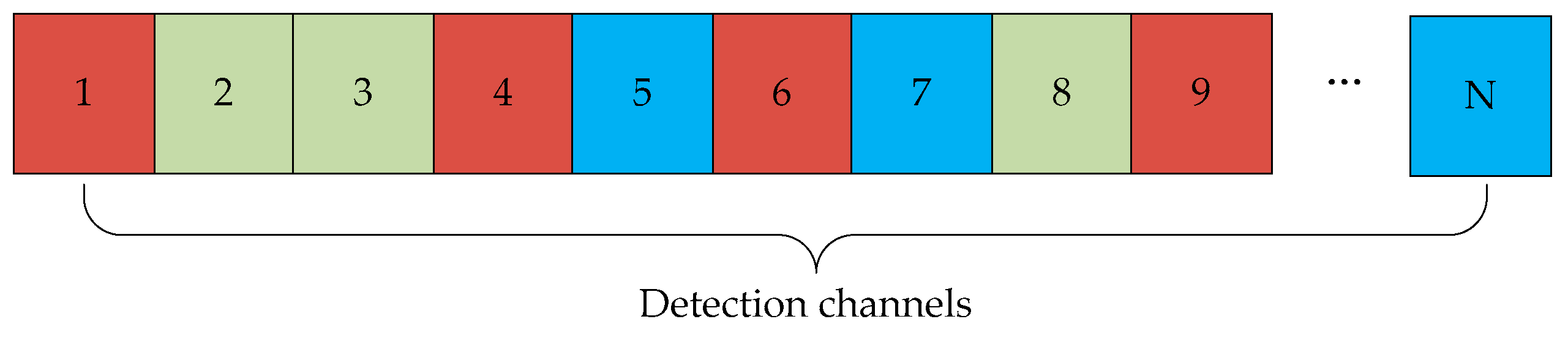
2. System Model
3. Correlation-Based Channels Clustering
3.1. Channel Correlation Metrics
3.2. Channel Correlation Verification
3.3. OPTICS Algorithm for Channel Clustering
| Algorithm 1 Channels clustering algorithm of OPTICS |
| Input: specify channel set to be clustered Parameters: ε and MinPts Output: result queue 1: Create a result queue and a seed queue . 2: Randomly select an unprocessed core object from the channel set and add to , then take the ε-neighborhood channels of object , which is showed as . If the objects of is not in , add to , and then is arranged in ascending order according to the reachability-distance. 3: Select a core object with the smallest reachability-distance in and add to , then take the ε-neighborhood channels of object , which is showed as . If the objects of is in , repeat step 3. Otherwise, go to step 4. 4: if the objects of is already in , the objects of in are arranged in ascending order according to the reachability-distance, and then return to step 3. Otherwise, add to and is arranged in ascending order according to the reachability-distance, then return to step 3. 5: If is empty, return to step 2. 6: If the channel set is empty, the algorithm ends, and the ordered sample objects in the result queue are output. |
3.4. DC Selection and Clustering Results
| Algorithm 2 Obtaining the clustering channels |
| Input: result queue Output: clustered channels 1: Set the threshold radius ε1. 2: Take out the head element of queue . If the reachability-distance of is greater than ε1, add to the current cluster; otherwise, if the core-distance of is less than ε1, add to a new cluster. 3: Repeat step 2 until is empty. 4: The algorithm is end when is empty. |
4. HMM-Based Channel Prediction
4.1. Esimation Model
- represents the initial probability distribution of the state, where , .
- The state transition probability matrix is , where , , and , indicates the state of the model in the time slot of .
- The observation matrix is , where , , and , indicates the observation state of the model in the time slot .
4.2. HMM-Based Channel Prediction
5. Simulation Results and Discussion
5.1. Simulation Results of Channels Clustering
5.2. Performance Analysis
5.3. Performance Comparison
6. Conclusions
Author Contributions
Funding
Acknowledgments
Conflicts of Interest
References
- Mitola, J.; Maguire, G.Q., Jr. Cognitive Radio: Making Software Radios More Personal. IEEE Pers. Commun. 1999, 6, 13–18. [Google Scholar] [CrossRef]
- Chen, Y.F.; Oh, H.S. A Survey of Measurement-based Spectrum Occupancy Modeling for Cognitive Radios. IEEE Commun. Surv. Tutor. 2016, 18, 848–859. [Google Scholar] [CrossRef]
- Hattab, G.; Ibnkahla, M. Multiband Spectrum Access: Great Promises for Future Cognitive Radio Networks. Proc. IEEE 2014, 102, 282–306. [Google Scholar] [CrossRef]
- Ma, Y.; Gao, Y.; Cavallaro, A.; Parini, C.G.; Zhang, W.; Liang, Y.C. Sparsity Independent Sub-Nyquist Rate Wideband Spectrum Sensing on Real-Time TV White Space. IEEE Trans. Veh. Technol. 2017, 66, 8784–8794. [Google Scholar] [CrossRef]
- Mohsen, G.; Ali, S. Adaptive data-driven wideband compressive spectrum sensing for cognitive radio networks. J. Commun. Inf. Netw. 2018, 3, 75–83. [Google Scholar]
- Luo, L.; Neihart, N.M.; Roy, S.; Allstot, D.J. A two-stage sensing technique for dynamic spectrum access. IEEE Trans. Wirel. Commun. 2009, 8, 3028–3037. [Google Scholar]
- Samuel, C.P.; Kankar, D.S. A Low-Complexity Multistage Polyphase Filter Bank for Wireless Microphone Detection in CR. Circuits Syst. Signal Process. 2017, 36, 1671–1685. [Google Scholar] [CrossRef]
- Xing, X.S.; Jing, T.; Cheng, W.; Huo, Y.; Cheng, X.Z. Spectrum Prediction in Cognitive Radio Networks. IEEE Wirel. Commun. 2013, 20, 90–96. [Google Scholar] [CrossRef]
- Ding, G.R.; Jiao, Y.T.; Wang, J.L.; Zou, Y.L.; Wu, Q.H.; Yao, Y.D.; Hanzo, L. Spectrum Inference in Cognitive Radio Networks: Algorithms and Applications. IEEE Commun. Surv. Tutor. 2018, 20, 150–182. [Google Scholar] [CrossRef]
- Melián-Gutiérrez, L.; Zazo, S.; Blanco-Murillo, J.L.; Pérez-álvarez, I.; García-Rodríguez, A.; Pérez-Díaz, B. HF Spectrum Activity Prediction Model Based on HMM for Cognitive Radio Applications. Phys. Commun. 2013, 9, 199–211. [Google Scholar] [CrossRef]
- Ghosh, C.; Cordeiro, C.; Agrawal, D.P.; Rao, M.B. Markov Chain Existence and Hidden Markov Models in Spectrum Sensing. In Proceedings of the 2009 IEEE International Conference on Pervasive Computing and Communications, Galveston, TX, USA, 9–13 March 2009; pp. 1–6. [Google Scholar]
- He, X.F.; Dai, H.Y.; Ning, P. HMM-Based Malicious User Detection for Robust Collaborative Spectrum Sensing. IEEE J. Sel. Areas Commun. 2013, 31, 2196–2208. [Google Scholar]
- Rossi, P.S.; Ciuonzo, D.; Ekman, T. HMM-Based Decision Fusion in Wireless Sensor Networks with Noncoherent Multiple Access. IEEE Commun. Lett. 2015, 19, 871–874. [Google Scholar] [CrossRef]
- Nguyen, T.; Mark, B.L.; Ephraim, Y. Spectrum Sensing Using a Hidden Bivariate Markov Model. IEEE Trans. Wirel. Commun. 2013, 12, 4582–4591. [Google Scholar] [CrossRef]
- Chakraborty, D.; Sanyal, S.K. Performance analysis of different autoregressive methods for spectrum estimation along with their real time implementations. In Proceedings of the Second International Conference on Research in Computational Intelligence and Communication Networks (ICRCICN), Kolkata, India, 23–25 September 2016. [Google Scholar]
- Li, H.S.; Qiu, R.C. A Graphical Framework for Spectrum Modeling and Decision Making in Cognitive Radio Networks. In Proceedings of the 2010 IEEE Global Telecommunications Conference (GLOBECOM), Miami, FL, USA, 6–10 December 2010; pp. 1–6. [Google Scholar]
- Hossain, K.; Champagne, B.; Assra, A. Cooperative multiband joint detection with correlated spectral occupancy in cognitive radio networks. IEEE Trans. Signal Process. 2012, 60, 2682–2687. [Google Scholar] [CrossRef]
- Yin, S.X.; Chen, D.W.; Zhang, Q.; Liu, M.Y.; Li, S.F. Mining Spectrum Usage Data: A Large-Scale Spectrum Measurement Study. IEEE. Trans. Mob. Comput. 2012, 11, 1033–1046. [Google Scholar]
- Sun, J.C.; Wang, J.L.; Ding, G.R.; Shen, L.; Yang, J.; Wu, Q.H.; Yu, L. Long-Term Spectrum State Prediction: An Image Inference Perspective. IEEE Access 2018, 6, 43489–43498. [Google Scholar] [CrossRef]
- Gao, M.F.; Yan, X.; Zhang, Y.C.; Liu, C.Y.; Zhang, Y.F.; Feng, Z.Y. Fast Spectrum Sensing: A Combination of Channel Correlation and Markov Model. In Proceedings of the 2014 IEEE Military Communications Conference, Baltimore, MD, USA, 6–8 October 2014; pp. 405–410. [Google Scholar]
- Huang, S.; Feng, Z.Y.; Yao, Y.Y.; Zhang, Y.F.; Zhang, P. Multi-centers cooperative estimation based fast spectrum sensing. In Proceedings of the 2016 IEEE International Conference on Communications (ICC), Kuala Lumpur, Malaysia, 22–27 May 2016; pp. 1–6. [Google Scholar]
- Han, W.J.; Huang, C.; Li, J.D.; Li, Z.; Cui, S.G. Correlation-Based Spectrum Sensing with Oversampling in Cognitive Radio. IEEE J. Sel. Areas Commun. 2015, 33, 788–802. [Google Scholar] [CrossRef]
- Juboori, S.A.; Fernando, X. Multiantenna Spectrum Sensing Over Correlated Nakagami-m Channels with MRC and EGC Diversity Receptions. IEEE Trans. Veh. Technol. 2018, 67, 2155–2164. [Google Scholar] [CrossRef]
- Cacciapuoti, A.S.; Akyildiz, I.F.; Paura, L. Correlation-aware user selection for cooperative spectrum sensing in cognitive radio ad hoc networks. IEEE J. Sel. Areas Commun. 2012, 30, 297–306. [Google Scholar] [CrossRef]
- Wellens, M.; Mahonen, P. Lessons learned from an extensive spectrum occupancy measurement campaign and a stochastic duty cycle model. In Proceedings of the 2009 5th International Conference on Testbeds and Research Infrastructures for the Development of Networks & Communities and Workshops, Washington, DC, USA, 6–8 April 2009; pp. 1–9. [Google Scholar]
- Gao, M.F.; Yan, X.; Zhu, Y.; Zhang, Q.X.; Feng, Z.Y.; Liu, B.L. Channel Correlation Assisted Fast Spectrum Sensing. In Proceedings of the 2013 IEEE 78th Vehicular Technology Conference (VTC Fall), Las Vegas, NV, USA; 2013; pp. 1–5. [Google Scholar]
- Omrani, A.; Santhisree, K.; Damodaram. Clustering sequential data with OPTICS. In Proceedings of the 2011 IEEE 3rd International Conference on Communication Software and Networks, Xi’an, China, 27–29 May 2011; pp. 49–60. [Google Scholar]
- Ester, M.; Kriegel, H.P.; Sander, J.; Xu, X.W. A density-based algorithm for discovering clusters in large spatial databases with noise. In Proceedings of the Second International Conference on Knowledge Discovery and Data Mining, Portland, Oregon, 2–4 August 1996; pp. 226–231. [Google Scholar]
- Sun, J.C.; Shen, L.; Ding, G.R.; Li, R.P.; Wu, Q.H. Predictability Analysis of Spectrum State Evolution: Performance Bounds and Real-World Data Analytics. IEEE Access 2017, 5, 22760–22774. [Google Scholar] [CrossRef]
- Ganesan, G.; Li, Y. Cooperative Spectrum Sensing in Cognitive Radio, Part II: Multiuser Networks. IEEE Trans. Wirel. Commun. 2007, 6, 2214–2222. [Google Scholar] [CrossRef]
- Rossi, P.S.; Ciuonzo, D.; Romano, G. Orthogonality and Cooperation in Collaborative Spectrum Sensing through MIMO Decision Fusion. IEEE Trans. Wirel. Commun. 2013, 12, 5826–5836. [Google Scholar] [CrossRef]
- Mohammad, F.R.; Ciuonzo, D.; Mohammed, Z.A.K. Mean-Based Blind Hard Decision Fusion Rules. IEEE Signal Process. Lett. 2018, 25, 630–634. [Google Scholar] [CrossRef]


| OPTICS Algorithm | MEI Algorithm | GC Algorithm | |
|---|---|---|---|
| Time Complexity |
© 2019 by the authors. Licensee MDPI, Basel, Switzerland. This article is an open access article distributed under the terms and conditions of the Creative Commons Attribution (CC BY) license (http://creativecommons.org/licenses/by/4.0/).
Share and Cite
Wang, H.; Wu, B.; Yao, Y.; Qin, M. Wideband Spectrum Sensing Method Based on Channels Clustering and Hidden Markov Model Prediction. Information 2019, 10, 331. https://doi.org/10.3390/info10110331
Wang H, Wu B, Yao Y, Qin M. Wideband Spectrum Sensing Method Based on Channels Clustering and Hidden Markov Model Prediction. Information. 2019; 10(11):331. https://doi.org/10.3390/info10110331
Chicago/Turabian StyleWang, Huan, Bin Wu, Yuancheng Yao, and Mingwei Qin. 2019. "Wideband Spectrum Sensing Method Based on Channels Clustering and Hidden Markov Model Prediction" Information 10, no. 11: 331. https://doi.org/10.3390/info10110331
APA StyleWang, H., Wu, B., Yao, Y., & Qin, M. (2019). Wideband Spectrum Sensing Method Based on Channels Clustering and Hidden Markov Model Prediction. Information, 10(11), 331. https://doi.org/10.3390/info10110331