Article

A Comparison of Reinforcement Learning Algorithms in Fairness-Oriented OFDMA Schedulers

1
Department of Computer Science, Brunel University London, Kingston Lane, London UB8 3PH, UK
2
School of Computer Science and Technology, University of Bedfordshire, Luton LU1 3JU, UK
3
Department of Computer Science and Creative Technologies, University of the West of England, Bristol BS16 1QY, UK
4
Department of Communications and Information Technology, HEIA-FR, CH-1700 Fribourg, Switzerland
5
Faculty of Science and Technology, Middlesex University London, Hendon, London NW4 4BT, UK
*
Author to whom correspondence should be addressed.
Information 2019, 10(10), 315; https://doi.org/10.3390/info10100315
Submission received: 29 August 2019 / Revised: 23 September 2019 / Accepted: 9 October 2019 / Published: 14 October 2019
(This article belongs to the Special Issue Emerging Topics in Wireless Communications for Future Smart Cities)

Abstract

:
Due to large-scale control problems in 5G access networks, the complexity of radio resource management is expected to increase significantly. Reinforcement learning is seen as a promising solution that can enable intelligent decision-making and reduce the complexity of different optimization problems for radio resource management. The packet scheduler is an important entity of radio resource management that allocates users’ data packets in the frequency domain according to the implemented scheduling rule. In this context, by making use of reinforcement learning, we could actually determine, in each state, the most suitable scheduling rule to be employed that could improve the quality of service provisioning. In this paper, we propose a reinforcement learning-based framework to solve scheduling problems with the main focus on meeting the user fairness requirements. This framework makes use of feed forward neural networks to map momentary states to proper parameterization decisions for the proportional fair scheduler. The simulation results show that our reinforcement learning framework outperforms the conventional adaptive schedulers oriented on fairness objective. Discussions are also raised to determine the best reinforcement learning algorithm to be implemented in the proposed framework based on various scheduler settings.

1. Introduction

In next-generation wireless access networks, the Quality of Service (QoS) provisioning is more challenging due to much tighter application requirements and very high heterogeneity of use cases, services, and functionalities [1]. Although some of the new enabling technologies (i.e., massive Multiple-In, Multiple-Out (MIMO), mm-Wave communications) are envisioned to be incorporated into the next generation wireless networks to cope with these challenges, the complexity of the Radio Resource Management (RRM) will reach a substantial proportion [2]. To this extent, machine learning-based hybrid solutions are seen as very promising tools that can enable intelligent and flexible RRM decisions in order to meet the complexity requirements and to enhance the quality of decision-making for a wide variety of networking conditions [3].
A dynamic management of radio resources can involve more intelligent mobility policies, adaptive energy-saving techniques and power allocation schemes, smarter packet scheduling, and resource allocation algorithms [2]. At each Transmission Time Interval (TTI), the packet scheduler allocates, in the frequency domain, the user’s packets in order to meet the stringent QoS requirements in terms of bit rate, delay, and packet loss rate [4]. Among these targets, the fairness performance is an important objective of QoS provisioning which is not explored properly in the literature. Therefore, delivering the requested services to mobile users subject to given fairness constraints remains an important aspect to be investigated [5].

1.1. Motivation

In the context of radio resource scheduling we can identify two types of fairness [5]: inter-class and intra-class. The inter-class fairness is considered when certain prioritization levels among different traffic classes must be achieved. The intra-class fairness is adopted among users belonging to the same traffic class. The inter-class fairness can be measured by using different prioritization schemes according to the stringency of QoS requirements for each application class [5]. In this paper, the focus is on intra-class user fairness, which can be measured based on [6]: (a) the amount of resources to be allocated per user at each TTI and (b) the throughput per user at each TTI. On one side, a random allocation of radio resources can deteriorate the user throughput since the channel conditions are not taken into account. On the other side, by using static channel-aware schedulers, some users can be starved in receiving the requested data rates due to unfavorable channel conditions.
In the frequency domain, the packet scheduler prioritizes user’s packets based on the implemented scheduling rule that takes the performance indicators per user as input and outputs the priority to be scheduled at each TTI [5]. Despite various scheduling rules that target various QoS parameters, one of the most popular channel-aware scheduling rules is the Proportional Fair (PF) that can get acceptable intra-class fairness performance under limited wireless conditions [6]. However, given a wider set of networking conditions (e.g., number of users, channel conditions, data rates, etc.), the intra-class fairness performance can be seriously degraded since the PF scheduling rule cannot adapt to the current network conditions [7]. To this extent, a parameterizable version of PF scheduling rule entitled Generalized PF (GPF) could be adjusted according to the momentary networking conditions to meet a certain intra-class fairness target for more generalized wireless conditions and scenarios [7,8].

1.2. Challenges and Solutions

An important challenge to be addressed is to adopt the performance measures that can evaluate the user fairness based on a variety of networking conditions. When the user throughput is used to determine the degree of intra-class fairness, the evaluation methodologies can be divided into two categories [9]: quantitative and qualitative. In quantitative evaluations, the average throughput for each active user is used within some formulas to compute given fairness indices. One well-known example of quantitative evaluations is the Jain Fairness Index (JFI) [10]. Unfortunately, JFI metric and other quantitative measures suffer from the lack of setting proper fairness constraints that could be globally accepted under a wider range of networking conditions [4]. Qualitative measures aim to overcome these drawbacks by considering each user throughput subject to a given constraint based on the throughput distribution of all other active users [5]. For instance, the Next Generation of Mobile Networks (NGMN) consortium is proposing a qualitative fairness criterion where a system is considered fair only if ( 100 c ) % of active users achieves at least c % of each normalized user throughput, where c is varied from one TTI to another based on the changeable networking conditions [11]. In the Cumulative Distribution Function (CDF) domain, each normalized user throughput should respect the NGMN requirement value and the distribution of normalized user throughput should lie on the right side of the NGMN requirement line [11]. The idea is to implement adjustable schedulers able to react at each TTI and to respect the NGMN fairness requirement for more general networking conditions.
A proper parameterization of GPF scheduling rule at each TTI is another important challenge to be addressed in order to fulfill the NGMN fairness requirement for as long as possible. The best way would be to map the scheduler states (e.g., traffic load, channel conditions, user throughput, device models, etc.) to GPF parameterization decisions that meet the proposed fairness requirement. As part of the machine-learning domain, Reinforcement Learning (RL) is seen as a promising solution that can interact with the dynamic RRM environment and learn over time such mapping functions [12]. RL is used with great success to optimize different functionalities in various RRM domains such as self-organizing networks [13], interference management [14], energy saving [15], modulation and coding scheme selection [16], spectrum access and management [17], and homogeneous and heterogeneous traffic scheduling [18,19,20].
In this paper, we propose a reinforcement learning-based scheduling solution that can learn the GPF parameterization on each momentary state in order to maximize the fraction of time (in TTIs) when the NGMN fairness requirement is met. The proposed RL framework interacts with the scheduler environment aiming to improve over time its decision regarding the GPF parameterization scheme based on a high number of iterations. Since the scheduler state space is multidimensional and continuous, the fairness adaptation problem cannot be enumerated exhaustively, and then, the optimum solution cannot be guaranteed. We use feed forward neural networks to approximate the parameterization solutions on each state. As nonlinear functions, the weights of neural networks are updated according to the implemented RL algorithm until some error-based convergence criterion is met. The aim of this paper is to learn nonlinear functions through a variety of RL algorithms and to propose the best option that can find the GPF parameters efficiently and accurately such that the NGMN fairness provisioning is maximized.

2. Related Work

The performance of intra-class user fairness is evaluated in both orthogonal and non-orthogonal 5G radio access technologies [22,23,24,25,26,27]. In non-orthogonal systems [21], different versions of PF scheduling rule are developed to study the impact in terms of user throughput, JFI fairness, and system complexity. Scheduler utility maximization under temporal fairness constraints is studied in Reference [22]. In Reference [23], the GPF parameterization is analyzed for non-orthogonal access systems while taking into account the joint optimization of power allocation and JFI user fairness. For schedulers based on orthogonal access, the JFI fairness performance for PF and Maximum Throughput (MT) scheduling rules is analyzed in Reference [24] for MIMO systems. Since the Quality of Experience (QoE) and, implicitly, the QoS provisioning are becoming the main differentiators between network operators when quantifying the fairness performance in RRM [27], an important aspect is played by the trade-off among other objectives such as system throughput maximization and meeting the QoS requirements. A trade-off study between system throughput maximization and fairness assurance is presented in Reference [25]. A two-level scheduler is proposed in Reference [26] for orthogonal schemes to deal with a fair QoS provisioning. By summarising these systems, the following conclusions can be drawn: (a) although non-orthogonal access schemes can achieve much higher throughput in scheduling systems, the fairness aspect remains an open issue to be addressed; (b) all these schemes do not provide any adaptation facilities, making the fairness provisioning questionable over more general networking conditions.
In Orthogonal Frequency Division Multiple Access (OFDMA) systems, the GPF scheduling rule can follow two parameterization schemes in order to adjust the scheduler to the networking conditions such that certain quantitative or qualitative fairness requirements are met [4]: (a) Simple-Parameterization or α -based GPF (SP-GPF) and (b) Double-Parameterization or ( α , β ) -based GPF (DP-GPF). A predictive scheduler is proposed in Reference [28] for the SP-GPF scheduling scheme. Basically, each user throughput is predicted based on some probability mass function and α parameter is adjusted according to the predicted JFI value in the next TTI. Despite of good convergence to certain JFI constraints, this proposal involves considerable complexity. When the NGMN fairness criterion is considered, the scheduling scheme proposed in Reference [29] aims to adapt α parameter based on the distance between the obtained CDF plot and the NGMN requirement. Although this scheme is less expensive from the computational point of view, the adaptation is achieved at each 1000 TTI, which can affect the fairness performance in fast-fading channel resource scheduling. Moreover, when adjusting the SP-GPF scheduling rule, these adaptation schemes take into account only the user throughput, without any consideration of other networking conditions such as traffic load and channel states.
Reinforcement learning framework is developed to learn the fairness parameters based on larger and more complex networking conditions. For instance, in Reference [30], Q-learning is used to parameterize SP-GPF in order to achieve different levels of throughput-fairness trade-off while considering the aggregate cell throughput and JFI indices as part of momentary networking states. In Reference [8], the RL framework also considers the traffic load and channel conditions as part of the algorithm state space. Here, the SP-GPF parameterization is optimized through a variety of RL algorithms to meet the NGMN fairness requirement. A more complex RL framework to deal with the double parameterization of DP-GPF scheduling rule is proposed in Reference [7]. This framework reports gains higher than 6 % when compared to other SP-GPF-based RL schemes by monitoring the number of TTIs when the NGMN fairness requirement is met. When measuring the NGMN fairness performance, both approaches from References [7,8] use the Exponential Moving Filter (EMF) when computing the average user throughput. The actor-critic RL frameworks deployed in Reference [5] consider the Median Moving Filter (MMF) when computing the average user throughput used to measure the NGMN fairness satisfaction. In this case, RL algorithms behave differently in meeting the NGMN requirement when varying the filter length.
Reinforcement learning is also used to optimize the scheduling problems oriented on different QoS requirements. In Reference [31], Actor-Critic Learning Automata (ACLA) RL algorithm is used to learn the scheduling rule to be applied at each TTI in order to meet the delay, packet loss, and bit rate requirements for different traffic classes. The same actor-critic algorithm is employed in Reference [32] to optimize the scheduling problem for 360 mulsemedia traffic class (additional human senses are incorporated alongside conventional 360 video content) that is characterized by very high data rates and very low delay requirements. ACLA algorithm is not always the best option when optimizing the delay and packet loss objectives for various parameter settings, as stated in Reference [33]. Moreover, when learning the best scheduling rules oriented on data rate requirements to be applied at each state, ACLA RL algorithm can get the best performance only for the constant bit rate traffic while other variants of actor-critic RL schemes such as QV-learning behave the best for variable bit rate traffic type [34]. In NGMN fairness problems, Continuous ACLA (CACLA) provides gains of about 4 % compared to ACLA by measuring the average time when the scheduler is unfair. To this extent, it is difficult to set up one RL algorithm that can get the best performance in all scheduling optimization problems. Thus, it is interesting to evaluate the performance of different RL algorithms when optimizing the packet schedulers in terms of NGMN fairness objective.

2.1. Paper Contributions

This paper extends the work from Reference [5] and proposes a scheduling framework for downlink OFDMA systems that meets the NGMN fairness requirement. The proposed framework adjusts the parameterization scheme for SP-GPF and DP-GPF scheduling rules based on momentary RRM states at each TTI. Consequently, the contributions of this paper are as follows: (a) RL-based adaptive OFDMA scheduler learns the best fairness parameters to be used by the GPF scheduling rules at each TTI in order to maximize the number of TTIs when the NGMN fairness requirement is met; (b) we evaluate the performance of achieving the NGMN fairness requirement based on a variety of parameter settings, network conditions, and RL algorithms; (c) each RL algorithm trains a separate set of neural networks in order to get the best mapping functions that can provide proper parameterization schemes for SP-GPF and DP-GPF on each momentary scheduler state; and (d) we test and identify the best RL algorithms that can be employed to train the feed forward neural networks in scheduling optimization problems oriented on NGMN intra-class fairness provisioning.

2.2. Paper Organization

The rest of this paper is organized as follows: Section 3 presents the optimization problem for the considered OFDMA scheduling model. Section 4 explains the concept of NGMN fairness and defines the controlling system. Section 5 deals with the proposed RL framework, introduces the learning concepts and functions, and provides the details of each RL algorithm. Section 6 presents the simulation results where, in the first part, a comparison of all RL algorithms is provided, while in the second part, the performance of the best RL approaches among state-of-the-art dynamic solutions is analyzed for different settings of MMF filter. Finally, Section 7 concludes the paper.

3. OFDMA Scheduling Model

The OFDMA downlink scheduling system considered in this paper separates the available bandwidth in equal Resource Blocks (RBs), where an RB represents the minimum radio resource unit that can be allocated at each TTI. Let B = { 1 , 2 , , B } be the set of RBs for a given bandwidth where B represents the total number of RBs. We consider the variable set of active users U t = { u 1 , u 2 , , u U t } that needs to be scheduled at each TTI t, where U t represents the maximum number of active users at TTI t. A user is characterized by homogeneous traffic type, and its state can be changed from active to idle or vice-versa based on some time-based probability functions.
The role of the OFDMA scheduler is to allocate at each TTI each RB b B to some users u U t in order to meet the NGMN fairness requirement. As a result of the scheduling process, at TTI t + 1 , each user u U t gets a new instantaneous throughput value T u [ t + 1 ] , where (a) T u [ t + 1 ] = 0 if user u is not allocated at TTI t and (b) T u [ t + 1 ] > 0 if user u U t gets at least one RB with a premise that its corresponding data queue is not empty and the allocated sub-channel is errorless. Due to very high variations of radio channels, the instantaneous user throughput itself cannot be used by the NGMN criterion to evaluate the intra-class fairness. Instead, the average user throughput can be used by employing two types of filters:
(1) Exponential Moving Filter (EMF) that makes use of a forgetting factor ψ [ 0 , 1 ] to compute the average throughput T ¯ u [ t ] for each user u U t at each TTI t, as follows:
T ¯ u [ t ] = ( 1 ψ ) · T ¯ u [ t 1 ] + ψ · T u [ t ] ,
(2) Median Moving Filter (MMF) that makes use of a time window W to compute the average user throughput T ¯ ¯ u [ t ] at each TTI t, as follows:
T ¯ ¯ u [ t ] = 1 / W · x = 0 W 1 T u [ t x ] ,
where the window W is a parameterized function depending on the number of active users at TTI t, the maximum number of users U m a x that can be scheduled at each TTI, and windowing factor ρ R + :
W = ρ · U t / U m a x .
Both approaches can be used to measure the NGMN fairness requirement. When the forgetting factor ψ takes lower values, the cell average throughput is higher but the impact of the selected fairness parameters for SP-GPF/DP-GPF scheduling rule in the NGMN fairness criterion is more difficult to evaluate. Higher values of ψ will involve a higher responsiveness when monitoring the NGMN fairness criterion at the price of lower system throughput. When computing the MMF-based average user throughput, lower windowing factors will decrease the throughput and improve the system responsiveness to the applied RL actions, whereas higher values can involve higher throughput at the price of much higher oscillations in the obtained results.
We consider the indicator T ^ u { T ¯ u , T ¯ ¯ u } as the average throughput of user u U t at each TTI calculated based on EMF and MMF filters. Let us consider the normalized values of these T ^ u being calculated at each TTI as follows: T ˜ u = T ^ u / u T ^ u . We define the function of NGMN fairness requirement as Υ u R ( T ˜ u ) : R [ 0 , 1 ] . For each user u U t , this function is determined as follows:
Υ u R ( T ˜ u ) = T ˜ u , if T ˜ u 1 , 1 , if T ˜ u > 1 .
If Υ u : R [ 0 , 1 ] is the CDF of normalized throughput T ˜ u , then the proposed RL framework should parameterize the GPF scheduling rule such that the vector Υ [ t ] = [ Υ 1 ( T ˜ 1 ) , , Υ U ( T ˜ U ) ] respects its requirement vector Υ R [ t ] = [ Υ 1 R ( T ˜ 1 ) , , Υ U R ( T ˜ U ) ] at each TTI t.
The level of user throughput achieved at each TTI depends on the scheduling process as well as on the Channel Quality Indicator (CQI), a vector containing the sub-channel quality of each RB reported periodically to the base station by each user. Based on the CQI value for each RB, a number of bits N u , b b i t s [ t ] can be determined, defining actually the maximum amount of data that could be sent if RB b B would be allocated to user u U t . Then, the achievable rate for each user u U t on each RB b B is determined based on Reference [35]: δ u , b [ t ] = N u , b b i t s [ t ] / 0.001 . If data is correctly transmitted and decoded, the throughput T u [ t + 1 ] is a sum of achievable rates for those RBs allocated at TTI t.
In OFDMA resource scheduling and allocation, active users are competing to allocate each RB b B each time. In this sense, the GPF scheduling rule defines a utility function that aims to quantify the allocation of each RB b B to each user u U t . Utility functions are various and usually depend on the type of exploited scheduling rule oriented on achieving certain QoS targets [36]. For GPF scheduling rule, we define its utility function as Θ p , u , b : R R , and Θ p t , u , b = δ u , b β t 1 / T ¯ u α t , where p t = ( α t , β t ) is the fairness parameterization scheme at TTI t. Under a given parameterization p = p t P = { p 1 , p 2 , , p P } , the utility Θ p , u , b takes as input the instantaneous indicators { T ¯ u , δ u , b } and provides the priority of scheduling user u U t on RB b B as output. The scheduling process selects for each RB the user with the highest priority. At TTI t + 1 , the NGMN fairness condition is verified and the RL framework may decide to update the parameterization scheme in order to improve the fairness performance. The proposed RL framework aims to parameterize the utility function Θ p , u , b at each TTI in order to maximize the number of TTIs when Υ respects its requirement vector Υ R .
We define the NGMN fairness optimization problem, where alongside the resource allocation problem, the fairness parameterization scheme has to be decided at each TTI such that the NGMN fairness criterion is met. The proposed optimization problem can be defined as follows:
max x , y p P u U t b B x p , u [ t ] · y u , b [ t ] · Θ p , u , b ( T ˜ u , δ u , b ) · δ u , b [ t ] ,
s.t.
u y u , b [ t ] 1 , b = 1 , , B ,
p x p , u [ t ] = 1 , u = u 1 , , u U ,
u x p * , u [ t ] = U t , p * P ,
u x p , u [ t ] = 0 , p P \ { p * } ,
x p , u [ t ] { 0 , 1 } , p P , u U t ,
y u , b [ t ] { 0 , 1 } , u U t , b B ,
Υ u ( T ˜ u ) Υ u R , u = u 1 , , u U ,
where x p , u { 0 , 1 } is the parameterization decision variable revealing that x p , u = 1 when the parameters p P are selected to perform the scheduling for user u U t and x p , u = 0 otherwise. Parameter y u , b { 0 , 1 } is the decision variable used to set y u , b = 1 if RB b B is allocated to user u U t and y u , b = 0 otherwise. The constraints of Equation (5a) indicate that, for each RB b B , at most one user is allocated. The constraints of Equation (5b) reveal that only one parameterization scheme is selected for each user at each TTI. The set of constraints in Equations (5c) and (5d) denote that the same parameterization scheme p * P is selected for all users at each TTI. The constraints of Equations (5e) and (5f) show the combinatorial characteristic of the proposed optimization problem. Finally, the constraints of Equation (5g) show that, as a result of the scheduling process, the NGMN fairness requirement must be respected.
The optimal solution in Equation (5) decides at each TTI the best decision variables { x p , u , y u , b } { 0 , 1 } such that the NGMN fairness criterion is met. Such solutions are difficult to find in real practice since the optimization problem is combinatorial and constrained to NGMN fairness requirements as denoted by Equation (5g), that must be met at TTI t + 1 as a result of the scheduling process conducted at TTI t. However, by using some relaxation methods, the constraints of Equation (5g) could be integrated as part of the optimization problem [37]. Therefore, the entire optimization problem can be divided in two suboptimal problems: (a) the first suboptimal problem aims to find the best fairness parameter scheme for the scheduling process at TTI t such that the best outcome of the NGMN fairness evaluation would be obtained at TTI t + 1 ; (b) the second suboptimal problem aims to solve the simple OFDMA resource allocation problem by using the utility function with the fairness parameters decided in (a). The solution to sub-problem (b) aims to select for each RB b B the user that maximizes the following metric: u = a r g m a x u [ Θ p , u , b ( T ˜ u , δ u , b ) · δ u , b [ t ] ] , where u U t . For the first sub-problem, RL framework is proposed as a solution to learn based on the networking states the fairness parameters to be implemented at each TTI.

4. Intra-Class Fairness Controlling System

By setting constant values for the parameterization set p = ( α , β ) across the entire scheduling period, some conventional scheduling rules can be obtained, such as (a) when ( α = 0 , β = 1 ) , we get the MT scheduling rule that aims to maximize the system throughput and to minimize the intra-class user fairness; (b) PF scheduling rule is obtained when ( α = 1 , β = 1 ) ; and (c) if ( α = 10 , β = 1 ) , then the obtained scheduling rule is Maximum Fairness (MF). The SP-GPF scheduling rule adjusts only α t at each TTI, and consequently, the parameterization set becomes p t = ( α t , 1 ) . As the name suggests, the DP-GPF scheduling scheme considers both fairness parameters to be adapted over time and p t = ( α t , β t ) . In general, for a SP-GPF scheme, fairer schedulers can be obtained by increasing α t . Adaptive DP-GPF scheduling scheme can converge much faster to certain throughput-fairness trade-off objective and fairer schedulers can be obtained when increasing α t and decreasing β t .

4.1. Throughput-Fairness Trade-off Concept

The trade-off between system throughput and intra-class fairness in terms of JFI metric and NGMN fairness criterion, respectively, is presented in Figure 1. We consider a downlink SP-GPF scheduler for a static scenario with a total number of 60 users characterized by full-buffer traffic model being equally distributed from the base station to the edge of the cell with the radius of 1 km [5]. Figure 1a presents the trade-off between mean user throughput and JFI fairness, in which (a) MT scheduling rule (red points) maximizes the throughput while degrades seriously the JFI fairness; (b) PF (blue points) gets a throughput-fairness trade-off applicable for certain networking conditions; and (c) as expected, MF (light blue points) obtains very low throughput and very high JFI fairness levels. However, this representation can provide a certain trade-off quantity without any precise intra-class fairness requirement for general networking conditions.
From the perspective of NGMN fairness requirement, a scheduler is considered: (1) unfair, if the obtained CDF curve crosses the requirement line (oblique line in Figure 1b) on the left side; (2) fair if the entire CDF curve lies on the right side of the requirement line. As seen from Figure 1b, none of the conventional scheduling rules (MT, PF, and MF) can be a reliable option when the NGMN fairness is measured since (a) the CDF curve for the MT scheduling rule crosses the NGMN requirement on the left side, placing it as an unfair option; (b) PF is fair since the obtained CDF values are located on the right side but too far from the NGMN requirement, which can degrade the throughput performance when monitoring the quantitative evaluation; and (c) this over-fairness effect is even more pronounced in the case of MF scheduling rule. By using the Q-learning algorithm to learn α t to be applied on each state for this static scenario, the obtained meta-scheduler places its CDF curve (green color) very close to the NGMN fairness requirement on the right side. When following the quantitative fairness evaluation in Figure 1a, the Q-learning-based scheduler gains more than 1 Mbps and 4 Mbps when compared to PF and MF scheduling rules, respectively, while still respecting the NGMN criterion.

4.2. Proposed System

The aim of the proposed system is to meet the NGMN fairness requirement under more generalized networking conditions that could involve for example, variable traffic load, or different user speeds with different direction models. In this sense, we need to define a region in the CDF plot in which the obtained curve should lie at each TTI. We define this zone by considering the second NGMN requirement (the dotted oblique line from Figure 1b) which is defined as follows:
Υ u M ( T ˜ u ) = Υ u R ( T ˜ u ) ζ , if T ˜ u 1 + ζ , 1 , if T ˜ u > 1 + ζ ,
where the definition domain for this new requirement function is Υ u M : R [ 0 , 1 ] , Υ u R is the original fairness requirement, and ζ [ 0 , 1 ] is a confidence factor. We define the zone between Υ M = [ Υ u 1 M , Υ u 2 M , , Υ u U M ] and Υ R as the feasible region in the CDF plot where the scheduler should lie at each TTI. Based on a priori simulations, parameter ζ must be carefully chosen in order to set a proper trade-off among system throughput, JFI fairness, and the framework ability to localize the feasible region for enough number of iterations. However, if the CDF curve is localized at the right side of Υ M , the scheduler is over-fair. In this paper, we compare different RL algorithms by monitoring the scheduling time when the scheduler is unfair, feasible, and over-fair.
At each TTI, the NGMN fairness achievement must be evaluated in order to grant the parameterization scheme used in the previous TTI. However, for each user u U t , the following difference is calculated in the CDF domain if T ˜ u 1 : d u = Υ u R ( T ˜ u ) Υ u ( T ˜ u ) . If there is at least one user with u U t for which d u < 0 , then the scheduler is unfair. Otherwise, the scheduler is fair. In the latter case, we determine the maximum difference value of d m a x = m a x u ( d u ) . If this maximum difference is d m a x ζ , then the scheduler is located in the feasible region. Otherwise, the over-fair state would be declared. The purpose of the RL framework is to minimize the scheduling time when the scheduler is unfair and to maximize the number of TTIs when the scheduler is located in the feasible region for more general networking conditions.
The fairness parameters p t = ( α t , β t ) must be adapted at each TTI in order to shift the scheduler in the feasible region and to keep this state as long as possible. According to Figure 1a, if the scheduler is unfair, then α t should increase and β t should decrease in order to get the feasibility region. On the other side, when the scheduler is over-fair, α t should decrease and β t should increase. These fairness values are adapted at each TTI by our controlling framework in order to maximize the time when the feasible requirement of NGMN fairness is met based on the following recurrence equations:
p t = α t = α t 1 + Δ α t , β t = β t 1 + Δ β t ,
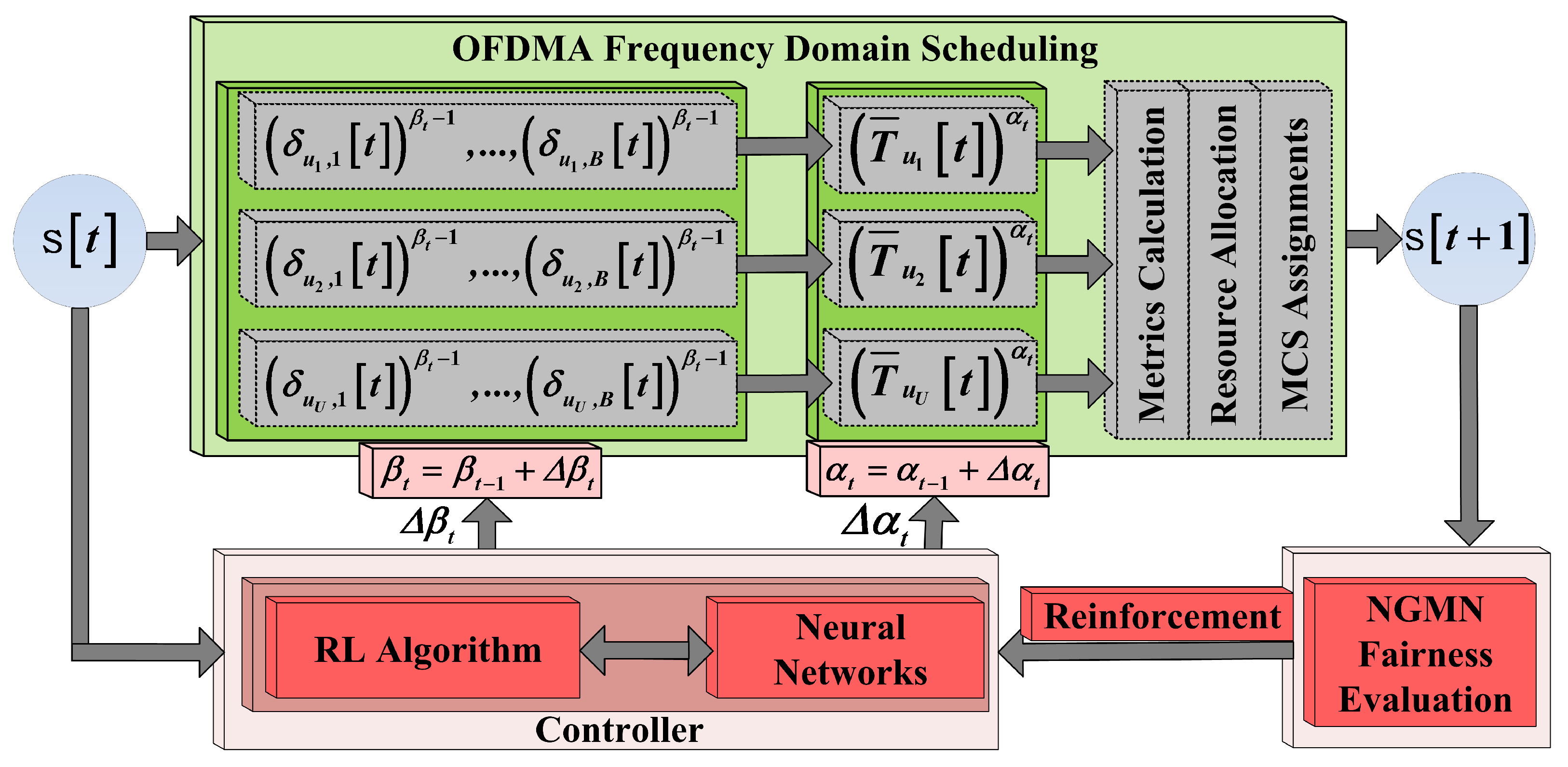
where { Δ α t , Δ β t } [ 1 , 1 ] are the fairness steps that need to be set in each TTI in order to meet the NGMN feasible region. When SP-GPF is optimized, only α t is adapted at each TTI since β = 1 for the entire transmission. As shown in Figure 2, the fairness steps are decided by an intelligent controller at each TTI. In general, the controller makes use of RL algorithm and neural network approximation to map the scheduler momentary state s S to proper parameterization steps [ Δ α t , Δ β t ] . The fairness parameters are adapted based on Equation (7), and the scheduling process is conducted by following the resource allocation problem: utility calculation, metrics calculation, resource allocation, and MCS assignment for each allocated user. In the next TTI t + 1 , the NGMN fairness evaluation is performed to reinforce the controller such that its decisions could be improved.

5. Learning Framework

The purpose of the learning framework is to solve the optimization problem from Equation (5) by selecting at each TTI the fairness steps that can maximize the time when the NGMN fairness requirement is respected. As seen in Figure 2, the controller works with the OFDMA scheduler in iterations. At each TTI, the controller observes a state and takes an action. In the next TTI, the performance of the action applied in the previous TTI is evaluated based on the NGMN fairness criterion. A reward value is computed in this sense as a result of matching the obtained CDF plot to the NGMN fairness requirements, Υ R and Υ M . This value is reinforced and the controller updates the neural networks in order to improve its decision-making. This process is repeated for a consistent time period until the given convergence criterion is met.

5.1. Scheduler-Controller Interaction

We define in this subsection the controller states, actions, and rewards for the scheduling optimization problem that aims at meeting the NGMN fairness requirement at each TTI.

5.1.1. States

We define the continuous and multidimensional scheduler state space as S . At each TTI t, the controller perceives a momentary state s [ t ] S divided in two sub-states s [ t ] = [ s c [ t ] , s u [ t ] ] , where (a) s c [ t ] S c is the controllable sub-state that evolves according to the applied action at each TTI and (b) s u [ t ] S u is the uncontrollable scheduler state which cannot be predicted. The controllable state is defined as: s c [ t ] = [ α t 1 , β t 1 , T ^ , d ] , where T ^ = [ T ^ u 1 , T ^ u 2 , , T ^ u U ] , and d is determined as follows: (a) if the scheduler is unfair, then d = m a x u ( d u ) , where u U t are those users with the percentiles located in the unfair region; (b) if the scheduler is fair, then the distance becomes d = m i n u ( d u ) , where u are those users with the normalized throughput of T ˜ u 1 + ζ . By using the state element d, the controller is aware of how far or close the scheduler is from the unfair region. The uncontrollable state is s u [ t ] = [ cqi , U t ] , where cqi = [ cqi u 1 , cqi u 2 , , cqi u U ] , representing the vector of CQI indicators that depends on U t and the number of RBs B. Since both vectors cqi and T ^ depend on the number of active users U t at each TTI t, the dimension of the scheduler state space is variable over time. Then, we use methods from References [4,33] to compress T ^ and cqi , respectively, and get a constant dimension of the scheduler state space. In the rest of the paper, we are referring to s [ t ] S as a compressed state at TTI t.

5.1.2. Actions

The controller action at TTI t is defined by a [ t ] = [ Δ α t , Δ β t ] A = { a 1 , a 2 , , a A } for DP-GPF and a [ t ] = [ Δ α t ] A when the parameterization of SP-GPF is considered. Most of the existing RL algorithms (i.e., Q-learning [12], ACLA [38]) work with discrete action space representation and the fairness steps [ Δ α t , Δ β t ] or Δ α t need to be fixed and a priori determined. In this case, we need a set of | A | neural networks, where each controller action a A is represented by one neural network. At each TTI, the action representing certain fairness steps that corresponds to the neural network with the highest output is selected to update [ α t , β t ] or α t and conduct the scheduling process. Some other RL algorithms (i.e., Continuous ACLA [4]) require a continuous action space A . In this case, only one neural network is used to take as input the momentary scheduler states s S and to provide the continuous fairness steps [ Δ α t , Δ β t ] or Δ α t as outputs.

5.1.3. Reward Functions

The reward value represents the expected goodness of applying action a [ t ] A in state s S [39]. For our purpose, the reward function is computed while being taken into account two aspects: (a) based on the difference d u of user percentiles, we determine if the system is unfair, feasible, or over-fair; (b) if the scheduler is over-fair or unfair, then the reward should monitor if the applied fairness steps in the previous state are appropriate options that can drive the system to the feasible regions in next states. We further consider s [ t + 1 ] = s S and the following notations: (a) s c UF if the scheduler is unfair; (b) s c FS when the scheduler is feasible at TTI t + 1 ; and finally, (c) s c OF when the scheduler is over-fair. The proposed reward function is defined as r : S × A R and calculated as follows:
r t + 1 ( s , a ) = r u ( s , a ) , if s c UF , 1 , if s c FS , r o ( s , a ) , if s c OF ,
where the state of controllable elements can be calculated by giving the scheduling transition function [33]: s c = f ( s , a ) . The reward functions { r u , r o } are calculated based on the chosen parameterization model. Let us define { r u s , r o s } as the reward functions for the unfair and over-fair regions, respectively, when the SP-GPF is considered. If the DP-GPF parameterization is preferred, then we define the corresponding rewards as { r u d , r o d } for the unfair and over-fair regions, respectively.
When the unfair region is reached, the applied actions should be able to drive the scheduler back to the feasible region. For the SP-GPF, this reward function can be computed as follows:
r u s ( s , a ) = Δ α t , if Δ α t > 0 , 1 , if Δ α t 0 .
which aims that, when α t α t 1 , the scheduler can move much deeper in the unfeasible region and the afferent action must be punished. For the DP-GPF parameterization, the reward computation is divided in two components: (a) as long as α t β t , parameter α t must be increased in order to get the feasible region; (b) as long as α t < β t , the scheduler aims to increase the system throughput in the detriment of JFI fairness and, consequently, the unfair region is kept. In this case, the reward function should be monitored particularly for each fairness parameter, as proposed bellow:
r u d ( s , a ) = Δ α t , if α t β t , Δ α t > 0 , Δ α t , if α t β t , Δ α t 0 , 1 , if α t < β t , Δ α t 0 , Δ β t 0 , 0.5 · ( 1 + | Δ β t | ) , if α t < β t , Δ α t 0 , Δ β t < 0 , 0.5 · ( | Δ α t | + 1 ) , if α t < β t , Δ α t > 0 , Δ β t 0 , 0.5 · ( | Δ α t | + | Δ β t | ) , if α t < β t , Δ α t > 0 , Δ β t < 0 .
When the scheduler reaches the over-fair state, the range of fairness parameters must be adapted accordingly in order to reduce the level of JFI fairness and to increase the overall system throughput. The proposed reward function for the SP-GPF scheduling rule is computed as follows:
r o s ( s , a ) = Δ α t , if Δ α t < 0 , 1 , if Δ α t 0 .
which aims that parameter α t must be decreased in order to get the state status of s c FS ; otherwise, the applied fairness steps in the previous state must be punished by setting r o s = 1 . For the double parameterization scheme, we define two cases: (a) when α t β t , it is more likely that the scheduler would be predisposed to reach over-fairness regions in the future and, then, the best practice would be to decrease α t and to increase β t ; (b) when α t < β t , the system can converge a little bit faster to the desired region by simply increasing the value of β t . The proposed reward function for DP-GPF scheduling rule when the state is s c OF becomes the following:
r o d ( s , a ) = 1 , if α t β t , Δ α t 0 , Δ β t 0 , 0.5 · ( 1 + | Δ β t | ) , if α t β t , Δ α t 0 , Δ β t > 0 , 0.5 · ( | Δ α t | + 1 ) , if α t β t , Δ α t < 0 , Δ β t 0 , 0.5 · ( | Δ α t | + | Δ β t | ) , if α t β t , Δ α t < 0 , Δ β t > 0 , Δ β t , if α t < β t , Δ β t > 0 , Δ β t , if α t < β t , Δ β t 0 .
At the end of the learning stage, all RL algorithms should be able to maximize the number of rewards ( r = 1 ) and to minimize the amount of punishment rewards when r < 0 .

5.2. Learning Functions

The RL framework aims to learn over time based on the tuple [ s , a , r , s ] the best functions able to map momentary scheduler states to fairness steps. Conceptually, these functions must be learnt based on some policies π ( a s ) , where π is the probability of selecting action a [ t ] = a in state s [ t ] = s being defined as follows [39]:
π ( a s ) = P a [ t ] = a | s [ t ] = s .
If we consider A = { a 1 , a 2 , , a A } as a discrete set of actions, then one of the most well-known learning functions that can be developed while following policy π is the action-value function Q π : S × A R defined under its original form as follows [39]:
Q π ( s , a ) s t a c k r e l ( def ) = E π t = 0 γ t R t + 1 | s [ 0 ] = s , a [ 0 ] = a ,
where (a) ( γ t R t + 1 ; t 0 ) is the accumulated reward value being averaged from state to state by the discount factor γ [ 0 , 1 ] ; (b) s [ 0 ] is considered as random such that P ( s [ 0 ] = s ) > 0 holds for every state s S ; and (c) P ( a [ 0 ] = a ) > 0 holds for all fairness steps a A . Once the learning stage is completed, in each state s S , we get a vector of action values [ Q ( s , a 1 ) , Q ( s , a 2 ) , , Q ( s , a | A | ) ] , where the action with the highest function value is selected to conduct the scheduling process. However, the actor-critic RL algorithms consider an additional state-value function V π : S R that is used to learn the value of the entire policy π on each state, defined as follows [39]:
V π ( s ) = ( def ) E π t = 0 γ t R t + 1 | s [ 0 ] = s .
The state-value function can be learnt to criticise the fairness decisions taken at each TTI based on Q ( s , a ) . The learning quality of actor-critic RL algorithms can be improved since the potentially good actions are encouraged to be selected based on the state-value function V π .
Both action-value and state-value functions must be updated at each TTI as a result of the interaction between the OFDMA scheduler and controller. To this extent, we deploy the transition functions corresponding to Equations (14) and (15) as follows [33]:
Q π ( s , a ) = r ( s , a ) + γ · Q π ( s , a ) ,
V π ( s ) = r ( s , a ) + γ · V π ( s ) ,
where s S is considered the actual state when the state-value and action-value functions can be updated as a result of applying action a A in momentary state s S . These functions are learnt for a consistent amount of TTIs until given the convergence criterion is respected.
The best practice is to obtain the optimal versions of state-value and action-value functions when the learning process is finished. We define V * : S R as an optimal state-value function that represents the highest expected return when the process is started from state s [ 0 ] S and V * ( s ) = m a x π V π ( s ) [39]. In a similar way, Q * : S × A R is the optimal action-value function and represents the highest expected return when the scheduling starts from s [ 0 ] S and the first applied fairness parameters correspond to action a [ 0 ] A . Once the optimality condition is met, at each TTI, we aim to select the action with the highest output as follows:
a * = a r g m a x a A [ π ( a s ) ] .
Consequently, the action-value function that follows the policy π ( a s ) becomes Q π ( s , a ) = m a x a A Q * ( s , a ) Then, Equations (16a) and (16b) can be rewritten as follows:
Q * ( s , a ) = r ( s , a ) + γ · m a x a A Q * ( s , a ) ,
V * ( s ) = r ( s , a ) + γ · V * ( s ) .
The optimal state-value function can be additionally determined as V * ( s ) = m a x a A Q * ( s , a ) . The transition between states for the optimal state-value and action-value functions can keep the same form as Equations (18a) and (18b), respectively, or alternatively, can be developed as shown bellow:
Q * ( s , a ) = r ( s , a ) + γ · V * ( s ) ,
V * ( s ) = r ( s , a ) + γ · m a x a A Q * ( s , a ) .
As already stated, the multidimensional representation of the scheduler state space makes the use of look-up tables for Q ( s , a ) and V ( s ) an impossible task since the state-action pairs cannot be enumerated exhaustively. Then, the optimal state-value and action-value functions can be only approximated. In this sense, we use feed forward neural networks as function approximations in order to learn the most appropriate fairness steps to be applied on each scheduler state.

5.3. Approximation of Learning Functions with Feed Forward Neural Networks

Let us define Q * ¯ : S × A [ 1 , 1 ] as the approximation of optimal action-value function, represented by the following nonlinear function:
Q * ¯ ( s , a ) = h a ( θ t a , ψ ( s ) ) ,
where [ h a 1 , h a 2 , , h a A ] are the feed forward neural networks used to approximate the action-value function for each action a A . Additionally, ψ is the feature vector consisting the nonlinear transformations of neural nodes and [ θ t a 1 , θ t a 2 , , θ t a A ] is the vector of weights that need to be updated at each TTI. Based on Equation (20a), the action space is discrete, each action a A has a separate neural network h a , and only one set of weights corresponding to θ t a is updated at TTI t if action a { a 1 , a 2 , , a A } is applied at TTI t 1 . If the action space is continuous, then we use only one neural network to approximate the best fairness steps to be applied on each momentary state s S . According to the developed parameterization scheme, the approximation of optimal action-value function is defined as follows: (a) for the SP-GPF optimization with the momentary action of a [ t ] = Δ α t , we define the approximated action-value function as Q * ¯ : S [ 1 , 1 ] ; (b) for the DP-GPF parameterization scheme with continuous a [ t ] = [ Δ α t , Δ β t ] , the approximated action-value function becomes Q * ¯ : S [ 1 , 1 ] 2 . Regardless of the type of parameterization, the nonlinear representation for the approximated action-value function can be written as follows:
Q * ¯ ( s ) = h q ( θ t q , ψ ( s ) ) ,
where h q is one action-value neural network for the continuous action space and θ t q is the set of weights trained to provide the most appropriated actions a [ t ] = Δ α t or a [ t ] = [ Δ α t , Δ β t ] on each state.
For actor-critic RL algorithms, the optimal state-value function can be approximated by defining the nonlinear function V * ¯ : S [ 1 , 1 ] represented by the following:
V * ¯ ( s ) = h v ( θ t v , ψ ( s ) ) ,
where h v is the state-value neural network and θ t v is the set of weights that are trained to give the value of certain policy. In general, both neural networks from Equations (20a) and (20c) are updated at each TTI when the actor-critic RL schemes are performed. However, some actor-critic algorithms may impose a critic condition to update only those neural networks corresponding to the potentially good actions.
To summarize, function Q * ¯ is an approximation of optimal action-value function Q * , while V * ¯ is the approximation of optimal state-value function V * . Feed forward neural networks are used to implement both functions Q * ¯ and V * ¯ . The idea is to update the weights of neural networks in the learning stage in order to get good suboptimal solutions of Q * and V * . One way to obtain such solutions is to monitor and minimize over the learning time the error between optimal values (given by the target functions from Equations (18a), (18b), (19a), and/or (19b)) and the actual response of neural networks given by Q * ¯ and V * ¯ , respectively. By failing to minimize these errors, the decisions of neural networks can be inadequate and, consequently, the applied fairness steps fail to localize over time the feasible fairness region. The calculation of these errors differs from one RL algorithm to another. Before detailing the types of RL algorithms used to perform the NGMN fairness optimization, the following subsections present the insights of propagating the errors through the neural networks.

5.4. Training the Feed Forward Neural Networks

The neural networks consist of processing nodes arranged in layers. If we consider a total number of L layers, then N l is the number of nodes of layer l { 1 , 2 , , L } . However, the best set of parameters in { L , N l } , l = 1 , 2 , , L must be a priori decided before launching the learning stage. Additionally, as indicated in Equation (20a–c), the neural networks make use of a weights vector { θ t a 1 , θ t a 2 , , θ t a A , θ t v } , or { θ t q , θ t v } that are used to interconnect the adjacent layers one by one. The number of weighs that must be tuned between layers l and l + 1 is ( N l + 1 ) × N l + 1 . For the entire neural network, there is a total number of l = 1 L 1 ( N l + 1 ) × N l + 1 weights that are updated each time.
The neural weights are updated at each TTI as a result of using certain fairness steps when performing the NGMN fairness based scheduling problem. We consider the actual state s S when the neural networks are updated based on the applied action a A in previous state s S . For a given neural network (i.e., h v , h q , or h a ), a target network value for the applied action a A in state s S is determined based on the reward value r ( s , a ) received in state s S . The weights are updated based on two processes: (1) forward propagation when the learnt network value is calculated by forwarding through the neural network the previous and current states { s , s } S ; (2) back propagation, where the error between the learnt and target values is back-propagated through the neural network and the weights are updated accordingly layer-by-layer.

5.4.1. Forward Propagation

Let us consider the matrix of weights W l = { w c , d , c = 1 , , N l , d = 1 , , N l + 1 } used to interconnect layers l and l + 1 . The general representation for the nonlinear approximation of optimal state-value function can be written as follows [40]:
V * ¯ ( s ) = ψ L ( W L 1 T · · ψ l + 1 ( W l T · · ψ 2 ( W 1 T · s ) ) ) ,
where ψ l = [ ψ l , 1 , ψ l , 2 , , ψ l , N l ] is the vector of activation functions used as nonlinear computations for each node within each layer. A similar representation is used for the action-value functions when the set of actions is discrete or continuous. In the case of RL algorithms with discrete action spaces, only the action-value neural network Q * ¯ ( s , a ) is updated as a result of applying action a A in state s S .
The set of weights { θ t v , θ t a } or { θ t v , θ t q } are updated based on the corresponding error values that are reinforced on each TTI. For the state-value function, we define the error function as e v : [ 1 , 1 ] 2 × | S | + 1 [ 1 , 1 ] , which is calculated as follows [40]:
e t + 1 v ( θ t v , s , s ) = V T ( s ) V * ¯ ( s ) ,
where V T ( s ) is the target state-value function that can be calculated following Equations (18b) or (19b). The forward propagation of the state-value neural network determines both values { V * ¯ ( s ) , V * ¯ ( s ) } needed to calculate the error from Equation (22a). When the action space is discrete, we define the error function for action a A as e a : [ 1 , 1 ] 2 × | S | + 1 [ 1 , 1 ] and the computation formula as presented bellow [40]:
e t + 1 a ( θ t a , s , s ) = Q T ( s , a ) Q * ¯ ( s , a ) ,
where the target action-value function Q T ( s , a ) is determined based on Equations (18a) or (19a). Basically, when the RL algorithms make use of discrete action spaces, only two neural networks are updated at each TTI such as { h v , h a } , where a A is applied in the previous state s S . For the case of continuous action space, the action-value error is defined as e q : [ 1 , 1 ] 2 × | S | + 1 [ 1 , 1 ] N , where N = 1 for SP-GPF and N = 2 for DP-GPF. This error is determined based on the following formula:
e t + 1 q ( θ t q , s , s ) = Q T ( s ) Q * ¯ ( s ) ,
where the target action-value Q T ( s ) is determined based on a given policy π of selecting the fairness steps in each scheduler state during the learning stage.

5.4.2. Backward Propagation

Once the momentary states { s , s } S are propagated and the errors are computed, the back-propagation procedure aims to calculate for each node the corresponding error and to update the neural weights from layer-to-layer. If we define for the state-value neural network the vector of errors e l v = [ e l , 1 v , e l , 2 v , , e l , N l v ] at the output of layer l { 1 , 2 , , L } , then these errors are determined by back-propagating from right to left all error vectors at the output of layer l. From layer l + 1 to layer l, the vector of errors is back-propagated by using the following equation [40]:
e l v = W l T × T ( Ψ l + 1 , e l + 1 v ) ,
where Ψ l + 1 = [ ψ l + 1 , 1 , ψ l + 1 , 2 , , ψ l + 1 , N l + 1 ] is the vector of derivative activation functions of layer l + 1 and T ( Ψ l + 1 , e l + 1 v ) = [ ψ l + 1 , 1 · e l + 1 , 1 v , ψ l + 1 , 2 · e l + 1 , 2 v , , ψ l + 1 , N l + 1 · e l + 1 , N l + 1 v ] . Once the errors are back-propagated from the output to the input layers by using Equation (23), the matrix of weights between each adjacent layers can be updated. Individually, the weight w c , d t + 1 that interconnects nodes c { 1 , 2 , , N l } and d { 1 , 2 , , N l + 1 } is updated as follows [40]:
w c , d t + 1 = w c , d t + η t + 1 · s l , c · ψ l + 1 , d · e l + 1 , d v ,
where η t + 1 is the learning rate at TTI t + 1 and s l , c is the value of the state element propagated to node c { 1 , 2 , , N l } of layer l { 1 , 2 , , L } . The error back-propagation for action-value neural networks follows the same reasoning with the amendment that, when the action space is continuous, the initial error e L q is two-dimensional for the DP-GPF parameterization scheme.

5.5. Exploration Types

At the beginning of the learning stage, the weights { θ v , θ a 1 , , θ a A } or { θ v , θ q } are randomly chosen in a certain interval. By only exploiting the neural networks to provide the fairness steps, some actions could be starved in getting explored properly and the learning performance could be very poor. Therefore, the learning policy may decide to ignore the neural networks for given time intervals and to select random actions to be applied in the scheduling process. When the action space is discrete, a random action that may not correspond to the neural network with the highest value can be selected to perform the scheduling procedure. When the action space is continuous, random fairness steps (different from those provided by the action-value neural network) can be used. This stage in the learning phase when random actions are selected instead of using the values provided by the neural networks is entitled improvement. On the other side, the evaluation steps aims to exploit what the neural networks have learnt so far. In the learning stage, the trade-off between improvements and evaluations is decided by certain distributions such as ϵ -greedy or Boltzmann [40]. When the action space is discrete, the ϵ -greedy policy selects the action a A to be applied on state s S based on the following probability [40]:
π ( a s ) = ϵ t ( a ) ϵ t ϵ , h a [ θ t a , ψ ( s ) ] ϵ t < ϵ ,
where ϵ t ( a ) is the random variable associated to action a A , ϵ [ 0 , 1 ] is a parameter that decides when the improvement or evaluation steps should take place and keeps the same value for all actions, and ϵ t [ 0 , 1 ] is random variable provided each TTI. When ϵ is low enough, more improvements are used to perform the fairness-based scheduling optimization problem. However, in both cases of improvement and evaluation steps, the action a * A to be performed is determined based on Equation (17). Following the same ϵ -greedy policy for RL framework with continuous actions spaces, the action selection is determined based on the following:
a [ t ] = ε t = [ ϵ t 1 , , ϵ t N ] ϵ t ϵ , Q * ¯ ( s ) = [ s L , 1 , , s L , N ] ϵ t < ϵ .
If ϵ is small, then an improvement step is performed and the action a takes a random real number in the range of ε t [ 1 , 1 ] N . Otherwise, the output of the neural network is exploited and a [ t ] = Q * ¯ ( s ) . It is worth mentioning that, when N = 1 , we consider the SP-GPF parameterization, whereas when N = 2 , the output of neural network is two-dimensional and s L , 1 = Δ α t and s L , 2 = Δ β t for DP-GPF scheduling rule.
The Boltzmann distribution can be used only for discrete action spaces, and it takes into account the response of neural networks in each momentary state. The actions with higher neural network values should have higher chances to be selected on the detriment of other actions with lower values. The potentially better fairness steps to be applied can be detected by following the formula [40]:
π ( a s ) = e x p [ h a ( θ t a , ψ ( s ) ) / τ ] a = a 1 a A e x p [ h a ( θ t a , ψ ( s ) ) / τ ] ,
where τ is a temperature factor that decides how greedy the action selection is. When τ is low, the neural network with the highest value is more likely to perform the scheduling procedure. When τ gets very high values, then the selection is more random and all policies { π ( a 1 s ) , π ( a 2 s ) , , π ( a A s ) } will have nearly the same probability to be selected.

5.6. RL Algorithms

In this subsection, we present a set of RL algorithms used to update the feed forward neural networks at each TTI. These algorithms are differentiated based on the calculation formulas that are used to compute the errors and target values for state-value and action-value functions.
Q-Learning [12]: applicable for discrete action space and considers only the action-value neural networks; the target action-value function Q T ( s , a ) is calculated based on Equation (18a) and the error to be back-propagated is calculated by using Equation (22b).
Double Q-Learning [41]: makes use of two sets of action-value neural networks (a total of 2 A neural networks): Q A * ¯ ( s , a ) , where a = { a 1 , a 2 , , a A } , and Q B * ¯ ( s , b ) , where b = { a 1 , a 2 , , a A } . The target action-value functions for these sets of neural networks are determined as follows:
Q A T ( s , a ) = r ( s , a ) + γ · Q B * ¯ ( s , a * ) ,
Q B T ( s , b ) = r ( s , a ) + γ · Q A * ¯ ( s , b * ) ,
where a * = a r g m a x a Q A * ¯ ( s , a ) and b * = a r g m a x b Q B * ¯ ( s , b ) . At each TTI, the policy of selecting the action to be performed follows the following reasoning:
π ( a s ) = ϵ t ( a ) ϵ t ϵ , Q A * ¯ ( s , a ) + Q B * ¯ ( s , a ) ] / 2 ϵ t < ϵ .
Then, one of Q A * ¯ or Q B * ¯ is randomly updated by reinforcing the error calculated with Equation (22b).
SARSA [42] is an on-policy RL algorithm dedicated for discrete action spaces that follows a given policy π ( s , a ) , and the target action-value functions are determined according to the action decided in the current state s S as follows:
Q T ( s , a ) = r ( s , a ) + γ · Q * ¯ ( s , a * ) ,
where a * A is determined based on Equation (17) and the error to be reinforced is similar to Q-learning algorithm and follows the expression of Equation (22b).
QV-Learning [43] is an actor-critic RL algorithm that works with discrete action spaces and updates both state-value and action-value neural networks. The target action-value and state-value functions are determined based on Equations (19a) and (18b), respectively. The errors to back-propagate each TTI follow the same form of Equations (22a) and (22b), respectively.
QV2-Learning [44] uses a discrete representation for the action space and keeps similar computation formulas as QV-learning for the target functions and action-value error. The difference is represented by the state-value error, which is determined as follows:
e t + 1 v ( θ t v , s , s ) = V T ( s ) Q * ¯ ( s , a ) .
QVMAX-Learning [44] considers the calculation of { e a , e v } , and Q T ( s , a ) similar to QV-learning (Equations (22a), (22b) and (19a), respectively) while the target state-value function is determined based on Equation (19b).
QVMAX2-Learning [44] considers the target action-value function Q T ( s , a ) similarly to QV-learning (Equation (19a)), the target state-value function V T ( s ) is computed similar to QVMAX (Equation (19b)), the action-value error e a is based on Equation (22b), and the state-value error e v is similar to QV2-learning (Equation (31)).
Actor-Critic Learning Automata (ACLA) [38] is an actor-critic algorithm that updates the action-value neural network based on the state-value or critic error. The target state-value function is determined based on Equation (18b) and the error for state-value function follows the equation from Equation (22a). If the critic error e t + 1 v 0 , then the action a A applied in state s S is a good option and the target action-value should be maximized. Otherwise, the probability of selecting a A applied in state s S must be decreased. Therefore, ACLA proposes the computation of target action-value function as follows:
Q T ( s , a ) = 1 , if e t + 1 v ( θ t v , s , s ) 0 , 1 , if e t + 1 v ( θ t v , s , s ) < 0 ,
where the action-value error is back-propagated by using the computation of Equation (22b).
Continuous ACLA (CACLA) [45] is a modified version of ACLA-learning used to deal with continuous action spaces. For the RL algorithms that make use of discrete action spaces, pre-established fairness steps are applied in each state where each configuration is characterized by a neural network approximation. Compared to these approaches, CACLA uses only one neural network for the optimal action-value approximation that provides the continuous fairness steps to parameterize SP-GPF or DP-GPF scheduling rules. Similar to ACLA algorithm, the target state-value function and the state-value error are calculated based on Equations (18b) and (22a), respectively. However, the target action-value function is Q T ( s ) = a [ t ] , where a [ t ] is determined based on Equation (26) and the error is back-propagated by using Equation (22c). We refer to CACLA-1 RL algorithm when we optimize the SP-GPF and the action-value neural network learns only Δ α t to be applied at each TTI t. CACLA-2 is used when the DP-GPF parameterization is considered, and a two-dimensional output is provided by the neural network to represent the temporal [ Δ α t , Δ β t ] fairness steps.

6. Simulation Results

Simulation results are obtained by using the RRM-Scheduler simulator [4], a C++ tool that inherits the Long Term Evolution Simulator (LTE-Sim) [35] by implementing additional functions such as advanced state-of-the-art OFDMA schedulers, RL algorithms used in different scheduling problems, neural network approximation for RL decisions, and CQI compression schemes. To evaluate the performance of the proposed framework under various RL algorithms, we use an infrastructure of 10 Intel(R) 4-Core(TM) machines with i7-2600 CPU at 3.40 GHz, 64 bits, 8 GB RAM, and 120 GB HDD Western Digital storage. In the first step, the framework runs the learning stage under different RL algorithms and various networking conditions to apply the most appropriate fairness steps on each state such that the NGMN fairness requirement is met. Then, the obtained nonlinear functions for each RL algorithm are compared based on NGMN evaluations that consider both EMF and MMF types of filters. Then, the performance of the most promising RL-based nonlinear functions is compared to the most relevant adaptive scheduling techniques from literature.

6.1. Parameter Settings

Both SP-GPF and DP-GPF scheduling rules are used when evaluating the NGMN fairness performance. For the SP-GPF parameterization with discrete action space, the following set of actions is considered: a [ t ] = Δ α t { ± 10 4 ; ± 10 3 ; ± 10 2 ; ± 5 · 10 2 ; ± 10 1 ; 0 } . The RL algorithms used to deal with this discrete action set are Q-Learning [12], DQ-Learning [41], SARSA [42], QV [43], QV2 [44], QVMAX [44], QVMAX2 [44], and ACLA [38]. The number of neural networks to be trained at each TTI by each of these RL algorithms is A = 11 . For the continuous action space of SP-GPF, CACLA-1 is used to learn the best approximation of Δ α t to be applied at each momentary state s S . For DP-GPF parameterization, a proper setting of the discrete action set is very difficult to be achieved due to the very high number of actions that would result from the combination of Δ α and Δ β steps. Therefore, CACLA-2 is used to perform the DP-GPF parameterization for the continuous action a [ t ] = [ Δ α t , Δ β t ] A only.
The learning stage is performed on all RL algorithms with the same networking conditions (i.e., channel conditions, number of active users, and same quota of data in the queues) for about 3000 s. Due to poor convergence properties to the given error threshold during this interval, we aim to extend the learning stage for Q-Learning, DQ-Learning, and SARSA algorithms with Experience Replay (ER) stage [46] for about 1000 s. For the first 3000 s, the RL controller is fully connected with the scheduler environment, while in the ER stage, the controller works in autonomous way. When connected with the scheduler environment, random samples from the unfair, over-fair, and feasible zones are stored by using the following format: ( s [ t ] = s , a [ t ] = a , r [ t + 1 ] = r , s [ t + 1 ] = s , a [ t + 1 ] = a ) . In the ER stage, the stored samples ( s , a , r , s , a ) are randomly revisited in order to improve the generalizations of feed forward neural networks only for the Q, DQ, and SARSA RL algorithms. In the exploitation stage, the learnt nonlinear functions for each RL algorithm are evaluated for 200 s while using the same networking conditions. We aim to evaluate the performance of these policies by monitoring the mean percentage of TTIs when (a) the scheduler is unfair: p ( s UF ) ; (b) the scheduler is feasible: p ( s FS ) ; and (c) the scheduler is over-fair: p ( s OF ) . We compare the proposed RL algorithms with the most relevant adaptive fairness-based schedulers from literature such as Maximizing Throughput (MT) [28] and Adaptive Scheduling (AS) [29].
The performance evaluation of NGMN fairness is conducted by using both types of filters when computing the average user rates. Studies regarding the setting of optimal forgetting factors ψ in OFDMA scheduling exist. The work conducted in Reference [47] denotes a small improvement in user throughput when setting values higher than ψ = 0.01 . When measuring NGMN performance, lower forgetting factors translate into significant oscillations in the obtained results, while higher values can limit seriously the contribution brought by the applied fairness steps in each state. Although the forgetting factor adaptation could represent an important future work to be addressed, in this paper, we set the value of this parameter to ψ = 0.01 . A very important parameter to set is the windowing factor ρ used to determine the average user rates with median moving filter. Setting optimal range of windowing factors is also crucial to other RL-based scheduling problems oriented on bit-rate or packet-loss requirements [33,34]. We aim at finding the optimal range of windowing factors able to provide the maximum number of TTIs when the scheduler is feasible by minimizing at the same time the amount of TTIs when the scheduler is declared unfair. Based on a priori simulations, we set the confidence factor to ζ = 0.05 . Below this limit, the controller is not able to localize the feasible region in the learning stage. Higher confidence intervals will involve a much fairer schedulers that can induce lower system throughput.

Network and Controller Settings

We consider a system bandwidth of 20 MHz where the total number of disposable resource blocks is equal to B = 100 . A cluster with 7 cells with the radius of 1 km is considered in our simulations, where the scheduling performance is evaluated in the central cell while other cells provide the interference levels. The number of users is varied in the range of U t = [ 15 , 120 ] during both learning and exploitation stages with the optimal number for maximum schedulable users U m a x = 10 . In the learning stage, the number of active users is randomly chosen in the range of 15 to 120 at each 1000 TTIs. Each user considers a full buffer traffic model and moves with 120 km/h speed using a random direction mobility model in both learning and exploitation stages in order to explore a high variety of CQI distributions. Frequency Division Duplex (FDD) is considered while the CQI reports are full-band and periodical. We are modeling the Radio Link Control (RLC) layer by using the Transmission Mode (TM) retransmission model since we are focused more on the performance of the applied fairness steps for the first transmission. The complete list of parameters for the network settings is presented in Table 1.
The controller parameterization aims to find the optimal settings in terms of exploration parameters ϵ or τ , discount factor γ , and learning rates { η V , η Q } for state-value and action-value neural networks, respectively. The aim would be the minimization of action-value and state-value errors for a given duration in the learning stage. Based on various tests conducted for a wide range of parameter configurations for each RL algorithm, Table 2 synthesizes the best parameterization scheme used for each RL algorithm.

6.2. Learning Stage

We run the learning stage for several configurations of neural networks in terms of the number of layers L and the number of hidden nodes for each layer N l , where l = 1 , 2 , , L . We keep the same configuration for action-value and state-value neural networks. The activation functions for the nodes of the input and output layers are linear. We consider tangent hyperbolic representation for the nodes belonging to the hidden layer. When higher configurations in terms of L and N l are used, the learnt nonlinear functions are more flexible in deciding the fairness steps to be applied in each TTI, the RL framework learns slower, and the system complexity is higher. When lower configurations are used in the learning stage, the nonlinear functions are less flexible, the RL framework can learn faster, and the system complexity is lower. Higher configurations of neural network may involve the over-fitting of input samples since the learnt nonlinear functions can represent very well the scheduler state space as well as other noisy data caused, for instance, by the random process of switching the number of active users at each 1000 TTIs. Lower configurations involve under-fitting since the learnt functions are inflexible and the overall state space is not very well generalized. According to the over-fitting/under-fitting trade-off for a learning period of 3000s, the configuration of ( L = 3 , N 2 = 60 ) provides constant time-based errors for all RL algorithms.

6.3. Exploitation Stage

In the exploitation stage, we run the learnt nonlinear action-value functions in parallel by using the same networking conditions for each RL algorithm. In total, 10 simulations are performed and the mean and standard deviations are evaluated when monitoring the fraction of the time (in subframes or TTIs) when the scheduler is unfair, feasible, and over-fair.
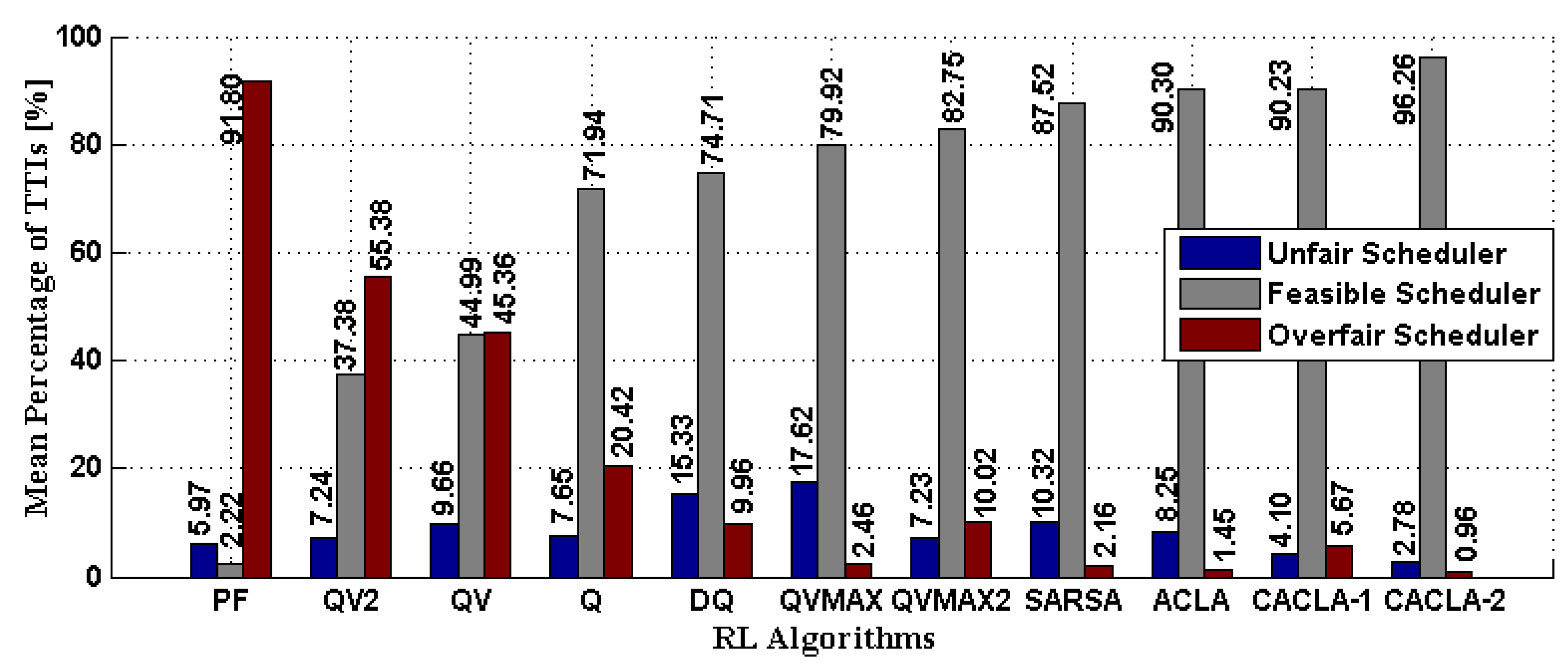
Figure 3 compares the RL algorithms when the EMF-based average user rates are used to evaluate the NGMN fairness requirement in terms of mean percentage of TTIs when the scheduler is unfair p ( s UF ) , feasible p ( s FS ) , and over-fair p ( s OF ) . The static PF scheduling rule ( α = 1 , β = 1 ) is over-fair for almost the entire scheduling session. The QV and QV2 algorithms aim to ensure acceptable p ( s UF ) but provide higher amounts of p ( s OF ) in the detriment of minimizing the time with feasible states. Q-learning, DQ-learning, and QVMAX decrease the percentage of TTIs with over-fair states, but unfortunately, the percentage of TTIs with unfair states is higher. QVMAX2 minimizes the drawbacks of previously mentioned RL schemes and improves the scheduling time when the scheduler is feasible. SARSA and ACLA aim to provide a minimum percentage of TTIs when the scheduler is over-fair, but a part of this gain is quantified on p ( s UF ) . However, CACLA-1 and CACLA-2 provide the best performance by maximizing p ( s FS ) and by minimizing at the same time p ( s UF ) and p ( s OF ) . The trained nonlinear functions with the following RL algorithms are the best top five options in terms of p ( s UF ) : CACLA-2, CACLA-1, ACLA, QVMAX2, and QV2. Figure 4 and Figure 5 present in more details the performances of CACLA-2, CACLA-1, QV2, and PF scheduling schemes when considering the state elements (d and [ α t , β t ] ) and the quantitative/qualitative evaluations.
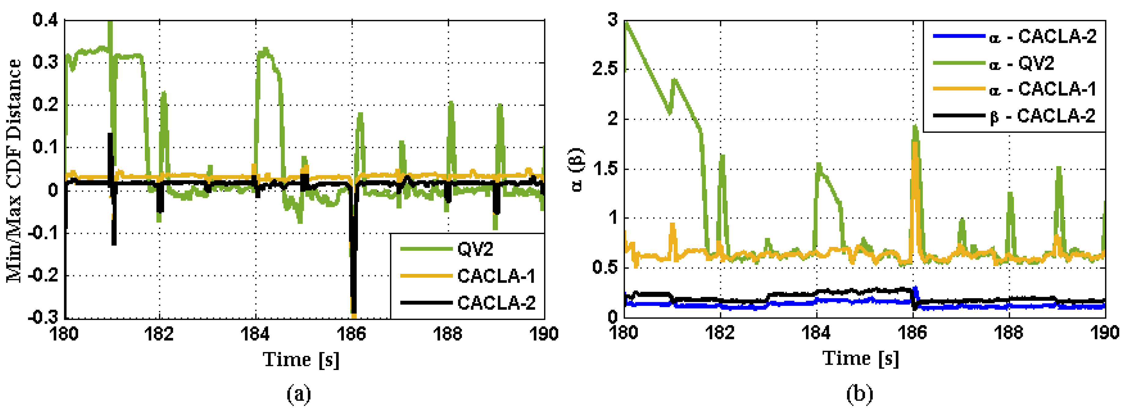
Figure 4a presents a time sequence in the exploitation stage for distance d between the NGMN fairness requirement and user throughput percentiles for the CACLA-2, CACLA-1, and QV2 algorithms. QV2 shows much higher distances in the over-fair region of the CDF plot when compared to CACLA-1 and CACLA-2. The same time sequence for the fairness parameters is presented in Figure 4b. When compared to CACLA-1, QV2 denotes higher α t values, placing it as the most over-fair option. However, by adapting both fairness parameters ( α t , β t ) , CACLA-2 is able to converge much faster to the feasible zone when compared to SP-GPF scheduling rule parameterized by CACLA-1.
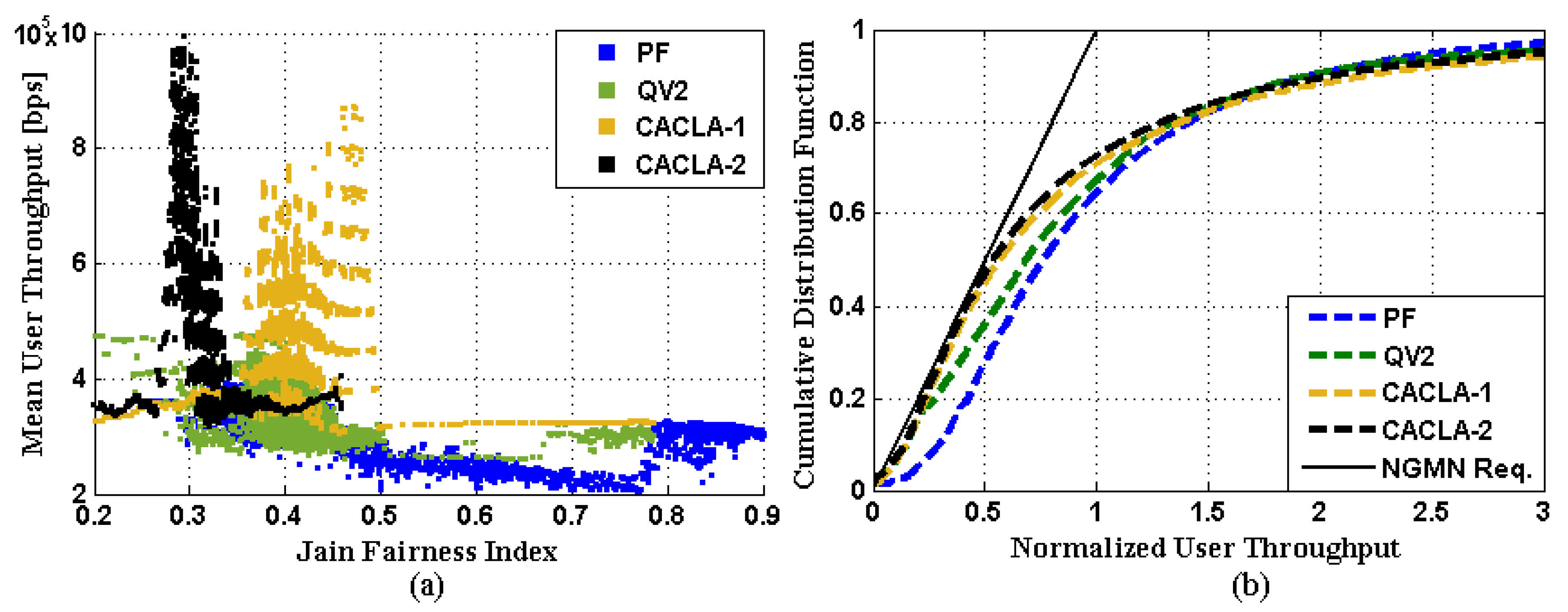
In Figure 5, we present the quantitative and qualitative evaluation for the same time sequence presented in Figure 4, The qualitative plot depicted in Figure 5b indicates that both CACLA-1 and CACLA-2 are feasible options while QV2 and PF scheduling schemes locate the CDF plot in the over-fair region. The quantitative evaluation in Figure 5a shows that CACLA-2 increases the system throughput when compared to CACLA-1 while still maintaining the feasible solution of NGMN fairness. This is expected since CACLA-2 provides lower d when reported to NGMN requirement as shown in Figure 4a. QV2 and PF scheduling schemes spread the quantitative trade-off points for a wide range of JFI values, placing them as over-fair solutions.
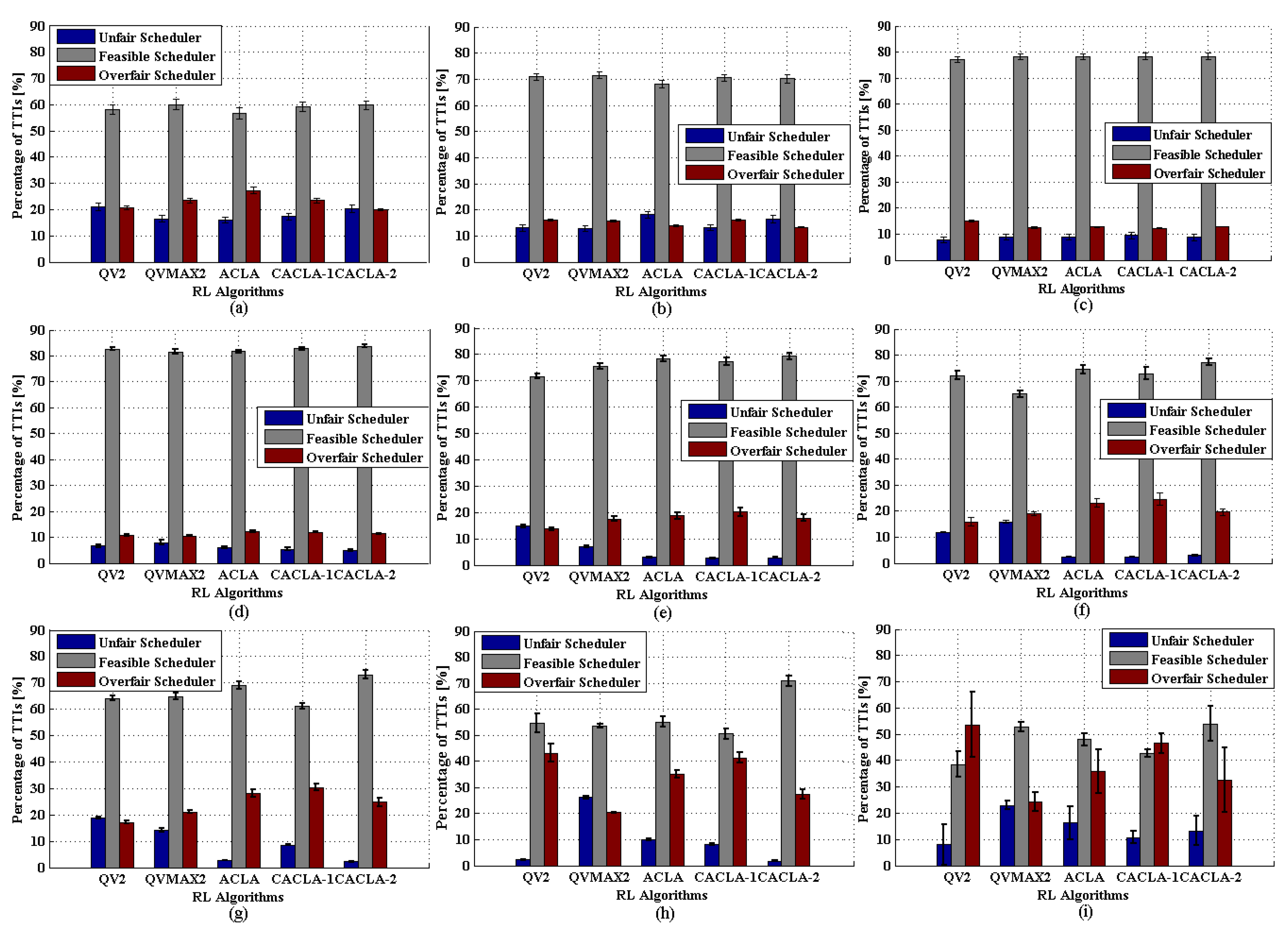
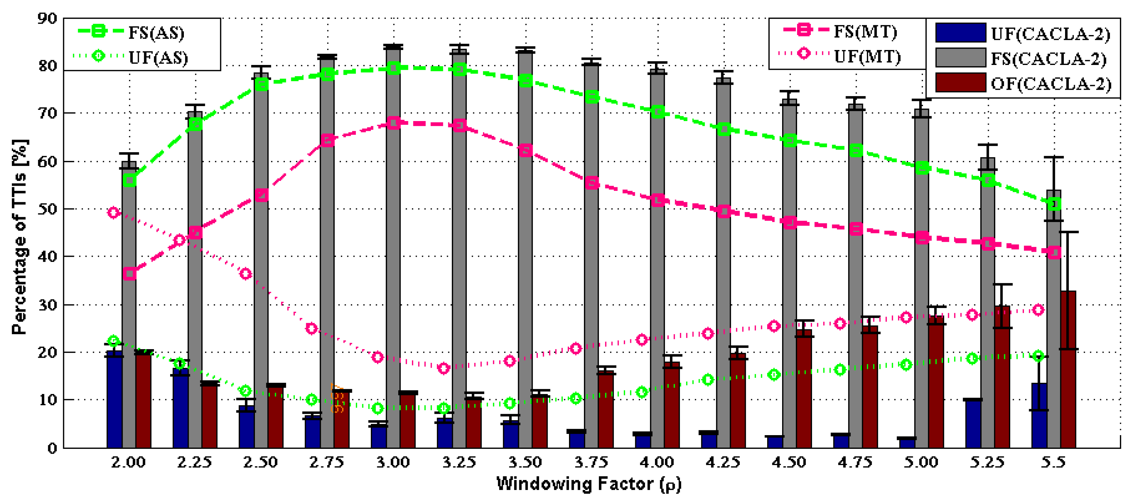
A comparison of the top five RL algorithms for different settings of windowing factor ρ is provided in Figure 6, where the average user throughput with the median moving filter is used to evaluate if the NGMN fairness requirement is achieved. When the windowing factor takes low values such as ρ = 2.0 (Figure 6a), ACLA and QVMAX2 obtain the lowest p ( s UF ) and all RL algorithms provide nearly the same performance when the mean percentage of TTIs with feasible zones is measured ( p ( s FS ) 55 % ). By using the windowing factors in the range of ρ { 2.25 , 2.5 , 3.0 } (Figure 6b–d, respectively), the considered RL algorithms provide nearly the same performance by increasing gradually the amount of feasible TTIs from p ( s FS ) 70 % to p ( s FS ) 80 % as indicated in Figure 6b,d. When increasing the windowing factor to ρ = 4.0 (Figure 6e), ACLA, CACLA-1, and CACLA-2 are the best options by indicating the lowest percentage of TTIs when the scheduler is unfair. In this case, QV2 achieves an amount of p ( s FS ) lower with about 10 % when compared with CACLA-2. In Figure 6f, ACLA, CACLA-1, and CACLA-2 are still the best options when ρ = 4.25 but a much lower p ( s UF ) when compared to QV2 or QVMAX2 is provided. However, when ρ = 4.5 (Figure 6g), CACLA-2 and ACLA provide the best results when measuring p ( s UF ) and p ( s FS ) while the mean percentage of TTIs with over-fair states is larger with about 10% when compared to the performance obtained for ρ = 4.25 . By increasing the windowing factor to ρ = 5.0 (Figure 6h), CACLA-2 becomes the best choice by minimizing the amount of TTIs with unfair states and by increasing the percentage of feasible TTIs with more than 15% when compared to other RL candidates. As seen from Figure 6i ( ρ = 5.5 ), there is a consistent increase in the STandard Deviation (STD) values for the obtained results, meaning that the proposed RL algorithms are not able to provide high accuracy when approximating the best fairness steps to be applied in each state. CACLA-2 still provides the highest amount of p ( s FS ) , but the mean percentage of unfair TTIs is higher than that of QV2 or CACLA-1. Based on Figure 6, the following conclusions can be drawn: (a) for low windowing factors (i.e., ρ [ 2.0 , 3.0 ] ), QV2, QVMAX2, ACLA, CACLA-1, and CACLA-2 present similar performance; (b) when the windowing factor is ρ ( 3.0 , 4.25 ] , ACLA, CACLA-1, and CACLA-2 ensure a minimum p ( s UF ) and are, thus, the best options; and (c) for higher windowing factors of ρ > 4.25 , CACLA-2 remains the most feasible solution.
Figure 7 shows the performance comparison of CACLA-2 and state-of-the-art fairness adaptive schedulers MT and AS when the windowing factor is in the range of ρ [ 2.0 , 5.5 ] . For this range, CACLA-2 outperforms AS and MT in terms of p ( s UF ) and p ( s FS ) . In particular, for lower windowing factors such as ρ [ 2.0 , 3.0 ] , CACLA-2 provides a slightly better performance than AS. When compared to MT adaptive scheme, maximum gains higher than 50% are obtained when measuring p ( s FS ) and higher than 60% when computing p ( s UF ) (when ρ = 2.0 ). For medium values of ρ [ 3.25 , 4.25 ] , the gains of CACLA-2 are constantly increasing to more than 11% of p ( s UF ) and to more than 14% of p ( s FS ) when matched against the AS algorithm. When compared to MT for ρ = 4.25 , gains higher than 25% are obtained when monitoring p ( s UF ) , while the gains corresponding to p ( s FS ) keep similar values when compared to other cases of lower windowing factors. These gains become higher when the windowing factor belongs to ρ { 4.5 , 5.0 , 5.25 } . However, when ρ 5.25 , CACLA-2 still gets a higher percentage of feasible TTIs but the amount of TTIs with unfair states is increasing when compared to the cases of lower windowing factors. Also, we observe higher oscillations of p ( s FS ) and p ( s UF ) when ρ 5.25 since the impact of the fairness steps applied at each TTI cannot be sensed immediately when matching the CDF plot to NGMN fairness requirement.

6.4. General Remarks

When training the feed forward neural networks with different RL algorithms to approximate in each momentary state the best parameterization decision for SP-GPF or DP-GPF scheduling rules, the following aspects must be considered: (a) the training data-set; (b) the compression of scheduler state space; (c) the set-up of RL controller and neural network configuration; and (d) learning termination condition. When solving the NGMN fairness based optimization problems with reinforcement learning, the learning stage should be conducted through different regions of the scheduler state space (unfair, feasible, and over-fair) in order to avoid the local-optima problems involved when updating the weights of neural networks. Also, an additional dataset collected from the learning stage is needed to conduct the ER stage for some RL algorithms such as Q-learning, DQ-learning, or SARSA. The scheduler state space must be compressed in order to make the learning concept possible and to reduce the complexity for the entire framework. Based on a priori simulations, a proper parameterization of RL controller needs to be decided in order to reduce the learning time and to improve its quality. Time-based adaptation of exploration parameters ( ϵ , τ ) is also possible by finding the most suitable functions that can ensure the best learning performance and convergence. Multiple configurations of neural networks must be a priori tested in order to get the best generalization of the input state space as a result of the trade-off between over-fitting, under-fitting, and framework complexity. The termination condition for the learning stage should monitor the evolution of the state-value and action-value errors for a consistent number of iterations.

7. Conclusions

This paper proposes a reinforcement learning framework able to adapt the generalized proportional scheduling rule in each state with the purpose of improving the fraction of scheduling time (in TTIs) when the qualitative NGMN fairness requirement is met. We use feed forward neural networks as nonlinear functions to approximate the best fairness parameters for the generalized proportional fair scheduling rule to be applied at each TTI. Various reinforcement learning algorithms are implemented to learn the best nonlinear functions that can ensure the highest outcome in terms of NGMN fairness requirement. The purpose is to select the best RL algorithms that can provide the highest outcome from the perspective of meeting the NGMN fairness criterion under various network settings and circumstances.
The reinforcement learning algorithms employed in this paper can be divided based on the type of action space and parameterization scheme. Some reinforcement learning algorithms (Q-learning, Double-Q-Learning, SARSA, QV, QV2, QVMAX, QVMAX2, and ACLA) make use of discrete and finite action space by using some fixed and a priori determined fairness steps to parameterize the generalized proportional fair in each state. CACLA algorithm considers a continuous and infinite action space, and the adaptation of generalized proportional fair is achieved with continuous fairness steps. We develop and compare two types of parameterization schemes for generalized proportional fair, such as simple and double parameterization. For the simple parameterization, the Q-learning, Double-Q-Learning, SARSA, QV, QV2, QVMAX, QVMAX2, ACLA, and CACLA-1 algorithms are used separately to train the neural networks in order to determine the best parameter α t to be applied at each TTI. When the double parameterization scheme is used, the CACLA-2 algorithm is employed to learn both fairness steps ( α t , β t ) in each state. On one side, the algorithms with continuous action space can get a better generalization for the learnt neural networks due to higher flexibility when selecting the fairness steps. On the other side, the double parameterization scheme can converge faster to the fairness feasible region when compared to other simple parameterization algorithms.
The NGMN fairness criterion is measured at each TTI based on average user rates. The performance of each reinforcement learning algorithm is analyzed by using two types of averaging filters for the user throughput: exponential and median. When the exponential moving filter is used, the QV2, QVMAX2, ACLA, CACLA-1, and CACLA-2 algorithms work better while minimizing the time when the scheduler is declared unfair. When the median moving filter is employed, two main conclusions can be drawn: (a) for lower window size, the obtained sets of neural networks learnt with different RL algorithms provide comparable performance; (b) for larger window size, the feed forward neural network learnt with CACLA-2 algorithm shows better performance in terms of average time when the scheduler is feasible. When compared to adaptive schedulers from literature, CACLA-2 outperforms all candidates for the entire range of windowing factors.

Author Contributions

Conceptualization, I.-S.C., S.Z. and M.A.; Data curation, I.-S.C. and R.T.; Formal analysis, I.-S.C. and R.T.; Funding acquisition, P.K. and G.G.; Investigation, I.-S.C., P.K., R.T. and G.G.; Methodology, I.-S.C., M.A., R.T. and G.G.; Project administration, S.Z., M.A., P.K. and G.G.; Resources, P.K. and R.T.; Software, I.-S.C. and P.K.; Supervision, S.Z., M.A., P.K. and G.G.; Validation, I.-S.C., S.Z., M.A., P.K. and R.T.; Visualization, I.-S.C., M.A. and R.T.; Writing—original draft, I.-S.C.; Writing—review & editing, S.Z., M.A., P.K., R.T. and G.G.

Funding

This research was funded by the European Union Horizon 2020 Research and Innovation Programme for the NEWTON project Grant Agreement number 688503.

Conflicts of Interest

The authors declare no conflict of interest.

References

  1. Andrews, J.G.; Buzzi, S.; Choi, W.; Hanly, S.V.; Lozano, A.; Soong, A.C.K.; Zhang, J.C. What Will 5G Be? IEEE J. Sel. Areas Commun. 2014, 3, 1065–1082. [Google Scholar] [CrossRef]
  2. Calabrese, F.D.; Wang, L.; Ghadimi, E.; Peters, G.; Hanzo, L.; Soldati, P. Learning Radio Resource Management in RANs: Framework, Opportunities, and Challenges. IEEE Commun. Mag. 2018, 56, 138–145. [Google Scholar] [CrossRef]
  3. Comsa, I.-S.; Trestian, R. Information Science Reference. In Next-Generation Wireless Networks Meet Advanced Machine Learning Applications; Comsa, I.-S., Trestian, R., Eds.; IGI Global: Hershey, PA, USA, 2019. [Google Scholar]
  4. Comsa, I.-S. Sustainable Scheduling Policies for Radio Access Networks Based on LTE Technology. Ph.D. Thesis, University of Bedfordshire, Luton, UK, November 2014. [Google Scholar]
  5. Comsa, I.-S.; Zhang, S.; Aydin, M.; Kuonen, P.; Trestian, R.; Ghinea, G. Enhancing User Fairness in OFDMA Radio Access Networks Through Machine Learning. In Proceedings of the 2019 Wireless Days (WD), Manchester, UK, 24–26 June 2019; pp. 1–8. [Google Scholar]
  6. Capozzi, F.; Piro, G.; Grieco, L.A.; Boggia, G.; Camarda, P. Downlink Packet Scheduling in LTE Cellular Networks: Key Design Issues and a Survey. IEEE Commun. Surv. Tutor. 2013, 15, 678–700. [Google Scholar] [CrossRef]
  7. Comsa, I.-S.; Zhang, S.; Aydin, M.; Chen, J.; Kuonen, P.; Wagen, J.-F. Adaptive Proportional Fair Parameterization Based LTE Scheduling Using Continuous Actor-Critic Reinforcement Learning. In Proceedings of the IEEE Global Communications Conference (GLOBECOM), Austin, TX, USA, 8–12 December 2014; pp. 4387–4393. [Google Scholar]
  8. Comsa, I.-S.; Aydin, M.; Zhang, S.; Kuonen, P.; Wagen, J.-F.; Lu, Y. Scheduling Policies Based on Dynamic Throughput and Fairness Tradeoff Control in LTE-A Networks. In Proceedings of the IEEE Local Computer Networks (LCN), Edmonton, AB, Canada, 8–11 September 2014; pp. 418–421. [Google Scholar]
  9. Shi, H.; Prasad, R.V.; Onur, E.; Niemegeers, I. Fairness in Wireless Networks: Issues, Measures and Challenges. IEEE Commun. Surv. Tutor. 2014, 16, 5–24. [Google Scholar]
  10. Jain, R.; Chiu, D.; Hawe, W. A Quantitative Measure of Fairness and Discrimination for Resource Allocation in Shared Computer Systems; Technical Report TR-301; Eastern Research Laboratory, Digital Equipment Corporation: Hudson, MA, USA, 1984; pp. 1–38. [Google Scholar]
  11. Next Generation of Mobile Networks (NGMN). NGMN Radio Access Performance Evaluation Methodology. In A White Paper by the NGMN Alliance. 2008, pp. 1–37. Available online: https://www.ngmn.org/wp-content/uploads/NGMN_Radio_Access_Performance_Evaluation_Methodology.pdf (accessed on 12 October 2019).
  12. Sutton, R.S.; Barto, A.G. Reinforcement Learning: An Introduction; MIT Press Cambridge: Cambridge, MA, USA, 2018. [Google Scholar]
  13. Iacoboaiea, O.C.; Sayrac, B.; Jemaa, S.B.; Bianchi, P. SON Coordination in Heterogeneous Networks: A Reinforcement Learning Framework. IEEE Trans. Wirel. Commun. 2016, 15, 5835–5847. [Google Scholar] [CrossRef]
  14. Simsek, M.; Bennis, M.; Guvenc, I. Learning based Frequency and Time-Domain Inter-Cell Interference Coordination in HetNets. IEEE Trans. Veh. Technol. 2015, 64, 4589–4602. [Google Scholar] [CrossRef]
  15. De Domenico, A.; Ktenas, D. Reinforcement Learning for Interference-Aware Cell DTX in Heterogeneous Networks. In Proceedings of the IEEE Wireless Communications and Networking Conference (WCNC), Barcelona, Spain, 15–18 April 2018; pp. 1–6. [Google Scholar]
  16. Zhang, L.; Tan, J.; Liang, Y.-C.; Feng, G.; Niyato, D. Deep Reinforcement Learning-Based Modulation and Coding Scheme Selection in Cognitive Heterogeneous Networks. IEEE Trans. Wirel. Commun. 2019, 18, 3281–3294. [Google Scholar] [CrossRef] [Green Version]
  17. Naparstek, O.; Cohen, K. Deep Multi-User Reinforcement Learning for Distributed Dynamic Spectrum Access. IEEE Trans. Wirel. Commun. 2019, 18, 310–323. [Google Scholar] [CrossRef]
  18. Comsa, I.-S.; Aydin, M.; Zhang, S.; Kuonen, P.; Wagen, J.-F. Reinforcement Learning Based Radio Resource Scheduling in LTE-Advanced. In Proceedings of the International Conference on Automation and Computing, Huddersfield, UK, 10–10 September 2011; pp. 219–224. [Google Scholar]
  19. Comsa, I.-S.; Aydin, M.; Zhang, S.; Kuonen, P.; Wagen, J.-F. Multi Objective Resource Scheduling in LTE Networks Using Reinforcement Learning. Int. J. Distrib. Syst. Technol. 2012, 3, 39–57. [Google Scholar] [CrossRef]
  20. Comsa, I.-S.; De-Domenico, A.; Ktenas, D. Method for Allocating Transmission Resources Using Reinforcement Learning. U.S. Patent Application No. US 2019/0124667 A1, 25 April 2019. [Google Scholar]
  21. He, J.; Tang, Z.; Tang, Z.; Chen, H.-H.; Ling, C. Design and Optimization of Scheduling and Non-Orthogonal Multiple Access Algorithms with Imperfect Channel State Information. IEEE Trans. Veh. Technol. 2018, 67, 10800–10814. [Google Scholar] [CrossRef]
  22. Shahsavari, S.; Shirani, F.; Erkip, E. A General Framework for Temporal Fair User Scheduling in NOMA Systems. IEEE J. Sel. Top. Signal Process. 2019, 13, 408–422. [Google Scholar] [CrossRef]
  23. Kaneko, M.; Yamaura, H.; Kajita, Y.; Hayashi, K.; Sakai, H. Fairness-Aware Non-Orthogonal Multi-User Access with Discrete Hierarchical Modulation for 5G Cellular Relay Networks. IEEE Access 2015, 3, 2922–2938. [Google Scholar] [CrossRef]
  24. Ahmed, F.; Dowhuszko, A.A.; Tirkkonen, O. Self-Organizing Algorithms for Interference Coordination in Small Cell Networks. IEEE Trans. Veh. Technol. 2017, 66, 8333–8346. [Google Scholar] [CrossRef]
  25. Zabini, F.; Bazzi, A.; Masini, B.M.; Verdone, R. Optimal Performance Versus Fairness Tradeoff for Resource Allocation in Wireless Systems. IEEE Trans. Wirel. Commun. 2017, 16, 2587–2600. [Google Scholar] [CrossRef]
  26. Ferdosian, N.; Othman, M.; Mohd Ali, B.; Lun, K.Y. Fair-QoS Broker Algorithm for Overload-State Downlink Resource Scheduling in LTE Networks. IEEE Syst. J. 2018, 12, 3238–3249. [Google Scholar] [CrossRef]
  27. Trestian, R.; Comsa, I.S.; Tuysuz, M.F. Seamless Multimedia Delivery Within a Heterogeneous Wireless Networks Environment: Are We There Yet? IEEE Commun. Surv. Tutor. 2018, 20, 945–977. [Google Scholar] [CrossRef]
  28. Schwarz, S.; Mehlfuhrer, C.; Rupp, M. Throughput Maximizing Multiuser Scheduling with Adjustable Fairness. In Proceedings of the IEEE International Conference on Communications (ICC), Kyoto, Japan, 5–9 June 2011; pp. 1–5. [Google Scholar]
  29. Proebster, M.; Mueller, C.M.; Bakker, H. Adaptive Fairness Control for a Proportional Fair LTE Scheduler. In Proceedings of the IEEE International Symposium on Personal, Indoor and Mobile Radio Communications (PIMRC), Instanbul, Turkey, 26–30 September 2010; pp. 1504–1509. [Google Scholar]
  30. Comsa, I.-S.; Aydin, M.; Zhang, S.; Kuonen, P.; Wagen, J.-F. A Novel Dynamic Q-learning-based Scheduler Technique for LTE-advanced Technologies Using Neural Networks. In Proceedings of the IEEE Local Computer Networks (LCN), Clearwater, FL, USA, 22–25 October 2012; pp. 332–335. [Google Scholar]
  31. Comsa, I.-S.; De-Domenico, A.; Ktenas, D. QoS-Driven Scheduling in 5G Radio Access Networks—A Reinforcement Learning Approach. In Proceedings of the IEEE Global Communications Conference (GLOBECOM), Singapore, 4–8 December 2017; pp. 1–7. [Google Scholar]
  32. Comsa, I.-S.; Trestian, R.; Ghinea, G. 360 Mulsemedia Experience over Next Generation Wireless Networks—A Reinforcement Learning Approach. In Proceedings of the Tenth International Conference on Quality of Multimedia Experience (QoMEX), Cagliari, Italy, 29 May–1 June 2018; pp. 1–6. [Google Scholar]
  33. Comsa, I.-S.; Zhang, S.; Aydin, M.; Kuonen, P.; Yao, L.; Trestian, R.; Ghinea, G. Towards 5G: A Reinforcement Learning-based Scheduling Solution for Data Traffic Management. IEEE Trans. Net. Serv. Manag. 2018, 15, 1661–1675. [Google Scholar] [CrossRef]
  34. Comsa, I.-S.; Zhang, S.; Aydin, M.E.; Kuonen, P.; Trestian, R.; Ghinea, G. Guaranteeing User Rates with Reinforcement Learning in 5G Radio Access Networks. In Next-Generation Wireless Networks Meet Advanced Machine Learning Applications; Comsa, I.S., Trestian, R., Eds.; IGI Global: Hershey, PA, USA, 2019; pp. 163–198. [Google Scholar]
  35. Piro, G.; Grieco, L.A.; Boggia, G.; Capozzi, F.; Camarda, P. Simulating LTE cellular systems: An Open-Source Framework. IEEE Trans. Veh. Technol. 2011, 60, 498–513. [Google Scholar] [CrossRef]
  36. Song, G.; Li, Y. Utility-based Resource Allocation and Scheduling in OFDM-based Wireless Broadband Networks. IEEE Commun. Mag. 2005, 43, 127–134. [Google Scholar] [CrossRef]
  37. Comsa, I.-S.; Zhang, S.; Aydin, M.E.; Kuonen, P.; Trestian, R.; Ghinea, G. Machine Learning in Radio Resource Scheduling. In Next-Generation Wireless Networks Meet Advanced Machine Learning Applications; Comsa, I.S., Trestian, R., Eds.; IGI Global: Hershey, PA, USA, 2019; pp. 24–56. [Google Scholar] [Green Version]
  38. Wiering, M.A.; van Hasselt, H.; Pietersma, A.-D.; Schomaker, L. Reinforcement Learning Algorithms for Solving classification Problems. In Proceedings of the IEEE Symposium on Adaptive Dynamic Programming and Reinforcement Learning, Paris, France, 11–15 April 2011; pp. 1–6. [Google Scholar]
  39. Szepesvari, C. Algorithms for Reinforcement Learning: Synthesis Lectures on Artificial Intelligence and Machine Learning; Morgan: San Rafael, CA, USA, 2010. [Google Scholar]
  40. Van Hasselt, H.P. Insights in Reinforcement Learning Formal Analysis and Empirical Evaluation of Temporal- Difference Learning Algorithms. Ph.D. Thesis, University of Utrecht, Utrecht, The Netherlands, 2011. [Google Scholar]
  41. van Hasselt, H. Double Q-learning. Adv. Neural. Inf. Process. Syst. 2011, 23, 2613–2622. [Google Scholar]
  42. Rummery, G.A.; Niranjan, M. Online Q-Learning Using Connectionist Systems; Technical Note; University of Cambridge: Cambridge, UK, 1994. [Google Scholar]
  43. Wiering, M. QV(lambda)-Learning: A new On-Policy Reinforcement Learning Algorithm. In Proceedings of the 7th European Workshop on Reinforcement Learning, Utrecht, The Netherlands, 20–21 October 2005; pp. 17–18. [Google Scholar]
  44. Wiering, M.A.; van Hasselt, H. The QV Family Compared to Other Reinforcement Learning Algorithms. In Proceedings of the IEEE Symposium on Adaptive Dynamic Programming and Reinforcement Learning, Nashville, TN, USA, 30 March–2 April 2009; pp. 101–108. [Google Scholar]
  45. van Hasselt, H.; Wiering, M.A. Using Continuous Action Spaces to Solve Discrete Problems. In Proceedings of the International Joint Conference on Neural Networks, Atlanta, GA, USA, 14–19 June 2009; pp. 1149–1156. [Google Scholar]
  46. Adam, S.; Busoniu, L.; Babuska, R. Experience Replay for Real-Time Reinforcement Learning Control. IEEE Trans. Syst. Man Cybern. Part C 2012, 42, 201–212. [Google Scholar] [CrossRef]
  47. Proebster, M.C. Size-Based Scheduling to Improve the User Experience in Cellular Networks. Ph.D. Thesis, Universität Stuttgart, Stuart, Germany, 2016. [Google Scholar]
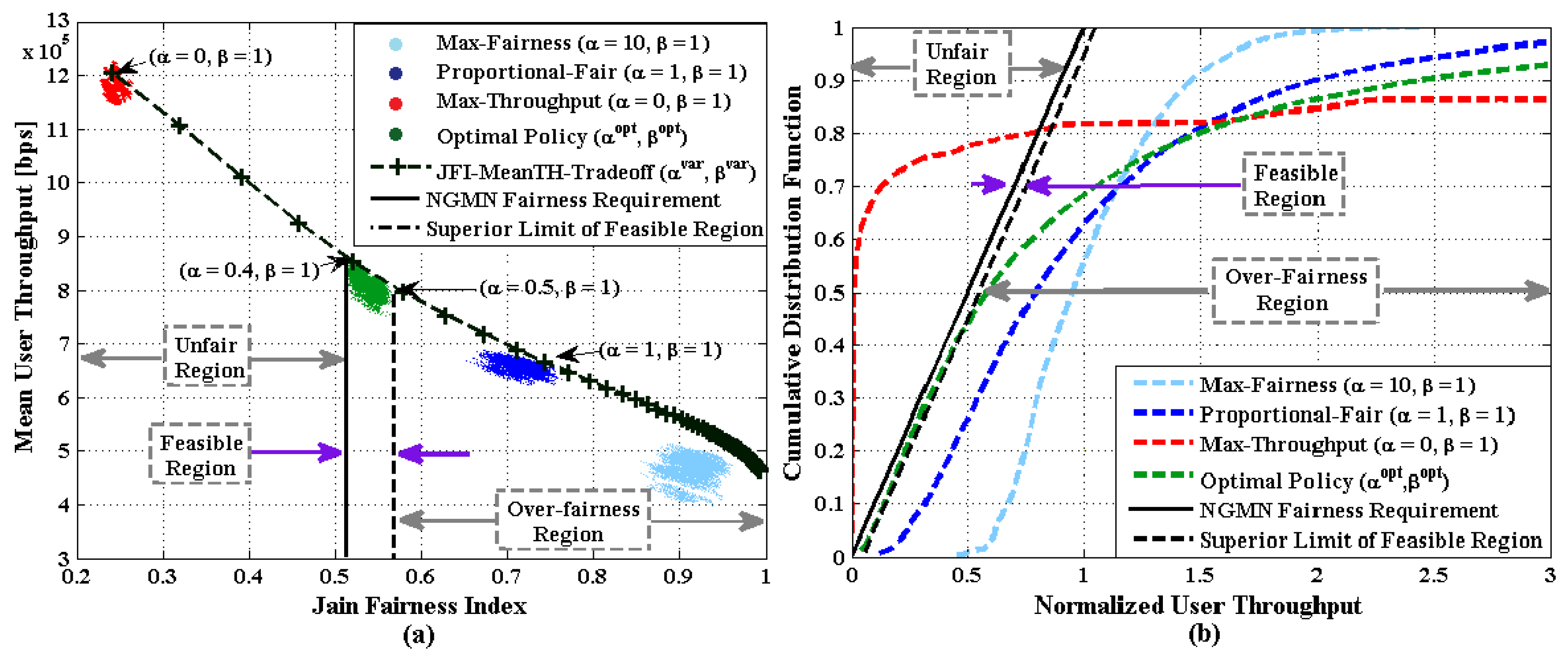
Figure 1. Trade-off concept of system throughput and user fairness [5]: (a) quantitative evaluation; (b) qualitative evaluation.
Information 10 00315 g001
Figure 2. Proposed System.
Information 10 00315 g002
Figure 3. Next Generation of Mobile Networks (NGMN) fairness evaluation based on exponential moving filter.
Information 10 00315 g003
Figure 4. Learning performance: (a) max/min distance reported to NGMN requirement; (b) ( α t , β t ) evolution.
Information 10 00315 g004
Figure 5. Fairness and throughput trade-off: (a) quantitative evaluation; (b) qualitative evaluation.
Information 10 00315 g005
Figure 6. CACLA-2 vs. other RL Candidates: (a) ρ = 2.0 ; (b) ρ = 2.25 ; (c) ρ = 2.5 ; (d) ρ = 3.0 ; (e) ρ = 4.0 ; (f) ρ = 4.25 (g) ρ = 4.5 ; (h) ρ = 5.0 ; and (i) ρ = 5.5 .
Information 10 00315 g006
Figure 7. System performance of the proposed CACLA-2 framework and state-of-the-art schedulers.
Information 10 00315 g007
Table 1. Simulation settings.
ParameterValue
System Bandwidth/Cell Radius20 MHz (100 RBs)/1000 m
User Speed/Mobility Model120 Kmph/Random Direction
Channel ModelJakes Model
Path Loss/Penetration LossMacro Cell Model/10 dB
Interfered Cells/Shadowing STD6/8 dB
Carrier Frequency/DL Power2 GHz/43 dBm
Frame StructureFDD
CQI Reporting ModeFull-band, periodic at each TTI
Physical Uplink Control CHannel
(PUCCH) ModelErrorless
Scheduler TypesSP-GPF, DP-GPF, MT [28], AS [29], RL Policies
Traffic TypeFull Buffer
No. of schedulable users U m a x 10 each TTI
RLC Automatic Repeat reQuest (ARQ)Transmission Mode
Adaptive Modulation and Coding
(AMC) LevelsQPSK, 16-QAM, 64-QAM
Target Block Error Rate (BLER)10%
Number of Users ( | U t | ) Variable: 15-120
RL AlgorithmsQ-Learning [12], Double-Q-Learning [41], SARSA [42], QV [43], QV2 [44], QVMAX [44], QVMAX2 [44], ACLA [38], CACLA-1 [45], CACLA-2 [45]
Exploration (learning and ER)/Exploitation4000 s (1000 s ER)/200 s for Q, DQ, and SARSA 3000 s/200 s for actor-critic RL
Forgetting factor ( ψ ), windowing Factor ( ρ ) β = 0.01 , ρ [ 2 ; 5.5 ]
Table 2. Controller parameters.
RL Algs.Learning Rate ( η Q ) Learning Rate ( η V ) Discount Factor ( γ ) Exploration ( ϵ , τ )
Q-Learning 10 3 0.99 ϵ -greedy ϵ = 10 4
DQ-Learning 10 3 0.99 ϵ -greedy ϵ = 10 4
SARSA 10 3 0.99Boltzmann τ = 10
QV 10 2 10 4 0.99Boltzmann τ = 1
QV2 10 3 10 5 0.95Boltzmann τ = 1
QVMAX 10 2 10 4 0.99Boltzmann τ = 10
QVMAX2 10 3 10 5 0.95Boltzmann τ = 1
ACLA 10 2 10 2 0.99 ϵ -greedy ϵ = 5 · 10 1
CACLA-1 10 2 10 2 0.99 ϵ -greedy ϵ = 5 · 10 1
CACLA-2 10 2 10 2 0.99 ϵ -greedy ϵ = 5 · 10 1