A Novel Multi-Criteria Decision-Making Model: Interval Rough SAW Method for Sustainable Supplier Selection


1
Faculty of Transport and Traffic Engineering Doboj, University of East Sarajevo, Vojvode Mišića 52, 74000 Doboj, Bosnia and Herzegovina
2
Faculty of Economics, University of Banja Luka, Majke Jugovića 4, 78000 Banja Luka, Bosnia and Herzegovina
3
Department of Logistics, Military Academy, University of Defence in Belgrade, Pavla Jurišića Sturma 33, 11000 Belgrade, Serbia
4
Department for Social Sciences, Institute for Scientific Research and Development Brcko district BiH, 76100 Brcko District, Bosnia and Herzegovina
*
Author to whom correspondence should be addressed.
Information 2019, 10(10), 292; https://doi.org/10.3390/info10100292
Submission received: 19 August 2019
/
Accepted: 19 September 2019
/
Published: 22 September 2019
(This article belongs to the Section Information Applications)
Abstract
:Sustainability in a supply chain is a demand on the one hand and a challenge on the other. It is necessary to balance between these dimensions in order to fulfill the purpose of the supply chain. Therefore, in the first phase—i.e., in procurement—it is necessary to take into account its sustainability. In this paper, a sustainable supplier was selected respecting all three aspects of sustainability. The evaluation was carried out on the basis of a total of 21 criteria arranged into two levels and three groups. A new Interval Rough SAW (simple additive weighting) method, which represents a contribution to the treatment of problems belonging to the multi-criteria decision-making (MCDM), was developed. The integration of interval rough numbers with the SAW method was completed. In addition, the full consistency method (FUCOM) was applied to determine the weights of the criteria. The integrated FUCOM-Interval Rough SAW model enables treatment of multi-criteria problems while reducing subjectivity to the lowest possible level and eliminating uncertainties and ambiguities. The results obtained were determined throughout a sensitivity analysis consisting of a change in the weight of the criteria and the influence of dynamic matrices on the change in ranks. In addition, Spearman’s rank correlation coefficient (SCC) was calculated to confirm the stability of the previously obtained results.
1. Introduction
Procurement of materials as a separate logistics sub-system plays an important role in achieving the efficiency of a sustainable supply chain and meeting its goals related to meeting the requirements of all participants. In the initial phase—i.e., in a procurement process—it is necessary to take into account adequate selection of suppliers, which will greatly influence the increase in competitiveness in the market. Suppliers are obliged to meet a number of requirements and be prepared to adapt their business policies to their customers at all times. In order to do this, it is necessary to consider all three aspects of sustainability: environmental, economic, and social. Accordingly, in this paper, the evaluation of suppliers has been performed considering 21 criteria from the aspect of all sustainability factors.
For this purpose, an integrated FUCOM-Interval Rough SAW model was developed. The FUCOM method was applied to determine the significance of the criteria arranged into two levels. First, the values of the main criteria, economic, social and environmental, were determined, and then the weights of all sub-criteria for each main group of criteria were calculated. Subsequently, the final values for all criteria were obtained by multiplying the values of the main criteria by the values of the sub-criteria for each group individually. The interval rough SAW method was developed and applied to rank and select suppliers from a potential set.
This paper has several aims. The first refers to the enrichment of the theory of multi-criteria problems, which is largely dominated by ambiguities and dilemmas. This aim is achieved by developing a novel interval rough SAW method. The second aim is to reduce subjectivity in group decision-making and to provide more precise determination of the preferences by decision-makers. This is achieved by integrating the FUCOM method and the developed interval rough SAW algorithm. The third aim is to optimize the procurement process—i.e., the evaluation and selection of a sustainable supplier in a lime manufacture company. The first two aims reflect the contribution of this research.
After the introduction, the paper is written throughout five more sections. The second section provides a comprehensive review of the literature, which consists of three parts: a review of the application of the FUCOM method, a review of published studies that have integrated rough set theory with MCDM methods, and a review of supplier selection over the past five years. The third section presents the model proposed in this study. The FUCOM algorithm is briefly given, as well as the significance and operations with interval rough numbers. The development of the interval rough SAW method is presented at the end of this section. The fourth section consists of the results where the calculation is shown in detail using the proposed integrated model. A sensitivity analysis that includes changing the weight of the criteria throughout a total of 21 scenarios and the impact of dynamic matrices on the rank change is performed in the fifth section. Finally, the sixth section presents concluding considerations and guidelines for future research.
2. Literature Review
2.1. Review of Applying the FUCOM Method in Various Fields
The nature of criteria is not the same for all problems, and therefore appropriate weight coefficients should be assigned to the criteria. A novel full consistency method (FUCOM) has been proposed for the accurate determination of the weight coefficients of criteria by Pamučar et al. [1]. The FUCOM method offers an advantage over existing multi-criteria decision-making methods since it requires only (n−1) comparison of criteria. The integrated FUCOM-MAIRCA model was tested in a study [2] assessing road and rail level crossings in Serbia. The evaluation of crossings is performed throughout the assessment of seven criteria established on the basis of representative literature and expert surveys. The presented model allows for the consideration of subjectivity in a process of group decision-making throughout the linguistic assessment of evaluation criteria. By Prentkovskis et al. [3], a new Delphi-FUCOM-SERVQUAL methodology was developed for improving the process of measuring the quality of express post services. The evaluation of dimensions was performed by 70 respondents, regular customers of services and customers who used services on a one-time basis. The advantage of the developed methodology is the fact that it enables accurate processing of input and output parameters and provides more objective results. Then, Nunić [4] applied the FUCOM method in estimating the weights of criteria with MABAC for the assessment of PVC joinery. Five potential manufacturers are evaluated on the basis of seven criteria. To select AGV as one important type of material handling equipment in a warehouse, Zavadskas et al. [5] used the integration of a new R-ROV model with the FUCOM method. A multi-criteria model was created on the basis of which a selection among nine AGVs was made and the FUCOM method was used to obtain the weights of seven criteria. In their paper, Fazlollahtabar et al. [6] presented the FUCOM method in group decision-making to evaluate an adequate forklift. The selection of a side-loading forklift is conditioned by the optimality of seven criteria required by working conditions to achieve the efficiency of the company’s storage system. Bozanic et al. [7] uses the FUCOM-FAZZY MABAC model to decide on the most appropriate location for a bridge, since proper location selection can prevent potential problems in the process of designing and subsequently using a single-span Bailey bridge. The advantages of the FUCOM method in comparison with the AHP method were demonstrated in a study [8] estimating Libyan airlines. The comparison was made on the basis of 16 key indicators arranged into 5 groups: reliability, management, employees, satisfaction, and tangibility. The model can be used as a decision-making support tool to improve the performance of airlines. The study [9] selected the optimal route criteria for the transport of hazardous materials using a new approach in the field of multi-criteria decision-making. The weight coefficients of these criteria were determined using the FUCOM method, and the evaluation and selection of suppliers was determined using the TOPSIS and MABAC methods. In the research paper [10], he presents the use of a multi-criteria FUCOM-WASPAS model for ranking dangerous road sections. The study covers seven traffic safety criteria that are evaluated by a linguistic scale. The same FUCOM-WASPAS model is used [11] to rank suppliers in a procurement system of a wood company. Considering that supplier selection is a key role for achieving a competitive advantage and reducing overall production costs, Matić et al. [12] apply a combined FUCOM-rough COPRAS model to estimate a sustainable supplier in a construction company. Durmić [13] also uses the FUCOM method to determine the significance of the criteria for selecting a sustainable supplier at two decision-making levels, with the first level consisting of three criteria: economic, social, and environmental, and the second level consisting of 21 sub-criteria. The results of the weight values of the criteria will be applied in this research study.
2.2. Review of Applying Multi-Criteria Methods in the Integration with Rough Numbers
More recently, rough set theory has been widely used in all fields with the integration of multi-criteria decision-making (MCDM) methods. The use of rough numbers together with MCDM methods, according to Stević et al. [14], provides good results and has numerous benefits. To ensure the satisfaction of all participants in the evaluation and selection of suppliers, Stević et al. [14] use a combination of rough numbers with MCDM methods: DEMATEL, EDAS, COPRAS, and MULTIMOORA, and compare the obtained results with rough MABAC and rough MAIRCA. In another study, Stević et al. [15] evaluate the supplier criteria in a wire manufacture company by applying the integration of rough sets with the analytic hierarchy process (AHP). The proposed approach shows that it offers the possibility of reducing costs, increasing competitiveness and achieving final-user satisfaction. In the paper by Shindpour et al. [16] for the evaluation of design concept, to address the uncertainties and ambiguities of the data in the primary stages of product design, the performance of design concepts is evaluated in relation to quantitative and qualitative criteria simultaneously using a rough set and a fuzzy set. The AHP method was used to obtain the criterion weights, while the evaluation was performed using the TOPSIS method. Tiwari et al. [17] evaluate the concept of design as a complex multi-criteria decision-making process by applying rough sets and the VIKOR method in order to reduce the imprecise content of the user evaluation process and thus improve the efficiency of product design. Zhu et al. [18] present a symmetric evaluation method by integrating an analytic hierarchy process based on rough numbers and the VIKOR method based on rough numbers to evaluate design in a subjective environment. The study [19] for solving multi-criteria problems proposes a bipolar model based on the integration of rough set theory and three-way decisions for forming a hybrid model. Karavidić and Projović [20] use rough sets in multi-criteria decision-making models to make decisions in operations of security forces. Such a model based on rough sets formulates specific decision-making rules that help decision-makers in a process of security operation planning. For the financial modeling and improvement planning of the life insurance industry, Shen et al. [21] propose a two-stage hybrid approach, where rough financial knowledge is retrieved first and then obtained core attributes are measured and synthesized using fuzzy-integral-based decision methods. Five companies were surveyed to illustrate the planning for financial performance improvement by applying this approach. When selecting suppliers in a PVC joinery company, Stojić et al. [22] use the rough AHP method to calculate the relative values of weight criteria, while the supplier assessment and ranking is conducted using the rough WASPAS method. In their paper, Zavadskas et al. [23] develop a new multi-criteria approach Rough Step-Wise Weight Assessment Ratio Analysis (R-SWARA) and demonstrate its application in logistics. To measure the performance of a Turkish airline, it is necessary to use a methodology considering quantitative and qualitative factors and their interrelationships, and for this reason the study [24] used an integral approach of the analytic hierarchy process enhanced by rough set theory. Additionally, fuzzy TOPSIS was used to obtain the final performance ranking. Kusi-Sarpong et al. [25] also use a new multi-criteria approach that integrates elements of rough set theory and fuzzy TOPSIS methodology to manage green supply chains in the mining industry. Rough sets in combination with the TOPSIS method are also applied by Song et al. [26] to analyze the modes and effects of failure in uncertain environments. The study [27] of the game evaluation model provides an integration of rough number theory with the fuzzy Delphi-AHP-TOPSIS model, where fuzzy Delphi is used to select evaluation criteria, fuzzy AHP is used to analyze the structure of criteria and determine the weights of criteria, and finally fuzzy TOPSIS is used to determine the order of evaluation. The successful integration of RST technique and the TOPSIS multi-criteria decision-making method by Khan et al. [28] led to the successful prediction of sites for the case of Pakistan Red Crescent Society (PRCS) in four districts examined. To evaluate 20 criteria divided into four sets, Vasiljević et al. [29] use AHP based on rough numbers. The proposed evaluation methodology was demonstrated throughout the application in a company that manufactures metal washers for the automotive industry. For the evaluation of university websites, Pamučar et al. [30] present the hybrid IR-AHP–MABAC (interval rough analytic hierarchy process–multiattributive border approximation area comparison) model adapted to group decision-making based on the application of a new approach to treating uncertainties using interval rough numbers.
2.3. Selection of Suppliers over the Last Five Years
Evaluating and selecting suppliers is one of the most important processes for achieving an efficient supply chain. Maintaining long-term partnerships with suppliers and using fewer reliable suppliers can help to increase the value of the supply chain [31]. Suppliers are a large part of a production process, accordingly they need to be sorted and carefully analyzed using an efficient framework [32]. In order to achieve the company’s sustainable development, the selection of a sustainable supplier in supply chains is made on the basis of an integrated AHP-VIKOR model [33]. The results show that environmental costs, quality of product, price of product, occupational health and safety systems, and environmental competencies have been ranked as the top five sustainable supplier selection criteria. Awasthi et al. [34] also use the VIKOR method for evaluating supplier performance but in integration with the fuzzy AHP method for generating criterion weights. This integrated approach considers sustainability risks from sub-suppliers (i.e., (1+n)th-tier suppliers). The study [35] proposes a FAHP-based supplier selection model for the automobile industry that often faces a heterogeneous supply environment. Azimifard et al. [36] present an integrated approach of AHP and TOPSIS methods at three levels to select sustainable supplier countries for the Iranian steel industry. In [37], the selection of suppliers for a steel manufacture company in Libya is based on the application of the CODAS method. Recognizing the importance of a supplier selection decision that significantly influences its competitive market position, the authors Rezaei et al. [38] propose an innovative methodology for selecting suppliers throughout three phases: pre-selection, selection, and aggregation. For the supplier selection phase, the authors use the best worst method (BWM). Karsak and Dursun [39] develop a multi-criteria approach using the QFD method for supplier selection. Azadnia el al. [40] present an integrated approach of weighted rule-based fuzzy method, fuzzy analytic hierarchy process and multi-objective mathematical programming to select a sustainable supplier for the case study of packaging foils in the food industry. Girubha et al. [41] compare two ISM-ANP-ELECTRE and ISM-ANP-VIKOR models for the problem of sustainable supplier selection. In order to make supplier selection in terms of sustainability, Arabsheybani et al. [32] apply the fuzzy MOORA model and use the FMEA technique to evaluate supplier risk. The authors Öztürk and Özçelik [42] model the supplier selection problem in the context of a sustainable supply chain based on the triple bottom concept. Due to the multi-criteria nature, the fuzzy TOPSIS method is applied to the sustainable supplier selection of an energy company. Mehregan et al. [43] illustrate how an integrated interpretive structural modeling (ISM) and fuzzy DEMATEL approach can be a valuable management tool for evaluating and analyzing interactions among criteria. The feasibility and effectiveness of this approach is illustrated by the Iranian Gas Engineering and Development Company (IGEDC). The paper [44] framed 12 criteria from an economic, environmental, and social perspective for evaluating suppliers using the TOPSIS method. A novel hierarchical grey-DEMATEL approach is used to improve sustainable supply chain management in the study [45]. The purpose of this study is to apply grey theory that compensates for incomplete information and hierarchical structures to identify aspects of and criteria for supplier prioritization. Moohamed et al. [46] present a sustainable supplier problem-solving framework based on the application of four methods: AHP, fuzzy TOPSIS, MOPM, and TOPSIS.
3. Methods
Figure 1 shows the proposed methodology consisting of four phases and 14 steps. The first phase represents the initial research and data collection and consists of five steps. The first step defines the necessity for research, followed by the definition of research aims in the second step. Then, an MCDM model has been formed, consisting of three main criteria that consider all three aspects of sustainability and a total of 21 sub-criteria equally classified into all three categories. The fourth step of the first phase is data collection, and the fifth step is the assessment of criteria, sub-criteria, and alternatives by a decision-making team. The second phase includes the development of methodology that represents the basic scientific contribution of this paper. After sorting and preparing the data for calculation, a novel interval rough SAW algorithm has been developed, which is presented in detail below. In addition, an integrated model has been created on the basis of applying the FUCOM method and developed interval rough SAW method. The third phase includes a case study in which a sustainable supplier has been selected. The FUCOM method has been applied to calculate the weights of criteria, after which the transformation of individual matrices into interval rough matrices is performed. At the end of this phase, the ranking of suppliers is performed using the developed interval rough SAW algorithm. In the fourth phase, a sensitivity analysis, i.e., validation of the obtained results, is performed in three steps. First, the significance of the criteria is changed and 21 scenarios are created. Subsequently, in the second step, the influence of dynamic matrices on rank reversal is tested, and at the end of the sensitivity analysis, the results obtained are compared using the interval rough COPRAS method.
3.1. Full Consistency Method (FUCOM)
One of the new methods that is based on the principles of pairwise comparison and validation of results through deviation from maximum consistency is the full consistency method (FUCOM) [1]. Benefits that are determinative for the application of FUCOM are a small number of pairwise comparisons of criteria (only n-1 comparison), the ability to validate the results by defining the deviation from maximum consistency (DMC) of comparison and appreciating transitivity in pairwise comparisons of criteria. The FUCOM model also has a subjective influence of a decision-maker on the final values of the weights of criteria. This particularly refers to the first and second steps of FUCOM in which decision-makers rank the criteria according to their personal preferences and perform pairwise comparisons of ranked criteria. However, unlike other subjective models, FUCOM has shown minor deviations in the obtained values of the weights of criteria from optimal values [1]. Additionally, the methodological procedure of FUCOM eliminates the problem of redundancy of pairwise comparisons of criteria, which exists in some subjective models for determining the weights of criteria.
Assume that there are n evaluation criteria in a multi-criteria model that are designated as wj, j = 1,2, ..., n, and that their weight coefficients need to be determined. Subjective models for determining weights based on pairwise comparison of criteria require a decision-maker to determine the degree of impact of the criterion i on the criterion j. In accordance with the defined settings, Figure 2 presents the FUCOM algorithm [1].
3.2. Interval Rough Numbers
The process of group decision-making is accompanied by a great amount of uncertainty and subjectivity, so decision-makers often have dilemmas when assigning certain values to decision attributes. In this paper, a new approach in the theory of rough sets, an approach based on interval rough numbers (IRN), is applied to process the uncertainty contained in data in group decision-making. Suppose that one decision attribute should be assigned a value presented by a qualitative scale whose values range from 1 to 5. One decision-maker (DM) may consider that the decision attribute should have a value between 3 and 4, another DM may consider that a value between 4 and 5 should be assigned, while the third DM has no dilemma about the value of the decision attribute and assigns a value of 4. The dilemmas presented are extremely common in a group decision-making process. In such situations, one of the solutions is to geometrically average two values between which individual decision-makers are in doubt. However, in such situations, the uncertainty (ambiguity) that prevailed in a decision-making process would be lost and further calculation would be reduced to crisp values. On the other hand, the use of fuzzy or grey techniques would entail predicting the existence of uncertainty and subjectively defining the interval by which uncertainty is exploited. Subjectively defined intervals in further data processing can significantly influence the final decision [47], which should definitely be avoided if we aim at impartial decision-making.
On the contrary, the approach based on interval rough numbers includes exploiting the uncertainty that exists in the data obtained. By applying the arithmetic operations that are explained in the following section, we obtain the values of attributes that fully describe the specified uncertainties without subjectively affecting their values. Thus, the uncertainties of the first DM can be described by an interval rough number IRN = [(3,3.67), (4,4.33)], of the second DM by IRN = [(3.67,4), (4.33,5)], while of the third DM by IRN = [(3.67,4), (4,4.33)]. A detailed procedure for determining IRN is explained in the following section.
Suppose that there is a set of classes that represent the preferences of DM, , provided that they belong to a sequence that satisfies the condition and the second set of classes that also represent the preferences of DM, . All objects are defined in the universe and related to the preferences of DM. In , each class of objects is presented in an interval , where the condition that () is satisfied, as well as the condition that . Then represents the lower limit of the interval, while represents the upper limit of the interval of th class of objects. If both limits of the object classes (upper and lower limit) are arranged in such a way that (), respectively, then we can define two new sets that contain the lower object class and upper object class , respectively. Then for any class of objects () and (), we can define the lower approximation of and as
The upper approximations of and are defined by applying the following expressions
Both classes of objects (upper and lower class of objects and ) are defined by their lower limits and and upper limits and , respectively,
where and represent the total number of objects contained in the lower approximation of the classes of objects and , respectively. The upper limits and are defined by Expressions (7) and (8)
where and represent the total number of objects contained in the upper approximation of the classes of objects and , respectively.
For the lower class of objects, rough boundary interval of is presented as and denotes the interval between the lower and upper limit
Whereas for the upper class of objects, we obtain the rough boundary interval of as
Then the uncertain class of objects and can be presented using their lower and upper limits
As we can see, each class of objects is defined by its lower and upper limits that represent the interval rough number, which is defined as
The procedure for determining IRN will be explained by the example of determining the weight coefficient of criterion wi in which four experts participate. The experts evaluated the criteria using a scale that encompasses integer values in the interval from one to five: 1—very small impact; 2—small impact; 3—medium impact; 4—large impact; and 5—very large impact. The experts’ evaluations are shown in Table 1.
The experts’ evaluations in Table 1 are presented in the form of ordered pairs (ai;bi), where ai and bi are the values assigned by the experts to the criteria from scale 1–5. The experts who cannot confidently opt for one of the values in the scale, enter both values that they have a dilemma about (E1, E2, and E3). In our example, only the expert E4 had no dilemma and chose a unique value from the scale.
These uncertainties can be represented by trapezoidal fuzzy numbers of the form A = (a1, a2, a3, a4), where a2 and a3 represent values in which the membership function reaches its maximum value, while a1 and a4 represent the left and right limit of the fuzzy set, respectively. In our example (Table 1), we obtain four trapezoidal fuzzy numbers A (E1) = (1,2,3,4), A (E2) = (2,3,4,5), A (E3) = (3. 4,5,5), and A (E4) = (4,5,5,5). Trapezoidal fuzzy numbers are graphically shown in Figure 3, where a darker nuance indicates values in which the membership function reaches its maximum value (a2 and a3), while a light nuance indicates elements of a set that more or less belong to the fuzzy set (a1 and a4).
In addition to the fuzzy approach, the uncertainties described can also be presented by interval rough numbers. Since in the previous section, Expressions (1)–(12), it is defined that an IRN consists of two rough sequences and we distinguish two classes of objects wi and w’i: and . Using Expressions (1)–(8), rough sequences (11) and (12) are formed for each class of objects. For the first class of objects, we obtain:
, ;
, ;
, ;
, ;
For the second class of objects, we obtain:
, ;
, ;
, ;
On the basis of rough sequences, we obtain interval rough numbers: , , and .
By rational reasoning, without applying rough and fuzzy sets, we conclude that the values of the criterion wi should be between the values of 3.5 and 4.25. These values are obtained by geometrical averaging the classes of objects and . In Figure 3, the rational (expected) values of 3.5 and 4.25 are shown by the dashed line. From Figure 3, we can see that the expected values (3.5 and 4.25) are completely within all IRNs. On the other hand, fuzzy numbers only partially cover expected values. The affiliation function of fuzzy numbers A(E2) and A(E3) with maximum affiliation only partially covers the expected values, while the fuzzy numbers A(E1) and A(E4) cover the expected values with an affiliation degree of 0.5. On the other hand, all IRNs fully cover the expected values (3.5 and 4.25) by their intervals.
Interval rough numbers are characterized by specific arithmetic operations, which are different from arithmetic operations with classical rough numbers. Arithmetic operations between two interval rough numbers and are performed using Expressions (14), (15), (16), (17), and (18):
(1) Addition of interval rough numbers, “+”,
(2) Subtraction of interval rough numbers, “−”,
(3) Multiplication of interval rough numbers, “×”,
(4) Division of interval rough numbers, “/”,
(5) Scalar multiplication of interval rough numbers where
Any two interval rough numbers and are ranked according to the following rules:
(1) If the interval of interval rough number is not strictly bounded by another interval, then:
(a) If the condition that { i } or { i } is satisfied, then , Figure 4a.
(b) If the condition that { and } is satisfied, then , Figure 4b.
(2) If the intervals of interval rough numbers and are strictly bounded, then it is necessary to determine the intersection points and of interval rough numbers and . If the condition that and is satisfied, then:
(c) If the condition that is satisfied, then , Figure 4c,d.
(d) If the condition that is satisfied, then , Figure 4e.
The intersection points of interval rough numbers are obtained in the following way:
3.3. Interval Rough SAW Method
The SAW method is a simple and easily applicable method of multi-criteria decision-making. However, using only crisp numbers it is impossible to obtain results that treat uncertainty and objectivity in an adequate way [48]. The rough SAW method was developed two years ago and presented in study [48]. This paper presenting a new approach that combines the SAW method and interval rough numbers consists of the following steps:
Step 1: Forming a multi-criteria decision-making model that consists of m alternatives and n criteria.
Step 2: Forming a team of r experts, who will make assessment of the alternatives according to all the criteria and sub-criteria.
Step 3: Transformation of individual matrices into a group interval rough matrix. In this step, it is necessary to transform each individual matrix of experts r1, r2, ..., rn into an interval rough group matrix using Equations (1)–(12)
where m denotes a number of alternatives and n denotes a number of criteria.
Step 4: Normalization of the initial interval rough group matrix (24) using Equations (25) and (26):
If the criterion belongs to the benefit group, then Equation (25) is used for the normalization process
Whereas for the criteria belonging to the cost group, Equation (26) is applied
Equations (25) and (26) are further broken down in Equations (27) and (28)
Step 5: Weighting the previous normalized matrix
Step 6: Summing all of the values of the alternatives obtained (summing by rows)
Step 7: Ranking the alternatives in descending order, that is, the highest value is the best alternative. In order to rank the potential solutions more easily, the rough number can be converted into a crisp number using the average value.
4. Results
The selection of a sustainable supplier depends on the precise determination and selection of appropriate criteria and their evaluation. Criteria and alternatives were evaluated by a group of employed experts according to the requirements of Carmeuse (Bosnia and Herzegovina), a lime manufacture company. This group consists of three decision-makers. The criteria for selecting a sustainable supplier are as follows:
- Sub-criteria of the group of economic criteria C1: C11—cost / price; C12—quality; C13—flexibility; C14—productivity; C15—financial capacity; C16—partnerships; and C17—ecological innovations
- Sub-criteria of the group of social criteria C2: C21—reputation; C22—work safety; C23—employees’ rights; C24—local community influence; C25—training of employees; C26—respect for rights and policies; and C27—release of information.
- Sub-criteria of the group of environmental criteria C3: C31 — environmental image; C32—recycling; C33—pollution control; C34—environmental management system; C35—environmentally friendly products; C36—resource consumption; and C37—green competencies.
The complete calculation of the criteria is shown in [13], where the following values of criteria are obtained, which are further used in the calculation with the Interval Rough SAW method:
The evaluation of alternatives by three decision-makers has been performed using interval numbers as shown in Table 2.
Applying Equations (1)–(12), the values from Table 2 are transformed into interval rough values, which represent the initial interval rough matrix shown in Table 3.
Then, Equations (24)–(28) need to be applied to normalize the initial interval rough matrix. Criteria C11 and C36 belong to the cost group, while the other criteria need to be maximized, i.e., they belong to the group of beneficial criteria. Table 4 shows the normalized interval rough matrix.
An example of calculating a normalized matrix for the criteria belonging to the cost group is:
for the alternative A1.
An example of calculating a normalized matrix for the criteria belonging to the benefit group is:
for the alternative A4.
Subsequently, the normalized interval rough matrix is weighted with the criterion values obtained using the FUCOM method. The weighting is performed by applying Equation (29), while summing the values for alternatives by rows is obtained by applying Equation (30). Table 5 shows the final results of an integrated FUCOM–interval rough SAW approach.
Ranking is performed in descending order, with the highest value being the best solution and the lowest being the worst. Alternative 4 is the most acceptable solution according to the results obtained.
5. Sensitivity Analysis
5.1. Changing the Weights of Criteria
The purpose of sensitivity analysis is to evaluate the impact of the most influential criterion on the ranking performance of the proposed model. After determining the weight coefficients of the criteria using FUCOM, the “most important criterion” is identified for the purpose of sensitivity analysis. Based on the recommendations by Kirkvood [49] and Kahraman [50], Equation (31) is defined, expressing the proportionality of weights during the analysis of sensitivity
where represents the change in the weights of the criteria in the sensitivity analysis, represents the weight of the most significant criterion, represents the original values of the weights of the criteria, and represents the sum of the original weight values of the criteria being changed. The parameter is defined as the weight coefficient of elasticity, which expresses the relative compensation of other weight coefficient values with respect to the given changes in the weight of the most significant criterion [49,50].
The assumptions made when conducting the sensitivity analysis are as follows [50]: (a) The value of the elasticity weight coefficient for the most significant criterion is defined as one; (b) The ratio of variable weights remains constant throughout the sensitivity analysis. The parameter (Expression (31)) represents the amount of change that is applied to a set of weight coefficients depending on their elasticity weight coefficients. The change in the weights of the most important criterion should be restricted. Otherwise, the weights may take negative values, which would violate the constraints of weight proportionality. The parameter can be (a) positive, indicating an increase in relative importance, or (b) negative, indicating a decrease in relative importance. The limits for are defined as the largest change in weight of the most significant criterion in the negative and positive direction, i.e., . After defining the limits for , the new weights of criteria are calculated according to the previously set parameters for the sensitivity analysis. A new set of criteria always satisfies the universal state of proportionality of the weight coefficients that [50]. Based on the new criterion values obtained, the ranks of the alternatives for the observed scenario are calculated.
In this research, criterion C2 has been identified as the most influential, since it has the highest value of the weight coefficient . In the next step, the elasticity weight coefficient () of the most significant criterion is determined (Table 6) and the limits of change in the weight coefficient of the most significant criterion () are defined.
Thus, the boundary values of criterion C2, which are [−0.135, 0.865], are obtained. Based on the defined limits of change in the weight coefficient of the most significant criterion, the scenarios for the sensitivity analysis are determined by dividing the interval −0.135≤≤0.865 into a total of 21 scenarios. Thus, the new values of the weight coefficients for 21 scenarios are defined, Table 7.
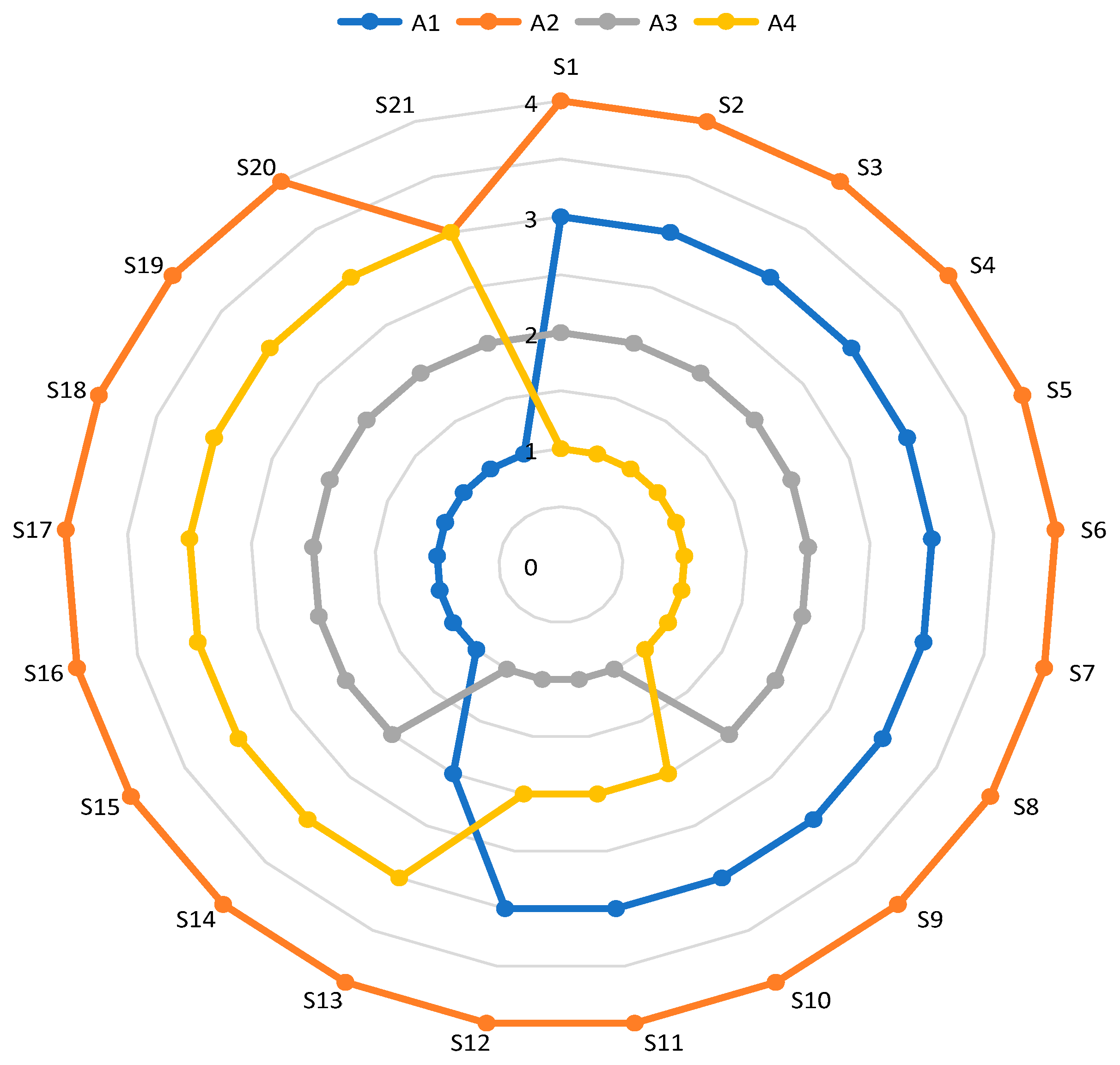
The effect of the new values of weight coefficients (Table 7) on the change in the ranks of alternatives is shown in Figure 5.
The results (Figure 5) show that the rankings of considered alternatives change, thus confirming that the model is sensitive to changes in weight coefficients. By comparing the two top-ranked alternatives (A4 and A3) across the scenarios, we can conclude that the A4 alternative remained top-ranked in nine scenarios, while in the remaining scenarios it was second-ranked (in three scenarios) and third-ranked (in nine scenarios). In addition, the second-ranked alternative (A3) maintained its position in 17 scenarios, while it was ranked first in four scenarios. The other alternatives (A1 and A3) also changed rankings. In order to make a final decision regarding the robustness of the obtained solution, it is necessary to determine the statistical dependence of the changes. The statistical dependence of changes in rankings of alternatives across scenarios was determined using the Spearman’s correlation coefficient (SCC).
The results of SCC application show that there is an extremely high correlation between the initial rank and the first 12 scenarios, which is 0.950. In the remaining nine scenarios, the correlation decreases and the average value is 0.211. Since, in more than 57% of the scenarios, the top-ranked alternative (A4) retains its rank and is ranked second or third in the remaining scenarios, we can conclude that there is a satisfactory rank correlation and that the proposed rank is confirmed and credible.
5.2. Influence of Dynamic Matrices on Rank Change
Changing certain parameters of decision matrix, such as introducing a new alternative or eliminating the existing one, can lead to changes in preferences. Therefore, in the following part, several scenarios have been formed where the change in decision matrix elements is simulated. Scenarios have been formed so that the worst alternative is eliminated from subsequent considerations in each scenario. At the same time, the remaining alternatives are ranked for each scenario according to the new initial decision-making matrix. This analysis has two goals: (1) to consider the robustness of the obtained solution under uncertain conditions; and (2) to analyze the performance of the IRN SAW model under the conditions of a dynamic initial decision matrix.
The initial solution using the IRN SAW model was generated as A4 > A3 > A1 > A2. The alternative A2 was identified as the worst, so in the first scenario it was eliminated from the set. Thus, a new decision matrix was obtained with a total of three alternatives. A new solution was generated and the following preferences A4>A3>A1 were obtained. The preferences from the first scenario show that A4 is still the best alternative, while A1 is the worst alternative. In the following scenario, alterative A1 was eliminated and the following rank A4>A3 was obtained. From the results presented, we can conclude that the A4 alternative remains the best-ranked across all the scenarios, thus confirming the robustness of the obtained ranks in a dynamic environment.
6. Conclusions
In this paper, the interval rough SAW method has been developed, which represents a major contribution. With the development of this method, it is possible to treat problems with multiple criteria in a more precise way, considering the uncertainties and ambiguities that are certainly part of solving such problems. Integration with interval numbers and the application of rough set theory results in a model that satisfies various aspects of optimization. In addition, the integration with the FUCOM method has been performed, which allows for reduction of subjectivity in determining the weight of criteria.
The integrated FUCOM–interval rough SAW model was applied to evaluate a sustainable supplier based on 21 criteria arranged into a two-level hierarchical structure. The criteria that equally support all three aspects of sustainability were involved. The FUCOM method was applied to determine the significance of the criteria. First, the values of the main criteria, economic, social, and environmental, were determined, and then the weights of all sub-criteria for each main group of criteria were calculated. The interval rough SAW method was developed and applied to rank and select suppliers from a potential set. The results obtained show that the fourth supplier is the best solution. The validity of the final results was determined throughout a sensitivity analysis. In the sensitivity analysis, 21 scenarios were formed first, which involved changing the weight of the criteria. Subsequently, the influence of dynamic matrices on the ranks of alternatives was tested, and it was identified that there was no change in ranks. The results were also compared with the interval rough COPRAS method [51], which also confirmed the previous results.
Future research related to this paper refers to the integration of other MCDM methods with interval rough numbers when it comes to the methodology applied. In addition, it is possible to identify an extension of the set of criteria for the supplier evaluation from the practical aspect.
Author Contributions
Conceptualization, M.G.; Data curation, E.D.; Formal analysis, A.P. Methodology, Ž.S.; Validation, D.P.; Writing—Original Draft, Ž.S. and E.D.; Writing—Review & Editing, M.G. and D.P.
Funding
This research received no external funding.
Conflicts of Interest
The authors declare no conflict of interest.
References
- Pamučar, D.; Stević, Ž.; Sremac, S. A new model for determining weight coefficients of criteria in mcdm models: Full consistency method (fucom). Symmetry 2018, 10, 393. [Google Scholar] [CrossRef]
- Pamučar, D.; Lukovac, V.; Božanić, D.; Komazec, N. Multi-criteria FUCOM-MAIRCA model for the evaluation of level crossings: Case study in the Republic of Serbia. Oper. Res. Eng. Sci. Theory Appl. 2018, 1, 108–129. [Google Scholar] [CrossRef]
- Prentkovskis, O.; Erceg, Ž.; Stević, Ž.; Tanackov, I.; Vasiljević, M.; Gavranović, M. A new methodology for improving service quality measurement: Delphi-FUCOM-SERVQUAL model. Symmetry 2018, 10, 757. [Google Scholar] [CrossRef]
- Nunić, Z. Evaluation and selection of Manufacturer PVC carpentry using FUCOM-MABAC model. Oper. Res. Eng. Sci. Theory Appl. 2018, 1, 13–28. [Google Scholar] [CrossRef]
- Zavadskas, E.K.; Nunić, Z.; Stjepanović, Ž.; Prentkovskis, O. A novel rough range of value method (R-ROV) for selecting automatically guided vehicles (AGVs). Stud. Inform. Control 2018, 27, 385–394. [Google Scholar] [CrossRef]
- Fazlollahtabar, H.; Smailbašić, A.; Stević, Ž. FUCOM method in group decision-making: Selection of forklift in a warehouse. Decis. Mak. Appl. Manag. Eng. 2019, 2, 49–65. [Google Scholar] [CrossRef]
- Bozanic, D.; Tešić, D.; Kočić, J. Multi-criteria FUCOM-Fuzzy MABAC model for the selection of location for construction of single-span bailey bridge. Decis. Mak. Appl. Manag. Eng. 2019, 2, 132–146. [Google Scholar] [CrossRef]
- Badi, I.; Abdulshahed, A. Ranking the Libyan airlines by using full consistency method (FUCOM) and analytical hierarchy process (AHP). Oper. Res. Eng. Sci. Theory Appl. 2019, 2, 1–14. [Google Scholar] [CrossRef]
- Noureddine, M.; Ristic, M. Route planning for hazardous materials transportation: Multicriteria decision making approach. Decis. Mak. Appl. Manag. Eng. 2019, 2, 66–85. [Google Scholar] [CrossRef]
- Nenadić, D. Ranking dangerous sections of the road using MCDM model. Decis. Mak. Appl. Manag. Eng. 2019, 2, 115–131. [Google Scholar] [CrossRef]
- Erceg, Ž.; Mularifović, F. Integrated MCDM model for processes optimization in supply chain management in wood company. Oper. Res. Eng. Sci. Theory Appl. 2019, 2, 37–50. [Google Scholar] [CrossRef]
- Matić, B.; Jovanović, S.; Das, D.K.; Zavadskas, E.K.; Stević, Ž.; Sremac, S.; Marinković, M. A New Hybrid MCDM Model: Sustainable Supplier Selection in a Construction Company. Symmetry 2019, 11, 353. [Google Scholar] [CrossRef]
- Durmić, E. Evaluation of criteria for sustainable supplier selection using FUCOM method. Oper. Res. Eng. Sci. Theory Appl. 2019, 2, 91–107. [Google Scholar] [CrossRef]
- Stević, Ž.; Pamučar, D.; Vasiljević, M.; Stojić, G.; Korica, S. Novel integrated multi-criteria model for supplier selection: Case study construction company. Symmetry 2017, 9, 279. [Google Scholar] [CrossRef]
- Stević, Ž.; Tanackov, I.; Vasiljević, M.; Rikalović, A. Supplier evaluation criteria: AHP rough approach. In Proceedings of the XVII International Scientific Conference on Industrial Systems, Novi Sad, Serbia, 4–6 October 2017; pp. 298–303. [Google Scholar]
- Shidpour, H.; Da Cunha, C.; Bernard, A. Group multi-criteria design concept evaluation using combined rough set theory and fuzzy set theory. Expert Syst. Appl. 2016, 64, 633–644. [Google Scholar] [CrossRef]
- Tiwari, V.; Jain, P.K.; Tandon, P. Product design concept evaluation using rough sets and VIKOR method. Adv. Eng. Inform. 2016, 30, 16–25. [Google Scholar] [CrossRef]
- Zhu, G.N.; Hu, J.; Qi, J.; Gu, C.C.; Peng, Y.H. An integrated AHP and VIKOR for design concept evaluation based on rough number. Adv. Eng. Inform. 2015, 29, 408–418. [Google Scholar] [CrossRef]
- Shen, K.Y.; Tzeng, G.H. A novel bipolar MCDM model using rough sets and three-way decisions for decision aids. In Proceedings of the 2016 Joint 8th International Conference on Soft Computing and Intelligent Systems (SCIS) and 17th International Symposium on Advanced Intelligent Systems (ISIS), Sapporo, Japan, 25–28 August 2016; pp. 53–58. [Google Scholar]
- Karavidić, Z.; Projović, D. A multi-criteria decision-making (MCDM) model in the security forces operations based on rough sets. Decis. Mak. Appl. Manag. Eng. 2018, 1, 97–120. [Google Scholar] [CrossRef]
- Shen, K.Y.; Hu, S.K.; Tzeng, G.H. Financial modeling and improvement planning for the life insurance industry by using a rough knowledge based hybrid MCDM model. Inf. Sci. 2017, 375, 296–313. [Google Scholar] [CrossRef]
- Stojić, G.; Stević, Ž.; Antuchevičienė, J.; Pamučar, D.; Vasiljević, M. A novel rough WASPAS approach for supplier selection in a company manufacturing PVC carpentry products. Information 2018, 9, 121. [Google Scholar] [CrossRef]
- Zavadskas, E.K.; Stević, Ž.; Tanackov, I.; Prentkovskis, O. A novel multicriteria approach-rough step-wise weight assessment ratio analysis method (R-SWARA) and its application in logistics. Stud. Inform. Control 2018, 27, 97–106. [Google Scholar] [CrossRef]
- Aydogan, E.K. Performance measurement model for Turkish aviation firms using the rough-AHP and TOPSIS methods under fuzzy environment. Expert Syst. Appl. 2011, 38, 3992–3998. [Google Scholar] [CrossRef]
- Kusi-Sarpong, S.; Bai, C.; Sarkis, J.; Wang, X. Green supply chain practices evaluation in the mining industry using a joint rough sets and fuzzy TOPSIS methodology. Resour. Policy 2015, 46, 86–100. [Google Scholar] [CrossRef]
- Song, W.; Ming, X.; Wu, Z.; Zhu, B. A rough TOPSIS approach for failure mode and effects analysis in uncertain environments. Qual. Reliab. Eng. Int. 2014, 30, 473–486. [Google Scholar] [CrossRef]
- Su, C.H.; Chen KT, K.; Fan, K.K. Rough set theory based fuzzy TOPSIS on serious game design evaluation framework. Math. Probl. Eng. 2013. [Google Scholar] [CrossRef]
- Khan, C.; Anwar, S.; Bashir, S.; Rauf, A.; Amin, A. Site selection for food distribution using rough set approach and TOPSIS method. J. Intell. Fuzzy Syst. 2015, 29, 2413–2419. [Google Scholar] [CrossRef] [Green Version]
- Vasiljević, M.; Fazlollahtabar, H.; Stević, Ž.; Vesković, S. A rough multicriteria approach for evaluation of the supplier criteria in automotive industry. Decis. Mak. Appl. Manag. Eng. 2018, 1, 82–96. [Google Scholar] [CrossRef]
- Pamučar, D.; Stević, Ž.; Zavadskas, E.K. Integration of interval rough AHP and interval rough MABAC methods for evaluating university web pages. Appl. Soft Comput. 2018, 67, 141–163. [Google Scholar] [CrossRef]
- Keshavarz Ghorabaee, M.; Amiri, M.; Zavadskas, E.K.; Antucheviciene, J. Supplier evaluation and selection in fuzzy environments: A review of MADM approaches. Econ. Res. Ekon. Istraživanja 2017, 30, 1073–1118. [Google Scholar] [CrossRef]
- Arabsheybani, A.; Paydar, M.M.; Safaei, A.S. An integrated fuzzy MOORA method and FMEA technique for sustainable supplier selection considering quantity discounts and supplier’s risk. J. Clean. Prod. 2018, 190, 577–591. [Google Scholar] [CrossRef]
- Luthra, S.; Govindan, K.; Kannan, D.; Mangla, S.K.; Garg, C.P. An integrated framework for sustainable supplier selection and evaluation in supply chains. J. Clean. Prod. 2017, 140, 1686–1698. [Google Scholar] [CrossRef]
- Awasthi, A.; Govindan, K.; Gold, S. Multi-tier sustainable global supplier selection using a fuzzy AHP-VIKOR based approach. Int. J. Prod. Econ. 2018, 195, 106–117. [Google Scholar] [CrossRef]
- Yadav, V.; Sharma, M.K. Multi-criteria decision making for supplier selection using fuzzy AHP approach. Benchmarking Int. J. 2015, 22, 1158–1174. [Google Scholar] [CrossRef]
- Azimifard, A.; Moosavirad, S.H.; Ariafar, S. Selecting sustainable supplier countries for Iran’s steel industry at three levels by using AHP and TOPSIS methods. Resour. Policy 2018, 57, 30–44. [Google Scholar] [CrossRef]
- Badi, I.; Abdulshahed, A.M.; Shetwan, A. A case study of supplier selection for a steelmaking company in Libya by using the Combinative Distance-based ASsessment (CODAS) model. Decis. Mak. Appl. Manag. Eng. 2018, 1, 1–12. [Google Scholar] [CrossRef]
- Rezaei, J.; Nispeling, T.; Sarkis, J.; Tavasszy, L. A supplier selection life cycle approach integrating traditional and environmental criteria using the best worst method. J. Clean. Prod. 2016, 135, 577–588. [Google Scholar] [CrossRef]
- Karsak, E.E.; Dursun, M. An integrated fuzzy MCDM approach for supplier evaluation and selection. Comput. Ind. Eng. 2015, 82, 82–93. [Google Scholar] [CrossRef]
- Azadnia, A.H.; Saman MZ, M.; Wong, K.Y. Sustainable supplier selection and order lot-sizing: An integrated multi-objective decision-making process. Int. J. Prod. Res. 2015, 53, 383–408. [Google Scholar] [CrossRef]
- Girubha, J.; Vinodh, S.; Kek, V. Application of interpretative structural modelling integrated multi criteria decision making methods for sustainable supplier selection. J. Model. Manag. 2016, 11, 358–388. [Google Scholar] [CrossRef]
- Öztürk, B.A.; Özçelik, F. Sustainable supplier selection with a fuzzy multi-criteria decision making method based on triple bottom line. Bus. Econ. Res. J. 2014, 5, 129. [Google Scholar]
- Mehregan, M.R.; Hashemi, S.H.; Karimi, A.; Merikhi, B. Analysis of interactions among sustainability supplier selection criteria using ISM and fuzzy DEMATEL. Int. J. Appl. Decis. Sci. 2014, 7, 270–294. [Google Scholar] [CrossRef]
- Jia, P.; Govindan, K.; Choi, T.M.; Rajendran, S. Supplier selection problems in fashion business operations with sustainability considerations. Sustainability 2015, 7, 1603–1619. [Google Scholar] [CrossRef]
- Su, C.M.; Horng, D.J.; Tseng, M.L.; Chiu, A.S.; Wu, K.J.; Chen, H.P. Improving sustainable supply chain management using a novel hierarchical grey-DEMATEL approach. J. Clean. Prod. 2016, 134, 469–481. [Google Scholar] [CrossRef]
- Mohammed, A.; Setchi, R.; Filip, M.; Harris, I.; Li, X. An integrated methodology for a sustainable two-stage supplier selection and order allocation problem. J. Clean. Prod. 2018, 192, 99–114. [Google Scholar] [CrossRef] [Green Version]
- Duntsch, I.; Gediga, G. The rough set engine GROBIAN. In Proceedings of the 15th IMACS World Congress, Berlin, Germany, 24–29 August 1997; pp. 613–618. [Google Scholar]
- Stević, Ž.; Pamučar, D.; Kazimieras Zavadskas, E.; Ćirović, G.; Prentkovskis, O. The selection of wagons for the internal transport of a logistics company: A novel approach based on rough BWM and rough SAW methods. Symmetry 2017, 9, 264. [Google Scholar] [CrossRef]
- Kirkwood, C.W. Strategic Decision Making: Multi-Objective Decision Analysis with Spreadsheets; Duxbury Press: Belmont, Australia, 1997. [Google Scholar]
- Kahraman, Y.R. Robust Sensitivity Analysis for Multi-Attribute Deterministic Hierarchical Value Models; Storming Media: Washington, DC, USA, 2002. [Google Scholar]
- Pamučar, D.; Božanić, D.; Lukovac, V.; Komazec, N. Normalized weighted geometric bonferroni mean operator of interval rough numbers-application in interval rough dematel-copras model. Facta Univ. Ser. Mech. Eng. 2018, 16, 171–191. [Google Scholar] [CrossRef]
Figure 1.
Proposed methodology.
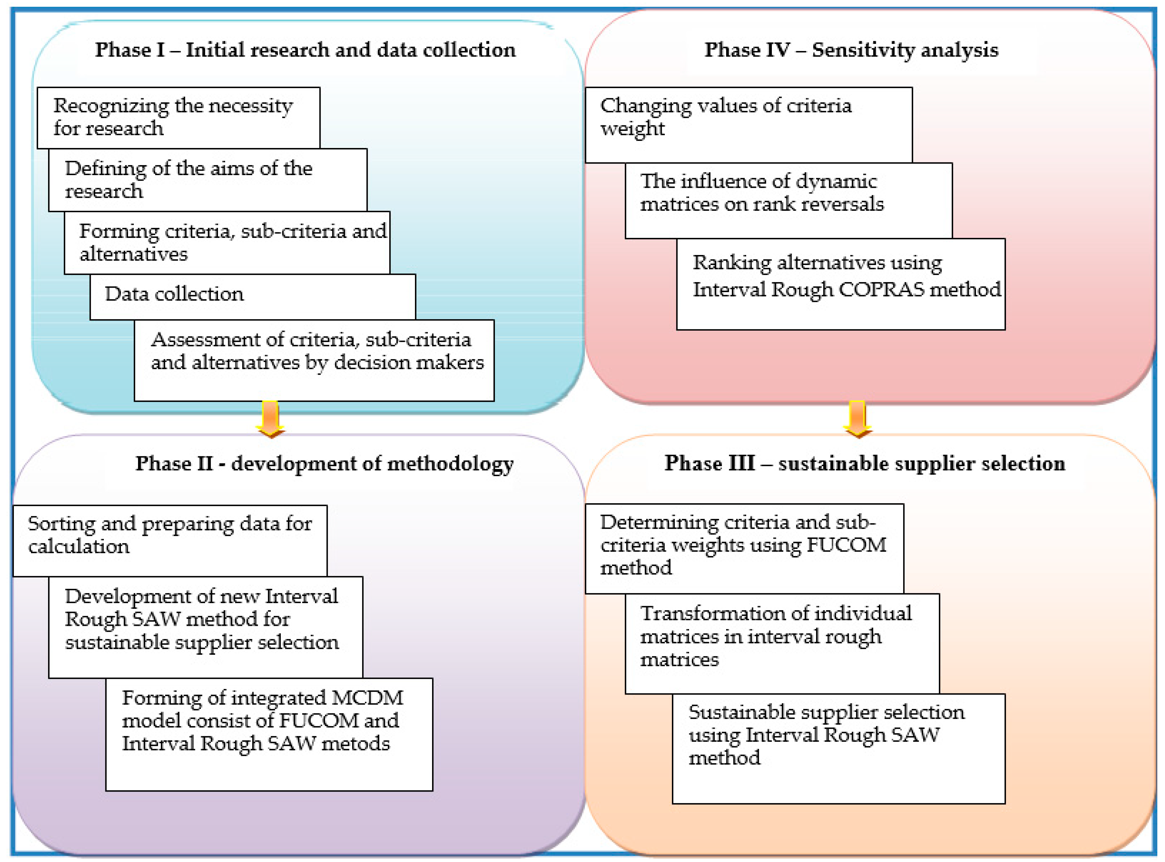
Figure 2.
Algorithms of FUCOM method.
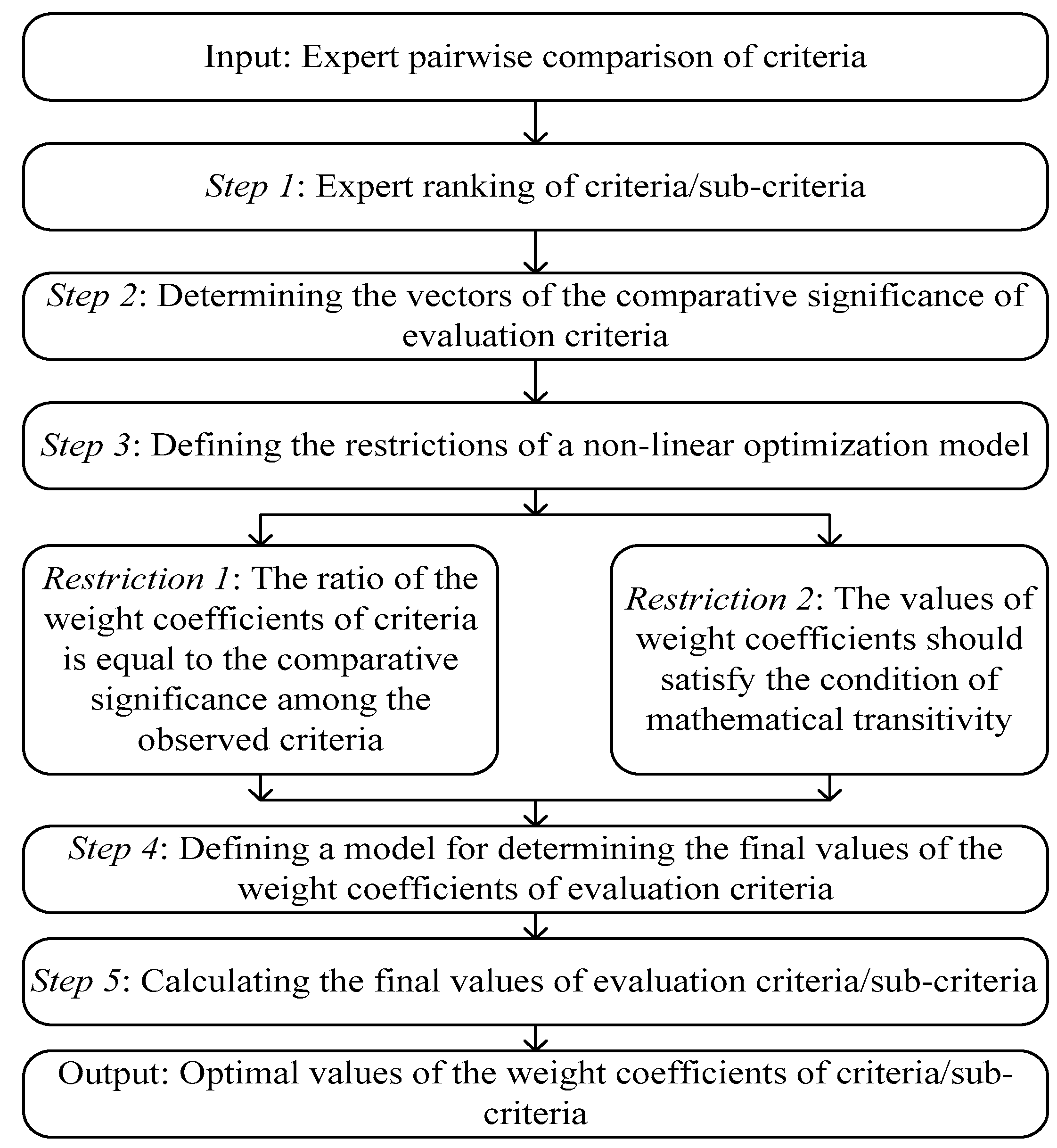
Figure 3.
Criterion evaluation—interval rough and fuzzy evaluation.
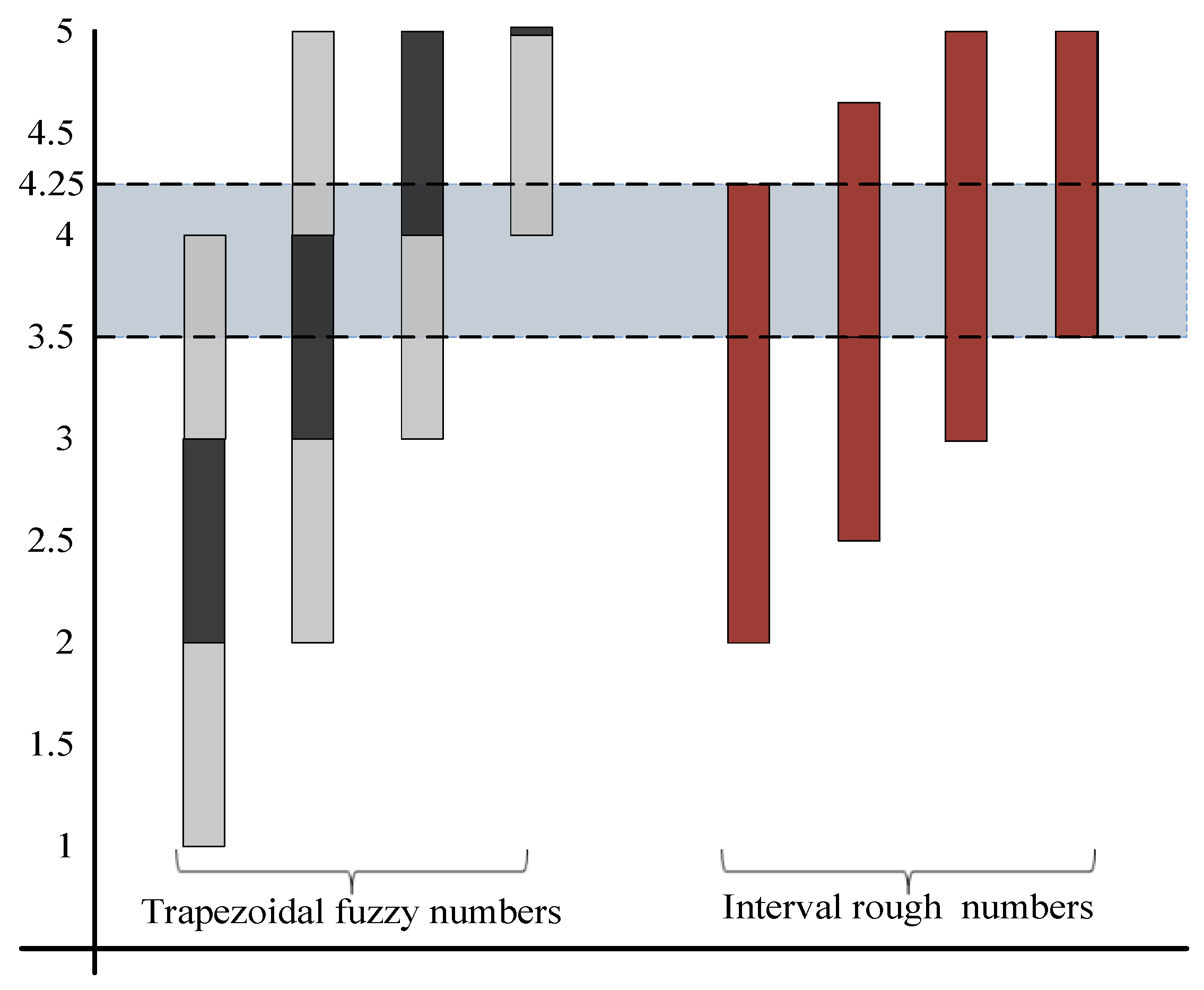
Figure 4.
Ranking interval rough numbers.
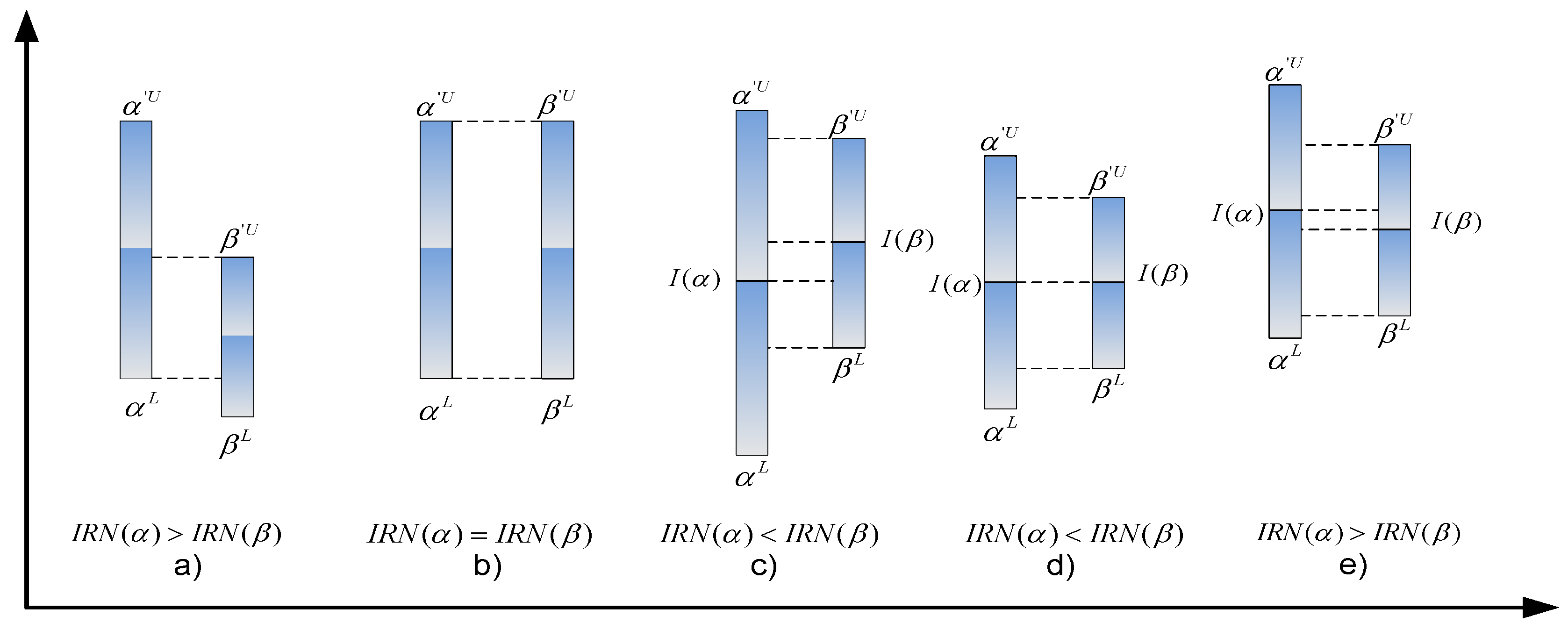
Figure 5.
Sensitivity analysis of alternative rankings across 21 scenarios.

Table 1.
Experts’ evaluation of criterion .
| Criterion | Experts | |||
|---|---|---|---|---|
| E1 | E2 | E3 | E4 | |
| wi | (2;3) | (3;4) | (4;5) | (5;5) |
Table 2.
Evaluation of alternatives by three DMs.
| A1 | A2 | A3 | A4 | |||||||||
|---|---|---|---|---|---|---|---|---|---|---|---|---|
| E1 | E2 | E3 | E1 | E2 | E3 | E1 | E2 | E3 | E1 | E2 | E3 | |
| C11 | (1;1) | (2;3) | (1;2) | (1;2) | (3;4) | (3;3) | (1;2) | (2;2) | (2;2) | (1;2) | (3;3) | (2;3) |
| C12 | (7;8) | (7;7) | (7;8) | (7;7) | (6;7) | (6;7) | (7;8) | (7;7) | (6;7) | (7;7) | (6;7) | (6;7) |
| C13 | (5;6) | (4;5) | (5;6) | (5;6) | (4;5) | (4;5) | (7;8) | (6;7) | (5;5) | (7;7) | (6;7) | (6;6) |
| C14 | (7;7) | (6;7) | (6;7) | (6;6) | (5;6) | (6;6) | (7;7) | (6;7) | (5;5) | (7;7) | (6;6) | (6;7) |
| C15 | (5;5) | (4;5) | (5;5) | (6;7) | (5;6) | (5;5) | (6;6) | (6;7) | (6;6) | (7;8) | (7;7) | (6;6) |
| C16 | (7;8) | (7;8) | (7;8) | (6;7) | (5;6) | (5;6) | (6;7) | (6;6) | (6;6) | (6;7) | (6;6) | (7;8) |
| C17 | (6;6) | (5;6) | (5;5) | (6;6) | (5;5) | (4;5) | (6;7) | (5;6) | (5;6) | (7;7) | (6;7) | (5;6) |
| C21 | (5;6) | (5;5) | (4;5) | (6;6) | (6;7) | (5;6) | (7;7) | (7;7) | (6;6) | (7;8) | (7;7) | (6;6) |
| C22 | (5;5) | (4;5) | (5;5) | (6;6) | (5;5) | (4;4) | (7;8) | (6;7) | (4;5) | (7;7) | (6;6) | (5;6) |
| C23 | (5;6) | (5;5) | (5;6) | (6;7) | (6;7) | (5;5) | (6;7) | (6;7) | (4;5) | (6;6) | (5;6) | (4;5) |
| C24 | (3;4) | (3;3) | (2;3) | (3;4) | (3;3) | (3;4) | (4;4) | (4;5) | (3;3) | (4;5) | (4;4) | (4;4) |
| C25 | (3;4) | (3;4) | (3;4) | (6;6) | (5;5) | (4;5) | (6;6) | (4;5) | (4;4) | (6;7) | (5;6) | (5;6) |
| C26 | (5;5) | (4;5) | (4;5) | (6;6) | (5;6) | (5;6) | (6;6) | (6;7) | (5;5) | (6;6) | (6;7) | (6;6) |
| C27 | (3;3) | (3;3) | (2;2) | (5;6) | (4;5) | (3;4) | (6;7) | (6;6) | (4;4) | (6;7) | (6;6) | (4;5) |
| C31 | (4;5) | (4;4) | (5;6) | (4;4) | (4;5) | (5;5) | (5;6) | (5;6) | (4;5) | (6;6) | (6;6) | (5;6) |
| C32 | (6;6) | (6;6) | (5;6) | (5;6) | (5;5) | (5;6) | (6;7) | (6;7) | (5;6) | (6;6) | (6;6) | (4;5) |
| C33 | (4;4) | (4;4) | (6;6) | (5;5) | (5;6) | (5;6) | (6;6) | (5;5) | (4;4) | (5;6) | (6;6) | (4;5) |
| C34 | (3;4) | (3;3) | (4;4) | (4;4) | (4;5) | (4;4) | (6;6) | (5;5) | (2;3) | (6;6) | (5;5) | (3;4) |
| C35 | (5;6) | (4;5) | (4;5) | (4;4) | (3;4) | (4;4) | (6;6) | (5;5) | (3;4) | (5;5) | (4;5) | (5;5) |
| C36 | (4;4) | (5;5) | (5;5) | (4;5) | (5;5) | (5;5) | (4;5) | (5;5) | (6;6) | (3;4) | (4;4) | (3;4) |
| C37 | (3;4) | (4;4) | (3;4) | (4;5) | (3;4) | (4;4) | (5;5) | (4;5) | (3;4) | (5;5) | (5;6) | (4;4) |
Table 3.
Initial interval rough matrix.
| A1 | A2 | A3 | A4 | |
|---|---|---|---|---|
| C11 | [1.11, 1.55]; [1.5, 2.5] | [1.89, 2.78]; [2.5, 3.5] | [1.45, 1.89]; [2, 2] | [1.5, 2.5]; [2.45, 2.89] |
| C12 | [7, 7]; [7.45, 7.89] | [6.11, 6.55]; [7, 7] | [6.45, 6.89]; [7.11, 7.55] | [6.11, 6.55]; [7, 7] |
| C13 | [4.45, 4.89]; [5.45, 5.89] | [4.11, 4.55]; [5.11, 5.55] | [5.5, 6.5]; [5.89, 7.39] | [6.11, 6.55]; [6.45, 6.89] |
| C14 | [6.11, 6.55]; [7, 7] | [5.45, 5.89]; [5.45, 5.89] | [5.5, 6.5]; [5.89, 6.78] | [6.11, 6.55]; [6.45, 6.89] |
| C15 | [4.45, 4.89]; [5, 5] | [5.11, 5.55]; [5.5, 6.5] | [6, 6]; [6.11, 6.55] | [6.45, 6.89]; [6.5, 7.5] |
| C16 | [7, 7]; [8, 8] | [5.11, 5.55]; [6.11, 6.55] | [6, 6]; [6.11, 6.55] | [6.11, 6.55]; [6.5, 7.5] |
| C17 | [5.11, 5.55]; [5.45, 5.89] | [4.5, 5.5]; [5.11, 5.55] | [5.11, 5.55]; [6.11, 6.55] | [5.5, 6.5]; [6.45, 6.89] |
| C21 | [4.45, 4.89]; [5.11, 5.55] | [5.45, 5.89]; [6.11, 6.55] | [6.45, 6.89]; [6.45, 6.89] | [6.45, 6.89]; [6.5, 7.5] |
| C22 | [4.45, 4.89]; [5, 5] | [4.5, 5.5]; [4.5, 5.5] | [4.89, 6.39]; [5.89, 7.39] | [5.5, 6.5]; [6.11, 6.55] |
| C23 | [5, 5]; [5.45, 5.89] | [5.45, 5.89]; [5.89, 6.78] | [4.89, 5.78]; [5.89, 6.78] | [4.5, 5.5]; [5.45, 5.89] |
| C24 | [2.45, 2.89]; [3.11, 3.55] | [3, 3]; [3.45, 3.89] | [3.45, 3.89]; [3.5, 4.5] | [4, 4]; [4.11, 4.55] |
| C25 | [3, 3]; [4, 4] | [4.5, 5.5]; [5.11, 5.55] | [4.22, 5.11]; [4.5, 5.5] | [5.11, 5.55]; [6.11, 6.55] |
| C26 | [4.11, 4.55]; [5, 5] | [5.11, 5.55]; [6, 6] | [5.45, 5.89]; [5.5, 6.5] | [6, 6]; [6.11, 6.55] |
| C27 | [2.45, 2.89]; [2.45, 2.89] | [3.5, 4.5]; [4.5, 5.5] | [4.89, 5.78]; [4.89, 6.39] | [4.89, 5.78]; [5.5, 6.5] |
| C31 | [4.11, 4.55]; [4.5, 5.5] | [4.11, 4.55]; [4.45, 4.89] | [4.45, 4.89]; [5.45, 5.89] | [5.45, 5.89]; [6, 6] |
| C32 | [5.45, 5.89]; [6, 6] | [5, 5]; [5.45, 5.89] | [5.45, 5.89]; [6.45, 6.89] | [4.89, 5.78]; [5.45, 5.89] |
| C33 | [4.22, 5.11]; [4.22, 5.11] | [5, 5]; [5.45, 5.89] | [4.5, 5.5]; [4.5, 5.5] | [4.5, 5.5]; [5.45, 5.89] |
| C34 | [3.11, 3.55]; [3.45, 3.89] | [4, 4]; [4.11, 4.55] | [3.28, 5.28]; [3.89, 5.39] | [3.89, 5.39]; [4.5, 5.5] |
| C35 | [4.11, 4.55]; [5.11, 5.55] | [3.45, 3.89]; [4, 4] | [3.89, 5.39]; [4.5, 5.5] | [4.45, 4.89]; [5, 5] |
| C36 | [4.45, 4.89]; [4.45, 4.89] | [4.45, 4.89]; [5, 5] | [4.5, 5.5]; [5.11, 5.55] | [3.11, 3.55]; [4, 4] |
| C37 | [3.11, 3.55]; [4, 4] | [3.45, 3.89]; [4.11, 4.55] | [3.5, 4.5]; [4.45, 4.89] | [4.45, 4.89]; [4.5, 5.5] |
Table 4.
Normalized interval rough matrix.
| A1 | A2 | A3 | A4 | |
|---|---|---|---|---|
| C11 | [0.44, 1.03], [0.97, 1.8] | [0.32, 0.62], [0.84, 1.06] | [0.56, 0.78], [0.79, 1.38] | [0.38, 0.63], [0.6, 1.33] |
| C12 | [0.89, 0.94], [1.06, 1.13] | [0.77, 0.88], [1, 1] | [0.82, 0.92], [1.02, 1.08] | [0.77, 0.88], [1, 1] |
| C13 | [0.6, 0.76], [0.83, 0.96] | [0.56, 0.71], [0.78, 0.91] | [0.74, 1.01], [0.9, 1.21] | [0.83, 1.02], [0.98, 1.13] |
| C14 | [0.87, 0.94], [1.07, 1.15] | [0.78, 0.84], [0.83, 0.96] | [0.79, 0.93], [0.9, 1.11] | [0.87, 0.94], [0.98, 1.13] |
| C15 | [0.59, 0.75], [0.73, 0.78] | [0.68, 0.85], [0.8, 1.01] | [0.8, 0.92], [0.89, 1.02] | [0.86, 1.06], [0.94, 1.16] |
| C16 | [0.88, 0.88], [1.14, 1.14] | [0.64, 0.69], [0.87, 0.94] | [0.75, 0.75], [0.87, 0.94] | [0.76, 0.82], [0.93, 1.07] |
| C17 | [0.74, 0.86], [0.84, 1.07] | [0.74, 0.86], [0.79, 1.01] | [0.74, 0.86], [0.94, 1.19] | [0.8, 1.01], [0.99, 1.25] |
| C21 | [0.59, 0.75], [0.74, 0.86] | [0.73, 0.91], [0.89, 1.02] | [0.86, 1.06], [0.94, 1.07] | [0.86, 1.06], [0.94, 1.16] |
| C22 | [0.6, 0.8], [0.77, 0.91] | [0.61, 0.9], [0.69, 1] | [0.66, 1.05], [0.91, 1.34] | [0.74, 1.06], [0.94, 1.19] |
| C23 | [0.74, 0.85], [0.93, 1.08] | [0.8, 1], [1, 1.24] | [0.72, 0.98], [1, 1.24] | [0.66, 0.93], [0.93, 1.08] |
| C24 | [0.54, 0.73], [0.78, 0.89] | [0.66, 0.73], [0.86, 0.97] | [0.76, 0.95], [0.88, 1.13] | [0.88, 0.97], [1.03, 1.14] |
| C25 | [0.46, 0.49], [0.72, 0.78] | [0.69, 0.9], [0.92, 1.09] | [0.64, 0.84], [0.81, 1.08] | [0.78, 0.91], [1.1, 1.28] |
| C26 | [0.63, 0.74], [0.83, 0.83] | [0.78, 0.91], [1, 1] | [0.83, 0.96], [0.92, 1.08] | [0.92, 0.98], [1.02, 1.09] |
| C27 | [0.38, 0.53], [0.42, 0.59] | [0.54, 0.82], [0.78, 1.12] | [0.75, 1.05], [0.85, 1.31] | [0.75, 1.05], [0.95, 1.33] |
| C31 | [0.69, 0.76], [0.76, 1.01] | [0.69, 0.76], [0.76, 0.9] | [0.74, 0.82], [0.93, 1.08] | [0.91, 0.98], [1.02, 1.1] |
| C32 | [0.79, 0.91], [1.02, 1.1] | [0.73, 0.78], [0.93, 1.08] | [0.79, 0.91], [1.1, 1.26] | [0.71, 0.9], [0.93, 1.08] |
| C33 | [0.72, 0.94], [0.77, 1.02] | [0.85, 0.92], [0.99, 1.18] | [0.76, 1.01], [0.82, 1.1] | [0.76, 1.01], [0.99, 1.18] |
| C34 | [0.57, 0.79], [0.64, 0.97] | [0.73, 0.89], [0.76, 1.14] | [0.6, 1.17], [0.72, 1.35] | [0.71, 1.2], [0.83, 1.38] |
| C35 | [0.74, 0.89], [0.95, 1.25] | [0.62, 0.76], [0.74, 0.9] | [0.7, 1.05], [0.83, 1.24] | [0.8, 0.96], [0.93, 1.12] |
| C36 | [0.64, 0.8], [0.82, 0.9] | [0.62, 0.71], [0.82, 0.9] | [0.56, 0.69], [0.73, 0.89] | [0.78, 0.89], [1.13, 1.29] |
| C37 | [0.57, 0.79], [0.82, 0.9] | [0.63, 0.86], [0.84, 1.02] | [0.64, 1], [0.91, 1.1] | [0.81, 1.09], [0.92, 1.24] |
Table 5.
Results of sustainable supplier selection using an integrated FUCOM–interval rough SAW approach.
Table 5.
Results of sustainable supplier selection using an integrated FUCOM–interval rough SAW approach.
| Si | AV | Rank | |||
|---|---|---|---|---|---|
| 0.680 | 0.838 | 0.882 | 1.061 | 0.865 | 3 |
| 0.671 | 0.821 | 0.863 | 1.016 | 0.842 | 4 |
| 0.737 | 0.931 | 0.901 | 1.154 | 0.931 | 2 |
| 0.765 | 0.943 | 0.942 | 1.159 | 0.952 | 1 |
Table 6.
Coefficient of elasticity for changing weights.
| Criteria | Criteria | ||||
|---|---|---|---|---|---|
| C1 | 0.097 | C8 | 0.051 | C15 | 0.034 |
| C2 | 1.000 | C9 | 0.069 | C16 | 0.043 |
| C3 | 0.067 | C10 | 0.036 | C17 | 0.053 |
| C4 | 0.096 | C11 | 0.028 | C18 | 0.031 |
| C5 | 0.064 | C12 | 0.038 | C19 | 0.035 |
| C6 | 0.069 | C13 | 0.046 | C20 | 0.022 |
| C7 | 0.052 | C14 | 0.043 | C21 | 0.027 |
Table 7.
Formed scenarios with new criteria weights.
| Criteria | S1 | S2 | S3 | S4 | S5 | S6 | S7 | S8 | S9 | S10 | S11 | S12 | S13 | S14 | S15 | S16 | S17 | S18 | S19 | S20 | S21 |
|---|---|---|---|---|---|---|---|---|---|---|---|---|---|---|---|---|---|---|---|---|---|
| C1 | 0.0971 | 0.0000 | 0.0671 | 0.0960 | 0.0636 | 0.0694 | 0.0520 | 0.0509 | 0.0694 | 0.0358 | 0.0277 | 0.0382 | 0.0462 | 0.0428 | 0.0335 | 0.0428 | 0.0532 | 0.0312 | 0.0347 | 0.0220 | 0.0266 |
| C2 | 0.0923 | 0.0500 | 0.0637 | 0.0912 | 0.0604 | 0.0659 | 0.0494 | 0.0483 | 0.0659 | 0.0340 | 0.0264 | 0.0362 | 0.0439 | 0.0406 | 0.0318 | 0.0406 | 0.0505 | 0.0297 | 0.0329 | 0.0209 | 0.0253 |
| C3 | 0.0874 | 0.1000 | 0.0603 | 0.0864 | 0.0572 | 0.0624 | 0.0468 | 0.0458 | 0.0624 | 0.0323 | 0.0250 | 0.0343 | 0.0416 | 0.0385 | 0.0302 | 0.0385 | 0.0479 | 0.0281 | 0.0312 | 0.0198 | 0.0239 |
| C4 | 0.0825 | 0.1500 | 0.0570 | 0.0816 | 0.0540 | 0.0590 | 0.0442 | 0.0432 | 0.0590 | 0.0305 | 0.0236 | 0.0324 | 0.0393 | 0.0364 | 0.0285 | 0.0364 | 0.0452 | 0.0265 | 0.0295 | 0.0187 | 0.0226 |
| C5 | 0.0777 | 0.2000 | 0.0536 | 0.0768 | 0.0509 | 0.0555 | 0.0416 | 0.0407 | 0.0555 | 0.0287 | 0.0222 | 0.0305 | 0.0370 | 0.0342 | 0.0268 | 0.0342 | 0.0425 | 0.0250 | 0.0277 | 0.0176 | 0.0213 |
| C6 | 0.0728 | 0.2500 | 0.0503 | 0.0720 | 0.0477 | 0.0520 | 0.0390 | 0.0382 | 0.0520 | 0.0269 | 0.0208 | 0.0286 | 0.0347 | 0.0321 | 0.0251 | 0.0321 | 0.0399 | 0.0234 | 0.0260 | 0.0165 | 0.0199 |
| C7 | 0.0680 | 0.3000 | 0.0469 | 0.0672 | 0.0445 | 0.0486 | 0.0364 | 0.0356 | 0.0486 | 0.0251 | 0.0194 | 0.0267 | 0.0324 | 0.0299 | 0.0235 | 0.0299 | 0.0372 | 0.0218 | 0.0243 | 0.0154 | 0.0186 |
| C8 | 0.0631 | 0.3500 | 0.0436 | 0.0624 | 0.0413 | 0.0451 | 0.0338 | 0.0331 | 0.0451 | 0.0233 | 0.0180 | 0.0248 | 0.0301 | 0.0278 | 0.0218 | 0.0278 | 0.0346 | 0.0203 | 0.0225 | 0.0143 | 0.0173 |
| C9 | 0.0583 | 0.4000 | 0.0402 | 0.0576 | 0.0382 | 0.0416 | 0.0312 | 0.0305 | 0.0416 | 0.0215 | 0.0166 | 0.0229 | 0.0277 | 0.0257 | 0.0201 | 0.0257 | 0.0319 | 0.0187 | 0.0208 | 0.0132 | 0.0160 |
| C10 | 0.0534 | 0.4500 | 0.0369 | 0.0528 | 0.0350 | 0.0382 | 0.0286 | 0.0280 | 0.0382 | 0.0197 | 0.0153 | 0.0210 | 0.0254 | 0.0235 | 0.0184 | 0.0235 | 0.0292 | 0.0172 | 0.0191 | 0.0121 | 0.0146 |
| C11 | 0.0486 | 0.5000 | 0.0335 | 0.0480 | 0.0318 | 0.0347 | 0.0260 | 0.0254 | 0.0347 | 0.0179 | 0.0139 | 0.0191 | 0.0231 | 0.0214 | 0.0168 | 0.0214 | 0.0266 | 0.0156 | 0.0173 | 0.0110 | 0.0133 |
| C12 | 0.0437 | 0.5500 | 0.0302 | 0.0432 | 0.0286 | 0.0312 | 0.0234 | 0.0229 | 0.0312 | 0.0161 | 0.0125 | 0.0172 | 0.0208 | 0.0192 | 0.0151 | 0.0192 | 0.0239 | 0.0140 | 0.0156 | 0.0099 | 0.0120 |
| C13 | 0.0388 | 0.6000 | 0.0268 | 0.0384 | 0.0254 | 0.0277 | 0.0208 | 0.0203 | 0.0277 | 0.0143 | 0.0111 | 0.0153 | 0.0185 | 0.0171 | 0.0134 | 0.0171 | 0.0213 | 0.0125 | 0.0139 | 0.0088 | 0.0106 |
| C14 | 0.0340 | 0.6500 | 0.0235 | 0.0336 | 0.0223 | 0.0243 | 0.0182 | 0.0178 | 0.0243 | 0.0125 | 0.0097 | 0.0134 | 0.0162 | 0.0150 | 0.0117 | 0.0150 | 0.0186 | 0.0109 | 0.0121 | 0.0077 | 0.0093 |
| C15 | 0.0291 | 0.7000 | 0.0201 | 0.0288 | 0.0191 | 0.0208 | 0.0156 | 0.0153 | 0.0208 | 0.0108 | 0.0083 | 0.0114 | 0.0139 | 0.0128 | 0.0101 | 0.0128 | 0.0160 | 0.0094 | 0.0104 | 0.0066 | 0.0080 |
| C16 | 0.0243 | 0.7500 | 0.0168 | 0.0240 | 0.0159 | 0.0173 | 0.0130 | 0.0127 | 0.0173 | 0.0090 | 0.0069 | 0.0095 | 0.0116 | 0.0107 | 0.0084 | 0.0107 | 0.0133 | 0.0078 | 0.0087 | 0.0055 | 0.0066 |
| C17 | 0.0194 | 0.8000 | 0.0134 | 0.0192 | 0.0127 | 0.0139 | 0.0104 | 0.0102 | 0.0139 | 0.0072 | 0.0055 | 0.0076 | 0.0092 | 0.0086 | 0.0067 | 0.0086 | 0.0106 | 0.0062 | 0.0069 | 0.0044 | 0.0053 |
| C18 | 0.0146 | 0.8500 | 0.0101 | 0.0144 | 0.0095 | 0.0104 | 0.0078 | 0.0076 | 0.0104 | 0.0054 | 0.0042 | 0.0057 | 0.0069 | 0.0064 | 0.0050 | 0.0064 | 0.0080 | 0.0047 | 0.0052 | 0.0033 | 0.0040 |
| C19 | 0.0097 | 0.9000 | 0.0067 | 0.0096 | 0.0064 | 0.0069 | 0.0052 | 0.0051 | 0.0069 | 0.0036 | 0.0028 | 0.0038 | 0.0046 | 0.0043 | 0.0034 | 0.0043 | 0.0053 | 0.0031 | 0.0035 | 0.0022 | 0.0027 |
| C20 | 0.0049 | 0.9500 | 0.0034 | 0.0048 | 0.0032 | 0.0035 | 0.0026 | 0.0025 | 0.0035 | 0.0018 | 0.0014 | 0.0019 | 0.0023 | 0.0021 | 0.0017 | 0.0021 | 0.0027 | 0.0016 | 0.0017 | 0.0011 | 0.0013 |
| C21 | 0.0000 | 1.0000 | 0.0000 | 0.0000 | 0.0000 | 0.0000 | 0.0000 | 0.0000 | 0.0000 | 0.0000 | 0.0000 | 0.0000 | 0.0000 | 0.0000 | 0.0000 | 0.0000 | 0.0000 | 0.0000 | 0.0000 | 0.0000 | 0.0000 |
© 2019 by the authors. Licensee MDPI, Basel, Switzerland. This article is an open access article distributed under the terms and conditions of the Creative Commons Attribution (CC BY) license (http://creativecommons.org/licenses/by/4.0/).
Share and Cite
MDPI and ACS Style
Stević, Ž.; Durmić, E.; Gajić, M.; Pamučar, D.; Puška, A. A Novel Multi-Criteria Decision-Making Model: Interval Rough SAW Method for Sustainable Supplier Selection. Information 2019, 10, 292. https://doi.org/10.3390/info10100292
AMA Style
Stević Ž, Durmić E, Gajić M, Pamučar D, Puška A. A Novel Multi-Criteria Decision-Making Model: Interval Rough SAW Method for Sustainable Supplier Selection. Information. 2019; 10(10):292. https://doi.org/10.3390/info10100292
Chicago/Turabian StyleStević, Željko, Elmina Durmić, Mladen Gajić, Dragan Pamučar, and Adis Puška. 2019. "A Novel Multi-Criteria Decision-Making Model: Interval Rough SAW Method for Sustainable Supplier Selection" Information 10, no. 10: 292. https://doi.org/10.3390/info10100292
Note that from the first issue of 2016, this journal uses article numbers instead of page numbers. See further details here.