Blind Queries Applied to JSON Document Stores

Abstract

Social Media, Web Portals and, in general, information systems offer their own Application Programming Interfaces (APIs), used to provide large data sets concerning every aspect of day-by-day life. APIs usually provide data sets as collections of JSON documents. The heterogeneous structure of JSON documents returned by different APIs constitutes a barrier to effectively query and analyze these data sets. The adoption of NoSQL document stores, such as MongoDB, is useful for gathering these data sets, but does not solve the problem of querying the final heterogeneous repository. The aim of this paper is to provide analysts with a tool, named HammerJDB, that allows for blind querying collections of JSON documents within a NoSQL document database. The idea below is that users may know the application domain but it may be that they are not aware of the real structures of the documents stored in the database—the tool for blind querying tries to bridge the gap, by adopting a query rewriting mechanism. This paper is an evolution of a technique for blind querying Open Data portals and of its implementation within the Hammer framework, presented in some previous work. In this paper, we evolve that approach in order to query a NoSQL document database by evolving the Hammer framework into the HammerJDB framework, which is able to work on MongoDB databases. The effectiveness of the new approach is evaluated on a data set (derived from a real-life one), containing job-vacancy ads collected from European job portals.

1. Introduction

Modern portals for publishing advertisements (ads) related to any economical field offer Web Services Application Programming Interfaces (APIs) that allow software systems to publish and retrieve ads. By using the provided API, analysts can easily gather an impressive amount of data for analysis purposes, for example to study the dynamics of social phenomena (possibly) on an international scale.

An interesting application context is offered by the continuously-growing diffusion of Web portals for the labour market (like job portals, employment Web sites and so on); the on-line availability of ads concerning job vacancies enables new research activities for analyzing the labour market and its dynamics [1]. However, web portals for publishing ads are just an example that shows how the Web has become a valuable source of data concerning any aspect of day-by-day life.

Typically, analysts first of all gather the desired data sets to be analyzed, possibly collecting data for a long time; then, they carry on with the analysis itself. The data sets returned by Web services are usually provided as collections of JSON documents. JSON (acronym for JavaScript Object Notation) has become a common syntactic framework that is independent of the specific application context. The consequence is that different Web services provide data sets with different structures, even though they provide the same information (e.g., ads concerning job vacancies). Furthermore, the same source can change the structure of the provided data in time, hence documents gathered from the same source can have different structures because they were gathered in different times. Thus, analysts have to face heterogeneous data structures when they analyze the collected data sets.

Currently, NoSQL Document Stores, able to natively store and query collections of JSON documents, have become very popular, in particular MongoDB (https://www.mongodb.com/) or AWS DocumentDB (https://aws.amazon.com/documentdb/). However, although these systems are schema free by definition, their query languages still lack suitable constructs for flexibly retrieving heterogeneous JSON documents without a precise knowledge of their structure. Consequently, the idea of a fast-search engine developed on top of a JSON document store, able to provide users with a tool that avoids them to explicitly deal with the different structures of the collected data, finds its motivation. The tool we propose is based on a blind-querying approach—users may not be aware of the actual structures of data, but may know the application domain only. The query engine should be able to focus and retrieve the JSON documents of interest. However, at the same time, it should be able to extend the search to those documents that could potentially be of interest, by considering similar field names (both lexically and semantically).

The idea is depicted in Figure 1—several public data sources are collected into a NoSQL JSON-based store. The user tries to retrieve the desired information but finds an insurmountable wall; this is determined by his/her lack of knowledge about the structure of the data contained in the store, as well as by the possibly large variety of different structures of collected data. Blind querying offers an alternative way that allows the user to find relevant information with respect to a simple query. Clearly, we are not considering an operational environment but an analytical environment—one or just a few users every now and then need to query the store to find the desired information.

In this paper, we adapt an approach for blind querying previously developed for querying Open Data Portals [2,3], which creates a catalog describing the meta-data of the data sets published by the open data portals. At query time, users express their queries in a blind way (i.e., irrespective of the actual and heterogeneous structures of data sets). The query can be expressed as a triple including the target data set, the target fields to be retrieved and a selection condition expressed as a Boolean combination of predicates. The query engine expands the user query into a set of queries called, in the sequel, neighbour queries—they are derived by replacing field names in the original user query with similar ones (based both on string similarity and on semantic similarity). The Hammer framework implements the blind querying technique on Open Data portals.

In this paper, we present the HammerJDB framework—it is the first evolution of the Hammer framework towards the application of the blind querying technique to JSON document stores. The current implementation of the HammerJDB framework works on top of MongoDB, but the approach is general and easily adaptable to other JSON document stores. We tested the effectiveness of the approach on a data set concerning the European labour market, extracted and derived from within real-life data downloaded from several online job-vacancy portals to ensure the heterogeneity of the final repository.

The revamping of Hammer (performing queries on Open Data portals) into HammerJDB (for querying JSON document stores) was performed in three main phases:

• Conceptual definition of the problem. In order to move from the context of querying Open Data portals to the context of querying private JSON document stores, the problem has been conceptually reformulated. We studied which previous concepts were still suitable and we defined some new concepts.
• Development of the HammerJDB framework. We developed new connectors to document stores and implemented new concepts, by keeping the core query rewriting technique developed within the former Hammer framework.
• Evaluation. The novel HammerJDB framework has been tested, in order to evaluate its capability to retrieve JSON documents of interest and validate the feasibility of the approach.

The paper is organized as follows. Section 2 discusses the related work, Section 3 presents some introductive notions on NoSQL databases, and Section 4 describes the basic knowledge to understand the presented approach. Section 5 introduces the new approach and some hints about the HammerJDB framework. Section 6 experimentally evaluates performances of the technique for blind querying JSON document stores, by exploiting a data set derived from a corpus of real-life job vacancy ads. Section 7 reports a discussion on some critical aspects, in order to clarify the scope and limitations of the proposed approach. Finally, Section 8 draws conclusions and future work.

2. Related Works

The first definition of blind querying dates back to the birth of the SGML and XMLsemi-structured data formats. When defining query languages for these formats, the problem of querying data collections without a well-defined structure, or with a heterogeneous structure, was soon evident. To tackle this problem, Fuzzy Set Theory [4] was a fairly immediate choice. In References [5,6] an approach based on modeling an XML document as a labeled graph was presented, where a graph is selectively extended by computing fuzzy estimates of the importance of the information it provides, at the granularity of XML tags. The result of such an extension is a fuzzy labeled graph. Query results are sub-graphs of this fuzzy labeled graph, presented as a ranked list according to their degree of matching with respect to the user query. In a different perspective, the approaches presented in References [7,8] propose a flexible XML selection language—named FleXPath—which allows for the formulation of flexible constraints on both structure and content of XML documents. In this way, users can formulate queries that are able to find information that is “close” to the desired one, that is, they formulate blind queries on XML documents.

The task to retrieve relevant information from heterogeneous data sources has several challenges in common with the application domain known as Web Data Extraction. In this domain, software systems are proposed, that automatically and repeatedly extract data from web pages with changing content and delivers the extracted data to a database or some other application ([9]). The common key challenges can be summarized as follows (see Reference [10]):

• Any adopted technique should be able to process large volumes of data in a relatively short time.
• Approaches relying on Machine Learning often require a significantly large training set of manually labeled Web pages or JSON data sets. In general, labeling pages/data sets is a time-expensive and error prone task. As a consequence, in many cases we cannot assume the existence of labeled items.
• Oftentimes, any Web portal extraction tool has to routinely extract data from a source which can evolve over time. Web sources are continuously evolving and structural changes happen with no forewarning, thus are unpredictable. Eventually, in real-world scenarios it emerges the need of maintaining these systems, that might stop working correctly if the are not enough flexible to detect and face the structural modifications of the Web sources they have to interact with.

In different research areas, several query expansion approaches have been proposed, especially in the domain of Information Retrieval, based on user experience. Indeed, with the increasing size of the Web, extracting relevant information by using a query composed just by a few keywords has become a big challenge. Query Expansion (QE) plays a crucial role in improving searches on the Web. In this methodology, the initial query (by the user) is reformulated by adding additional meaningful terms with similar significance. QE—as part of information retrieval (IR)—has long attracted researchers’ attention. It has become very influential in the field of personalized social document, question answering, cross-language IR, information filtering and multimedia IR. Research in QE has gained further prominence because of IR dedicated conferences such as TREC (Text Information Retrieval Conference) and CLEF (Conference and Labs of the Evaluation Forum). A good survey about QE techniques in IR from 1960 to 2017 can be found in Reference [11]. Some interesting works include References [12,13]. Specifically, Reference [12] presents an interactive query expansion model based on a fuzzy association thesaurus for Web information retrieval; Reference [13] proposes a Top-k Query Evaluation with Probabilistic Guarantees.

Focusing on QE techniques based on the analysis of query logs, we can cite Reference [14]. In this work, the authors propose to extract probabilistic correlations among the query terms and the document terms by analyzing the query logs. QE is strictly related to the theme of Total Recall, that is, retrieving all the relevant information with respect to a user query. An interesting paper tackling this issue is Reference [15], where three different extensions to automatic query expansion were proposed:

• a method able to prevent tf-idf failure caused by the presence of sets of correlated features;
• an improved spatial verification and re-ranking step that incrementally builds a statistical model of the query object;
• the concept of relevant spatial context to boost performance of retrieval.

Another interesting paper achieving total recall by means of QE techniques in image retrieval is Reference [16]. In this paper, the authors adopt query expansion for images with two contributions. First, they define some strong spatial constraints between the query image and each result that allow for accurately verifying each return, suppressing the false positives which typically ruin text-based query expansion. Second, the verified images can be used to learn a latent feature model to enable the controlled construction of expanded queries.

In Reference [17], the authors are interested in the growing number of applications that require access to both structured and unstructured data, where the user is totally unaware of the schema of data. These heterogeneous collections of data have been referred to as dataspaces; furthermore, Dataspace Support Platforms (DSSP) are proposed to offer several services over them. One of the key services of a DSSP is seamless querying on the data. The HammerJDB framework can be seen as a DSSP for NoQL JSON document stores, while Reference [17] proposes a DSSP for Web pages.

In Reference [18], the authors report their experience in using Elasticsearch (a distributed full-text search engine) as a solution to manage the heterogeneity of several data sets derived from federated sources. Tools based on the Apache Lucene framework [19], like Elasticsearch and Apache Solr (see Reference [20]), are alternatives to the HammerJDB framework; however, they usually do not retrieve single JSON documents satisfying a selection condition, that is a distinctive feature of HammerJDB.

The core of the Query Engine in the former Hammer framework was implemented by using the Map-Reduce paradigm [21]. The Query Engine of the new HammerJDB framework has inherited the query-engine core, thus it is a Map-Reduce algorithm too.

The benefits of the Map-Reduce approach are described in Reference [22]. Map-Reduce has been highly successful in implementing large-scale data-intensive applications on commodity clusters.

In few words, Map-Reduce frameworks automatically parallelize and execute the program on a (possibly large) cluster of computers. In Reference [23], the authors present YARN (acronym for Yet Another Resource Negotiator) and they provide experimental evidence demonstrating the improvements of using YARN on production environments. YARN is the basic component within the very popular Hadoop framework, responsible for handling the actual execution of the Map-Reduce jobs.

In Reference [24], the researchers present the Spark framework, a popular alternative to Hadoop as a Map-Reduce framework. In order to efficiently support data-transforming applications, Spark introduces an abstraction called Resilient Distributed Dataset (RDDs). An RDD is a main-memory and read-only collection of data partitioned across a set of machines that can be rebuilt if a partition is lost. Spark is still a Map-Reduce framework, where Map-Reduce programming can be explicit or implicit. In Reference [25], we presented various implementation of the former Hammer framework for querying Open Data portals, that adopt both Hadoop and Spark; the results show that Spark can be very efficient, in particular if its high-level programming abstractions are exploited. Thus, since the Spark version demonstrated to be the most efficient one, the novel HammerJDB framework is based on the Spark version of the query-engine core. Hammer and HammerJDB are implemented on top of MongoDB, but they use it only as a pure storage technology and do not rely on its internal query language and (consequently) on the Map-Reduce support provided by it; this choice allows us to be independent of specific execution platforms and storage technology during the development; for example, we moved form the original Hadoop-based implementation to the current Spark-based implementation, seamlessly with respect to the storage technology; furthermore, the scalability of the approach (see Reference [25]) is guaranteed independently of the storage technology.

3. Basic Concepts on NoSQL Databases for JSON Documents

In this section, we introduce some general concepts concerning the world of NoSQL databases for JSON documents. These systems constitute a specific class of NoSQL databases, that is, databases that do not rely on the relational data model and (consequently) cannot be queried by means of the SQL query language. The interested reader can refer to Reference [26] for a recent survey on the current scenario concerning NoSQL databases.

Within this wide family of systems, we consider NoSQL databases for JSON documents, that is, databases able to store JSON documents in a native way. These systems are also called document databases or JSON document stores.

For completeness, we briefly introduce some basic concepts concerning JSON and document databases.

3.1. JSON Documents

JSON is the acronym for JavaScript Object Notation—it was born as a textual format to represent and define objects within the JavaScript programming language. The interested reader can find the specification in Reference [27]. The process to obtain the JSON version of a main memory JavaScript object is called serialization, while the process to obtain a main memory JavaScript object from a JSON representation is called deserialization. Since JSON is often used to interchange data concerning documents, JSON data are also called documents (even thought they derive from main memory objects).

In the following, we informally introduce the JSON format, by means of the excerpt reported in Listing 1.

• A JSON document is enclosed within a pair of braces { and }, that encompasses a list of comma-separated fields.
• Syntactically, a field is a name: value pair, where the name is a string contained within a pair of " characters.
• The value of a field can alternatively be:

  -

  A constant (possibly negative) integer or real number;

  -

  a constant string, enclosed either within a pair of " characters;

  -

  a nested document, enclosed within { and }, arbitrarily complex;

  -

  an array of values, uncolored within characters [ and ], where an item can be either a numerical value or a string value or a document or an array.

Listing 1. Excerpt of JSON document.

{

‘‘a’’: 1,

‘‘b’’: {

‘‘c n’’: ‘‘c1’’,

‘‘d’’: ‘‘d1’’

},

‘‘f’’: { ‘‘f1’’: {

‘‘c n’’: ‘‘c2’’,

‘‘d’’: ‘‘d2’’

},

‘‘f2’’: {

‘‘c n’’: ‘‘c3’’,

‘‘d’’: ‘‘d3’’

}

}

}

Listing 1. Excerpt of JSON document.

{

‘‘a’’: 1,

‘‘b’’: {

‘‘c n’’: ‘‘c1’’,

‘‘d’’: ‘‘d1’’

},

‘‘f’’: { ‘‘f1’’: {

‘‘c n’’: ‘‘c2’’,

‘‘d’’: ‘‘d2’’

},

‘‘f2’’: {

‘‘c n’’: ‘‘c3’’,

‘‘d’’: ‘‘d3’’

}

}

}

Although fields may be arrays (as reported above), it is quite difficult to express blind queries on them. For this reason, we decided to consider only documents without arrays, by relying on the consideration that documents containing arrays can be simplified by applying an unnest() function able to expand a document containing an array to a set of documents, one for each item in the original array. However, this solution may cause the combinatorial explosion of unnested documents, in particular in case of documents containing multiple (possibly nested) arrays. An alternative way is to unroll arrays: an array with name a, containing n items,, is replaced by n fields with name a_i (with $1\le i\le n$), where the value of each a_i field is the item in position i in the original array.

As an example, consider the sample JSON document reported in Listing 1. At the upper level, it is composed of three fields, named “a”, “b” and “f”, respectively. Specifically, the “a” field has an integer numerical value, while the value of the “b” field is a nested document and the value of the “f” field is a nested document containing, in turns, two nested documents.

Looking at the “b” field, it is a document composed of two string-valued fields. Notice that the name of the “c n” field contains a blank character.

Finally, notice that the value of the “f” field: it is a nested document having two fields, named “f1” and “f2”, that in turn are further nested documents.

In order to reason about the structure of JSON documents, we introduce the concept of field path.

Definition 1.

Field Path Given a JSON document d, we denote a field within d by means of its path, that is, a dot notation with syntax|(.name$)+$|, where name is a field name; the first dot denotes that the first field is rooted in the upper level of the document; then, a path with more than one name refers to a nested field.

As an example, consider the sample JSON object reported in Listing 1. The path |.“a”| refers to a rooted field named “a”. The path |.“b”.“d”| refers to a field named “d” that is contained within the field named “b”. The path expression |.“f”.“f1”.“c n”| refers to the “c n” field of the second-level nested document named “f1”, within field “f”.

In our approach, paths are expressed by using the dot notation, following the J-CO-QL transformation language for collections of JSON documents presented in [28,29,30,31].

3.2. Document Databases

We can now present the basic definitions that characterize NoSQL databases for JSON documents. We rely on the terminology provided by MongoDB, but this terminology is common in this context.

Definition 2.

Collection. A collection $c=\{d_1,d_2,\dots ,\}$ is a heterogeneous set of JSON documents $d_i$, without any constraint on the structure of these documents.

Thus, a collection plays the same role as tables in relational databases. However, a collection can contain any kind of document—in principle, each document in the collection may be structurally different from the other documents in the same collection.

Definition 3.

Database Model. A database is a set $db=\{c_1,c_2,\dots \}$ of collections. Each collection is identified by a unique name within the database.

Example 1.

Suppose we are collecting job-vacancy ads from portals of several European countries. Though the semantic content of each ad is, at the end, the same, and even though they are all represented as JSON documents, their structure is not the same.

Thus, we could organize the database as two collections of ads—the first one, named SouthernCountriesAds, collects ads concerning countries in southern Europe, and a sample instance is reported in Listing 2; the second collection, named NorthernCountriesAds, collects ads concerning countries in northern Europe, and a sample instance is reported in Listing 3.

Listing 2. Sample collection SoutherCountriesAds.

{ ‘‘ID’’: 1,

‘‘Offer’’: { ‘‘Title’’: ‘‘Finance Manager ’’,

‘‘Description’’: ‘‘Department’s finances’’,

‘‘Country’’: ‘‘IT’’,

‘‘Salary’’: ‘‘To be defined’’ },

‘‘Publish date’’: ‘‘03/09/2018’’ }

{ ‘‘ID’’: 2,

‘‘Profession’’: ‘‘International Export/Sales Manager’’,

‘‘Profile’’: ‘‘An International Export / Sales Manager’’,

‘‘Place’’: { ‘‘Location’’: ‘‘Valencia’’,

‘‘Country’’: ‘‘Spain’’ },

‘‘Release date’’: ‘‘13/09/2018’’ }

{ ‘‘ID’’: 3,

‘‘Profession’’: ‘‘Solution Services Marketing Manager ’’,

‘‘Profile’’: ‘‘8--10 years of experience in Marketing.’’,

‘‘Place’’: { ‘‘Location’’: ‘‘Barcelona’’,

‘‘Country’’: ‘‘Spain’’ },

‘‘Release date’’: ‘‘17/09/2018’’ }

Listing 2. Sample collection SoutherCountriesAds.

{ ‘‘ID’’: 1,

‘‘Offer’’: { ‘‘Title’’: ‘‘Finance Manager ’’,

‘‘Description’’: ‘‘Department’s finances’’,

‘‘Country’’: ‘‘IT’’,

‘‘Salary’’: ‘‘To be defined’’ },

‘‘Publish date’’: ‘‘03/09/2018’’ }

{ ‘‘ID’’: 2,

‘‘Profession’’: ‘‘International Export/Sales Manager’’,

‘‘Profile’’: ‘‘An International Export / Sales Manager’’,

‘‘Place’’: { ‘‘Location’’: ‘‘Valencia’’,

‘‘Country’’: ‘‘Spain’’ },

‘‘Release date’’: ‘‘13/09/2018’’ }

{ ‘‘ID’’: 3,

‘‘Profession’’: ‘‘Solution Services Marketing Manager ’’,

‘‘Profile’’: ‘‘8--10 years of experience in Marketing.’’,

‘‘Place’’: { ‘‘Location’’: ‘‘Barcelona’’,

‘‘Country’’: ‘‘Spain’’ },

‘‘Release date’’: ‘‘17/09/2018’’ }

Listing 3. Sample collection NorthernCountriesAds.

{ ‘‘ID’’: 1,

‘‘Job Title’’: ‘‘Junior project controller’’,

‘‘Area’’: { ‘‘City’’: ‘‘Berlin’’,

‘‘Country’’: ‘‘DE’’ },

‘‘Offer’’: { ‘‘Contract’’: ‘‘Permanent’’,

‘‘Working Hours’’: ‘‘Full Time’’},

‘‘Release date’’: ‘‘19/09/2018’’ }

{ ‘‘ID’’: 2,

‘‘Offer’’: { ‘‘Job Title’’: ‘‘Supplier Engineer’’,

‘‘Place’’: { ‘‘City’’: ‘‘Berlin’’,

‘‘Country’’: ‘‘DE’’ } },

‘‘Release date’’: ‘‘17/09/2018’’

}

Listing 3. Sample collection NorthernCountriesAds.

{ ‘‘ID’’: 1,

‘‘Job Title’’: ‘‘Junior project controller’’,

‘‘Area’’: { ‘‘City’’: ‘‘Berlin’’,

‘‘Country’’: ‘‘DE’’ },

‘‘Offer’’: { ‘‘Contract’’: ‘‘Permanent’’,

‘‘Working Hours’’: ‘‘Full Time’’},

‘‘Release date’’: ‘‘19/09/2018’’ }

{ ‘‘ID’’: 2,

‘‘Offer’’: { ‘‘Job Title’’: ‘‘Supplier Engineer’’,

‘‘Place’’: { ‘‘City’’: ‘‘Berlin’’,

‘‘Country’’: ‘‘DE’’ } },

‘‘Release date’’: ‘‘17/09/2018’’

}

4. Blind Querying on Open Data: Definitions and Approach

In this section, we briefly present Hammer, the framework for blind querying Open Data. This framework constitutes the background of the present work—it was introduced in Reference [2] and further improved in in Reference [3]; in this paper, we rely on the latter version [3].

The blind querying approach was adopted for retrieving data sets of interest published by Open Data portals. Since these corpora usually contain a large number of data sets, it is not possible to know their structure in advance. Thus, we developed a framework for blind querying: the user formulates a query that has to be translated by the query engine to the actual structure of data sets within the corpus. In this section, we review some basic concepts and definitions (Section 4.1) and briefly describe the blind querying approach (Section 4.2).

4.1. Basic Concepts and Definitions

An Open Data portal is an access point to open data published by institutions, agencies and other bodies. It is possible to use and re-use this information for either commercial or non-commercial purposes. As a consequence, a portal offers a corpus of data sets; the blind querying approach aims at querying these data sets, in order to get those data items (documents) relevant with respect to the query. Hereafter, we report the most important definitions.

Definition 4.

(Flat) Data Set. A Data Set is a collection of data items, where each item may be a flat record or a row or a tuple, that is, without nested structures. All data items in a Data Set share the same schema (field names and data types).

A Data Set ds is represented by an internal identifier id, a name and an Instance (set of data items belonging to the Data Set), respectively denoted as $ds.id$, $ds.name$ and $Instance\left(ds\right)$.

Definition 5.

Corpus and Catalog. Let C = {$d{s}_1$, $d{s}_2$, ⋯} be the Corpus of Data Sets. The Catalog of the corpus is the list of descriptions $descr\left(d{s}_i\right)=\langle fields,metadata\rangle$ (with $d{s}_i\in C$), where $fields$ is a set of pairs denoting a field name and its data type, while $metadata$ is a set of key-value pairs, associating a key meta-data item with its value (often, metadata items are provided by Open Data portals).

Let’s now give the definition of Query.

Definition 6.

Query. (From [3]) Given a Data Set Name $dn$, a set P of field names (properties) of interest $P=\{p{n}_1,p{n}_2,\dots \}$ and a selection condition $sc$ on field values, a query q is a triple $q:\langle dn,P,sc\rangle$.

Notice that a selection condition is a Boolean composition of predicates between fields and their values; predicates can be composed by means of the classical AND, OR and NOT operators, as well as by means of parentheses ( and ), to express complex conditions. Field values are numerical or string constants.

Furthermore, data set names and field (property) names can contain more than one word, possibly separated by blanks, underscores, lines, and so on (for example, “City Name”). For this reason, they are enclosed within characters [ and ].

Finally, field names are also called field-name terms.

Definition 7.

Query Term. (From [3]) With Query Term (term for simplicity) we denote either a Data Set Name $q.dn$ or a Field Name Term appearing either in $q.P$ or in $q.sc$ or both, as well as a Constant appearing in $q.sc$.

Example 2.

As an example, suppose that a labour market analyst may be interested to get information about job offers for a “Software Developer” located in a given city named “My City.” The query may be written as:

• $q:\langle dn=$[Job-Offers],
• P $=\{$[Company], [Requirements], [Contract] },
• sc $=($[City]=“My City” AND [Profession]=“Software Developer”$)\rangle$.

Notice that data set name and field names are enclosed within characters [ and ], in order to allow users to specify names with blanks.

Definition 8.

Neighbour Query. Consider a query $q:\langle dn,P,sc\rangle$, and its list of terms $T\left(q\right)$. Consider a substitution function $sf:T\left(q\right)\to T^{\prime }\left(q\right)$, that generates a list $T^{\prime }\left(q\right)$ of terms ($\left|T\left(q\right)\right|=|T^{\prime }\left(q\right)|$) such that for each pair $t_i\in T\left(q\right)$ and $t_i^{\prime }\in T^{\prime }\left(q\right)$ of corresponding terms, it can be either $t_i=t_i^{\prime }$ (no substitution) or $t_i\ne t_i^{\prime }$ (substitution).

The Neighbour Query $nnq:\langle dn,P,sc\rangle$ is obtained from q by performing the substitution denoted by $T\left(q\right)$ and $T^{\prime }\left(q\right)$, that is, $nq.ds$, $nq.P$ and $nq.sc$ are obtained from $q.dn$, $q.P$ and $q.sc$ (respectively) by replacing each term t with $sf\left(t\right)$.

The role of the substitution function $sf$ is thus critical. In our approach, we consider both lexical similarity (based on the Jaro-Winkler similarity measure [32]) and semantic similarity (based on the WordNet dictionary [33]). Details are reported in Reference [3].

Example 3.

Consider again the query q in Example 2. In the corpus C, there may not exist a data set with name Job-Offers, as well as the desired job vacancies may be in a different data set named Jobs. So, the data items of interest may be retrieved by a slightly different query, that is,

• $n{q}_1:\langle dn=$[Jobs],
• $P=\{$[Company], [Requirements], [Contract]},
• $sc=($[City]=“My City” AND [Profession]=“Software Developer”$)\rangle$.

The query $n{q}_1$ is obtained by rewriting query q: the data set name $q.dn=$ [Job-Offers] is replaced by [Jobs]. As the reader may notice, the rewritten query contains $n{q}_1.dn=$ [Jobs].

Another possible rewritten query may be obtained by replacing the property [City] with [Job-Location]. In this case, we obtain the following rewritten query $n{q}_2$.

• $n{q}_2:\langle dn=$[Job-Offers],
• $P=\{$[Company], [Requirements], [Contract]},
• $sc=($[Job-Location]=“My City” AND [Profession]=“Software Developer”$)\rangle$

Furthermore, another rewritten query $n{q}_3$ may be obtained by substituting two terms.

• $n{q}_3:\langle dn=$[Jobs],
• $P=\{$[Company], [Requirements], [Contract]},
• $sc=($[Job-Location]=“My City” AND [Profession]=“Software Developer”$)\rangle$

Query $n{q}_3$ searches for a data set named [Jobs] and selects the items that contain the [Job-Location] field with value “My City”.

Queries $n{q}_1$, $n{q}_2$ and $n{q}_3$ constitute the neighbourhood of q; for this reason, they are called Neighbour Queries.

We can now formulate the problem that the Hammer framework has to solve.

Problem 1.

Given a corpus C of data sets, the execution of a query q returns the result set $RS=\{d_1,d_2,\dots \}$, that contains the data items $d_i$ retrieved in the data sets $d{s}_j\in C$ ($d_i\in Instance\left(d{s}_j\right)$) such that $d_i$ satisfies the query q or a neighbour query $nq$ obtained by rewriting the query q.

4.2. Hammer, the Blind Querying Framework

Hammer is the framework developed for blind querying Open Data portals, fully explained in [25] and briefly summarized in this section.

The Hammer framework consists of two main components: the Indexer (Section 4.2.1) and the Query Engine (Section 4.2.2). Figure 2 depicts the application scenario.

4.2.1. Indexer

The Hammer framework was designed to query data sets published on an Open Data portal. The first requirement was to obtain descriptions concerning the data sets without downloading their (possibly huge) instances; in this way, the download of the data set instances is delayed to query time.

Thus, the Indexer (see Figure 2), performs several activities described in the following.

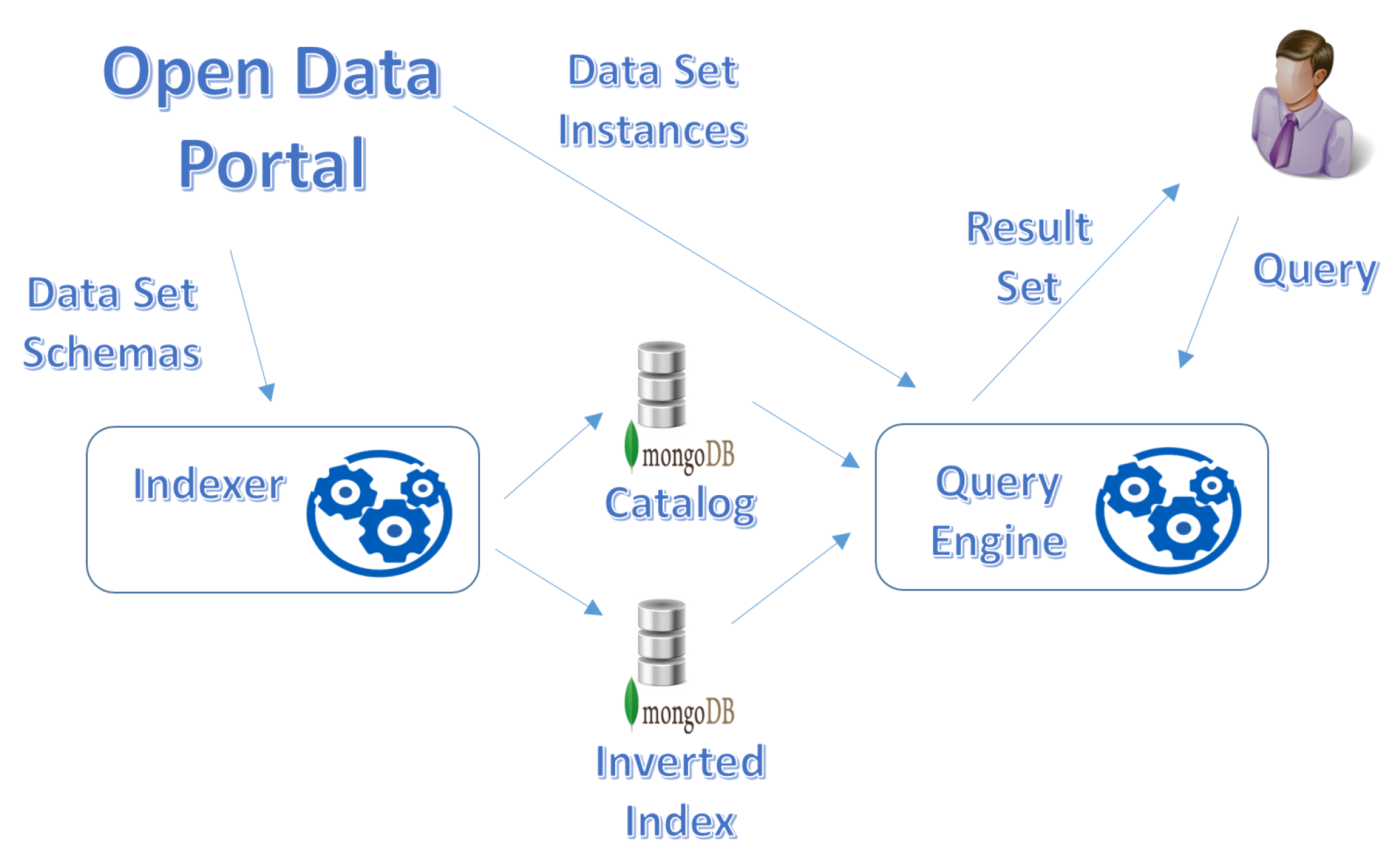
• Crawling. the Indexer crawls the Open Data portal, in order to gather the list of published data sets, and for each of them its schema and auxiliary meta-data are extracted.
• The data set descriptions are stored into the catalog of the corpus; among several choices, we employed MongoDB to store the catalog, for the sake of flexibility.
• Indexing. The schema and the meta-data of the gathered data sets are indexed by means of an Inverted Index, a key-value data structure where the key is a term appearing in the data set descriptor (typically, the data set name and the field names), while the value is a list of data set identifiers (see Definition 4) that are associated with the term. Again, for the sake of flexibility, we adopted MongoDB to store the inverted index too.

The Indexer pre-processes data sets published by the Open Data portal, in order to enable the blind querying process.

4.2.2. Query Engine

The user wishing to query the corpus submits a query q to the Query Engine (see Figure 2) to retrieve the relevant items. Here, we summarize how the query is evaluated.

• Step 1: Term Extraction and Retrieval of Alternative Terms. The set $T\left(q\right)$ of terms is extracted from within $q.dn$, $q.P$ and $q.sc$. Then, for each term $t\in T\left(q\right)$, the set $Alt\left(t\right)$ of similar terms is built. A term $t^{\prime }\in Alt\left(t\right)$ if $t^{\prime }$ is present in the catalog and either if it is lexicographically similar (based on the Jaro-Winkler similarity measure) or semantically similar (synonym) based on WordNet dictionary, or a combination of both.
• Step 2: Neighbour Queries. For each term $t\in T\left(q\right)$, the alternative terms $Alt\left(t\right)$ are used to compute, from the original query q, the Neighbour Queries (see Definition 8) The set $Q=\{q{p}_1,q{p}_2,\dots \}$ of queries to process contains both q and the derived neighbour queries.
• Step 3: VSM Data Set Retrieval. For each query $qp\in Q$, the set of terms $T\left(qp\right)$ is used to retrieve the data sets, represented by means of the Vector Space Model [34]. The cosine similarity is computed as relevance measure of a data set with respect to terms in the query $qp$; the relevance measure is denoted as $krm(ds,qp)\in [0,1]$; only data sets with $krm(ds,qp)\ge th\_krm$ (where $th\_krm$ is a pre-defined minimum threshold) are selected for next steps. The Inverted Index (Figure 2) is essential to efficiently select data sets by computing $krm(ds,qp)$. The set of extracted data sets is denoted as $DS$.
  To sum up, this step extracts the data sets that own the largest number of terms in common with the query, because the greater the number of the common terms, the higher the relevance of the data set with respect to the query.
• Step 4: Schema Fitting. In this step, a comparison between the set of field names in each query $qp\in Q$ and the schema of each selected data set in $DS$ is performed, in order to compute the Schema Fitting Degree $sfd(ds,qp)\in [0,1]$ (see [3] for its definition): the data set whose schema better fits the list $T\left(qp\right)$ of terms in query $qp$ is the most relevant (higher $sfd(ds,qp)$) with respect to the other data sets; for example, if some field appearing in the selection condition is missing in the data set, the query cannot be executed.
  The overall relevance measure $rm(ds,qp)$ of a data set $ds$ with respect to a query $qp$ is obtained as a linear combination of the keyword relevance measure $krm(ds,qp)$ and the schema fitting degree $sfd(ds,qp)$:

  $$rm(ds,qp)=\alpha \times krm(ds,qp)+(1-\alpha )\times sfd(ds,qp)$$

  (1)
  This step returns the set of result data sets $RDS$: a data set $ds\in RDS$ if its global relevance measure is greater than or equal to a minimum threshold $th\_rm$, that is, $rm(ds,qp)\ge th\_rm$ for at least one query $qp\in Q$.
• Step 5: Instance Filtering. The Query Engine retrieves and downloads the instances of the data sets returned by Step 4 (see Figure 2) in $RDS$. The queries $qp\in Q$ are evaluated on the downloaded instances, in order to find out those data items that satisfy at least one query $qp$. These data items constitute the result set $RS$ produced by the Query Engine and provided to the user (see Problem 1).

To run the query process, three minimum thresholds must be set: the first one is the minimum string similarity threshold th_sim $\in [0,1]$, which is used in Step 1 to select only terms lexicographically very similar to original terms; the minimum threshold th_krm $\in [0,1]$ for cosine similarity of data sets with respect to queries in Q; the minimum relevance threshold th_rm$\in [0,1]$ for data sets. Furthermore, the $\alpha$ factor in Equation (1) must be set too.

5. Blind Querying on NoSQL Databases for JSON Documents

In this section, we present the HammerJDB framework: it is the evolution of the Hammer framework (shortly presented in Section 4), towards blind querying NoSQL databases of JSON documents (see Section 3). This is the novel contribution of the paper.

Figure 3 depicts the scenario, where the two components that constitute the HammerJDB framework are reported. In the following, we first introduce some new concepts; then, we discuss both the Indexer and the Query engine of the HammerJDB framework.

5.1. Novel Concepts

In Section 3, we introduced the basic concepts concerning JSON and NoSQL databases for JSON documents. Now, we need to define fields and documents.

Definition 9.

Field Descriptor. Given a JSON document d and a Field f (in d) denoted by its Path p (see Definition 1), the Field Descriptor $fd=\langle p,n,t\rangle$ is a triple including the path p, the field name n and the (data) type t.

Specifically, we consider the following (data) types $t=$ “string” (for string-valued fields), $t=$ “number” (for numerical fields) and $t=$ “document” (for nested documents).

The notion of field descriptor is necessary to define the concept of Document Schema.

Definition 10.

Document Schema. Given a JSON document d, its Schema is defined as

$$Schema\left(d\right)=\{f{d}_1.\dots \}$$

where descriptors $f{d}_i$ describe all and only all elementary fields (with type $t=$ “string” or $t=$ “number”).

By relying on the previous definitions, we can handle the heterogeneity that characterizes collections within the database (see Section 3.2). In fact, Definition 4, designed for Open Data sets, is no longer suitable. We provide a new interpretation of the concept of Data Set.

Definition 11.

JSON Data Set and Corpus. A JSON Data Set $jds$ is a set of homogeneous JSON documents, that is, having the same schema, stored within the same database collection. A JSON data set is described by a tuple

$$jds:\langle ds\_id,collection\_name,schema\rangle$$

where $ds\_id$ is a unique identifier, $collection\_name$ is the name of the collection (not unique) which the JSON data set is extracted from; $schema$ is the structure representation of documents in the JSON data set (as defined by Definition 10).

The instance of the JSON data set, denoted as $Instance\left(jds\right)$, is the set of homogeneous documents aggregated within the JSON data set.

The set of JSON data sets extracted from collections in the database is denoted as $JC$, that is the Corpus of JSON data sets.

Listing 4. JSON data sets from the SoutherCountriesAds collection (reported in Listing 2).

JSON Data Set

$\langle ds\_id=$1,

collection_name=“SouthernCountriesAds”,

schema$=\{\langle$|.“ID”|, “ID”, “number”〉,

〈|.“Offer”.“Title”|, “Title”, “String”〉,

〈|.“Offer”.“Description”|, “Description”, “String”〉,

〈|.“Offer”.“Country”|, “Country”, “String”〉,

〈|.“Offer”.“Salary”|, “Salary”, “String”〉,

〈|.“Publish date”|, “Publish Date”, “String”$\rangle \}\rangle$

Instance

{ ‘‘ID’’: 1,

‘‘Offer’’: { ‘‘Title’’: ‘‘Finance Manager ’’,

‘‘Description’’: ‘‘Department’s finances’’,

‘‘Country’’: ‘‘IT’’,

‘‘Salary’’: ‘‘To be defined’’ },

‘‘Publish date’’: ‘‘03/09/2018’’ }

JSON Data Set

$\langle ds\_id=$2,

collection_name=“SouthernCountriesAds”,

schema$=\{\langle$|.“ID|”, “ID”, “number”〉,

〈|.“Profession”|, “Profession”, “String”〉,

〈|.“Profile”|, “Profile”, “String”〉,

〈|.“Place”.“Location”|, “Location”, “String”〉,

〈|.“Place”.“Country”|, “Country”, “String”〉,

〈|.“Release date”|, “Release Date”, “String”$\rangle \}\rangle$

Instance

{ ‘‘ID’’: 2,

‘‘Profession’’: ‘‘International Export/Sales Manager’’,

‘‘Profile’’: ‘‘An International Export / Sales Manager’’,

‘‘Place’’: { ‘‘Location’’: ‘‘Valencia’’,

‘‘Country’’: ‘‘Spain’’ },

‘‘Release date’’: ‘‘13/09/2018’’ }

{ ‘‘ID’’: 3,

‘‘Profession’’: ‘‘Solution Services Marketing Manager ’’,

‘‘Profile’’: ‘‘8--10 years of experience in Marketing.’’,

‘‘Place’’: { ‘‘Location’’: ‘‘Barcelona’’,

‘‘Country’’: ‘‘Spain’’ },

‘‘Release date’’: ‘‘17/09/2018’’ }

Listing 4. JSON data sets from the SoutherCountriesAds collection (reported in Listing 2).

JSON Data Set

$\langle ds\_id=$1,

collection_name=“SouthernCountriesAds”,

schema$=\{\langle$|.“ID”|, “ID”, “number”〉,

〈|.“Offer”.“Title”|, “Title”, “String”〉,

〈|.“Offer”.“Description”|, “Description”, “String”〉,

〈|.“Offer”.“Country”|, “Country”, “String”〉,

〈|.“Offer”.“Salary”|, “Salary”, “String”〉,

〈|.“Publish date”|, “Publish Date”, “String”$\rangle \}\rangle$

Instance

{ ‘‘ID’’: 1,

‘‘Offer’’: { ‘‘Title’’: ‘‘Finance Manager ’’,

‘‘Description’’: ‘‘Department’s finances’’,

‘‘Country’’: ‘‘IT’’,

‘‘Salary’’: ‘‘To be defined’’ },

‘‘Publish date’’: ‘‘03/09/2018’’ }

JSON Data Set

$\langle ds\_id=$2,

collection_name=“SouthernCountriesAds”,

schema$=\{\langle$|.“ID|”, “ID”, “number”〉,

〈|.“Profession”|, “Profession”, “String”〉,

〈|.“Profile”|, “Profile”, “String”〉,

〈|.“Place”.“Location”|, “Location”, “String”〉,

〈|.“Place”.“Country”|, “Country”, “String”〉,

〈|.“Release date”|, “Release Date”, “String”$\rangle \}\rangle$

Instance

{ ‘‘ID’’: 2,

‘‘Profession’’: ‘‘International Export/Sales Manager’’,

‘‘Profile’’: ‘‘An International Export / Sales Manager’’,

‘‘Place’’: { ‘‘Location’’: ‘‘Valencia’’,

‘‘Country’’: ‘‘Spain’’ },

‘‘Release date’’: ‘‘13/09/2018’’ }

{ ‘‘ID’’: 3,

‘‘Profession’’: ‘‘Solution Services Marketing Manager ’’,

‘‘Profile’’: ‘‘8--10 years of experience in Marketing.’’,

‘‘Place’’: { ‘‘Location’’: ‘‘Barcelona’’,

‘‘Country’’: ‘‘Spain’’ },

‘‘Release date’’: ‘‘17/09/2018’’ }

Listing 5. JSON data sets from the NortherCountriesAds collection (reported in Listing 3).

JSON Data Set

$\langle ds\_id=$3,

collection_name=“NorthernCountriesAds”,

schema$=\{\langle$|.“ID”|, “ID”, “number”〉,

〈|.“Job Title”|, “Job Title”, “String”〉,

〈|.“Area”.“City”|, “City”, “String”〉,

〈|.“Area”.“Country”|, “Country”, “String”〉,

〈|.“Offer”.“Contract”|, “Contract”, “String”〉,

〈|.“Offer”.“Working Hours”|, “Working Hours”, “String”〉,

〈|.“Release date”|, “Release Date”, “String”$\rangle \}\rangle$

Instance

{ ‘‘ID’’: 1,

‘‘Job Title’’: ‘‘Junior project controller’’,

‘‘Area’’: { ‘‘City’’: ‘‘Berlin’’,

‘‘Country’’: ‘‘DE’’ },

‘‘Offer’’: { ‘‘Contract’’: ‘‘Permanent’’,

‘‘Working Hours’’: ‘‘Full Time’’},

‘‘Release date’’: ‘‘19/09/2018’’ }

JSON Data Set

$\langle ds\_id=$4,

collection_name=“NorthernCountriesAds”,

schema$=\{\langle$|.“ID”|, “ID”, “number”〉,

〈|.“Offer”.“Job Title”|, “Job Title”, “String”〉,

〈|.“Offer”.“Place”.“City”|, “City”, “String”〉,

〈|.“Offer”.“Place”.“Country”|, “Country”, “String”〉,

〈|.“Release date”|, “Release Date”, “String”$\rangle \}\rangle$

Instance

{ ‘‘ID’’: 2,

‘‘Offer’’: { ‘‘Job Title’’: ‘‘Supplier Engineer’’,

‘‘Place’’: { ‘‘City’’: ‘‘Berlin’’,

‘‘Country’’: ‘‘DE’’ } },

‘‘Release date’’: ‘‘17/09/2018’’

}

Listing 5. JSON data sets from the NortherCountriesAds collection (reported in Listing 3).

JSON Data Set

$\langle ds\_id=$3,

collection_name=“NorthernCountriesAds”,

schema$=\{\langle$|.“ID”|, “ID”, “number”〉,

〈|.“Job Title”|, “Job Title”, “String”〉,

〈|.“Area”.“City”|, “City”, “String”〉,

〈|.“Area”.“Country”|, “Country”, “String”〉,

〈|.“Offer”.“Contract”|, “Contract”, “String”〉,

〈|.“Offer”.“Working Hours”|, “Working Hours”, “String”〉,

〈|.“Release date”|, “Release Date”, “String”$\rangle \}\rangle$

Instance

{ ‘‘ID’’: 1,

‘‘Job Title’’: ‘‘Junior project controller’’,

‘‘Area’’: { ‘‘City’’: ‘‘Berlin’’,

‘‘Country’’: ‘‘DE’’ },

‘‘Offer’’: { ‘‘Contract’’: ‘‘Permanent’’,

‘‘Working Hours’’: ‘‘Full Time’’},

‘‘Release date’’: ‘‘19/09/2018’’ }

JSON Data Set

$\langle ds\_id=$4,

collection_name=“NorthernCountriesAds”,

schema$=\{\langle$|.“ID”|, “ID”, “number”〉,

〈|.“Offer”.“Job Title”|, “Job Title”, “String”〉,

〈|.“Offer”.“Place”.“City”|, “City”, “String”〉,

〈|.“Offer”.“Place”.“Country”|, “Country”, “String”〉,

〈|.“Release date”|, “Release Date”, “String”$\rangle \}\rangle$

Instance

{ ‘‘ID’’: 2,

‘‘Offer’’: { ‘‘Job Title’’: ‘‘Supplier Engineer’’,

‘‘Place’’: { ‘‘City’’: ‘‘Berlin’’,

‘‘Country’’: ‘‘DE’’ } },

‘‘Release date’’: ‘‘17/09/2018’’

}

Example 4.

Consider the sample SouthernCountriesAds collection reported in Listing 2. The three documents denote two distinct JSON data sets, because the second and third documents have the same structure. Listing 4 reports these two JSON data sets—for each of them, both their description and a toy instance are reported.

The same happens for the NorthernCountriesAds collection, reported in Listing 3—it contains two documents with different schema, consequently, they constitute two distinct JSON data sets, as reported in Listing 5.

In both Listing 4 and Listing 5, notice that the features $schema$ are sets of field descriptors (triples), where the first feature is the field path, the second feature is the field name and the third feature is the field (data) type, as in Definition 9.

Definition 12.

JSON Query. A JSON Query $jq:\langle jds\_id,P,sc\rangle$ is a Query to be processed on the JSON data set in $JC$ identified by the $jq.jds\_id$ field; the $q.P$ field is a list of field paths denoting fields that documents in the result set must have; $q.sc$ is a selection condition on documents, where predicates refer to fields by means of field paths.

Example 5.

Suppose we want to query the JSON data set with id 2 reported in Listing 4. A JSON query for this purpose may be

• $jq:\langle jds\_id=$2,
• $P=\{$|.“ID”|, |.“Profession”|, |.“Place”.“Location”|},
• $sc=($|.“Place”.“Location”|=“Valencia” AND |.“Place”.“Country”|=“Spain”$)\rangle$.

where the query specifies that the documents of interest will be extracted from within the JSON data set with value 2 as identifier. The selection condition searches for documents describing ads for jobs in Valencia (Spain); the properties of interest are “ID”, “Profession” and “Location”.

Based on the instance reported in Listing 4, the result set of the query contains the document having value 2 for the “ID” field. Notice that documents are not transformed; in fact, the list P of properties of interest contained in the queries denotes those properties (fields) that documents must have (it is not a projection).

The rationale behind Definition 12 is simple: the user formulates a blind query q, without specifying any path, only hypothetical field names. However, the framework has to retrieve JSON documents: the query engine will rewrite the blind query q into a pool of JSON queries $j{q}_i$, able to match the structure of the JSON documents as stated by the novel formulation of the problem.

Problem 2.

Given a Corpus $JC$ of JSON data sets (as by Definition 11) and a Blind Query q, its evaluation will return the Result Set $RS=\{d_1,d_2,\dots \}$, that contains the JSON documents $d_i$ retrieved in the JSON data sets $jd{s}_j\in JC$ ($d_i\in Instance\left(jd{s}_j\right)$) such that $d_i$ satisfies a JSON query $jq$ obtained by rewriting the blind query q.

Example 6.

Suppose the user is interested in job offers in Valencia (Spain). The blind query submitted to the Query Engine may be

• $q:\langle dn=$[Ads],
• $P=\{$[ID], [Profession], [Location]},
• $s=($[Location]=“Valencia” AND [Country]=“Spain”$)\rangle$.

Based on this blind query, the Query Engine has to generate a pool of JSON queries, such that each JSON query fully specifies a query on a specific JSON data set, matching the real document structure. For example, the blind query q may be rewritten into the JSON query $jq$ presented in Example 5; query $jq$ fully specifies the id of the JSON data set to query, as well as paths of fields to consider.

5.2. Indexer

In the scenario of NoSQL databases for JSON documents depicted in Figure 3, the Indexer is responsible for pre-processing the source data. However, it now operates on collections of JSON documents stored in the Source Database. We now illustrate the activities performed by the Indexer, by referring to Figure 3.

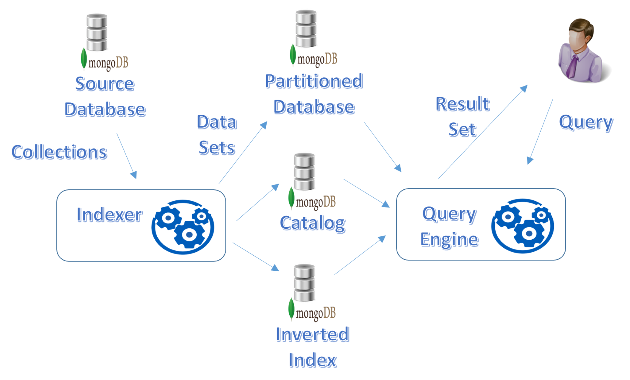
• Task 1: Database Scanning. First of all, as illustrated in Figure 3, the Source Database is scanned, in order to find out all the collections stored in it.
• Task 2: Schema Extraction and Identification of JSON Data Sets. Each collection in the Source Database is fully read; for each document, its schema is extracted, in order to identify the JSON data set which the document belongs to.
  The output of this task is the Partitioned Database (see Figure 3): the original collections in the Source Database are partitioned; in the Partitioned Database, we have one collection for each single JSON data set identified in the Source Database. This design choice is motivated by the need for efficiently evaluating JSON queries on JSON data sets (to select documents).
• Task 3: Catalog Construction. The JSON data sets identified in the previous task and their schemas are described in the Catalog (see Figure 3), so that the Query Engine can exploit it to drive the query process.
• Task 4: Indexing. The catalog is used to generate the Inverted Index (see Figure 3). Specifically, keys in the inverted index are names of collections and names of leaf fields (we do not consider field paths, because they cannot be expressed in the blind query q).

In Figure 3, for the sake of clarity we depicted four different databases. Of course, they could be fused in one single database. The HammerJDB framework is implemented on top of MongoDB; specifically, we adopted an intermediate solution, as far as the number of databases is concerned, that is, Partitioned Database, Catalog and Inverted Index are stored in the same MongoDB database, while the Source Database is not altered, to maintain separation between source data and service data.

Tasks 1, 2 and 3 are performed by the Partition_Collection procedure described in Algorithm 1. The procedure scans a given collection, identifies the JSON data sets within it and partitions the collection, that is, it generates as many collections in the Partitioned Database as the identified JSON data sets (one collection for each JSON data set) and copies the documents from the source collection to the proper (collection representing the corresponding) JSON data set. In the following, we describe the procedure in details.

• The procedure receives, as input parameter, a string denoting the name of the collection to scan.
• At lines 1 and 2, the $JDS$ variable is defined and initialized to the empty set; its role is to collect the full set of JSON data sets identified by the procedure.
• The For Each loop at lines 3 to 20 reads each single document d from the collection. On this document, many tasks are performed.

  -

  At line 4, the ExtractSchema function is called, to get a set of descriptors constituting the schema of the document. This function is reported in Algorithm 2.

  -

  The nested For Each loop at lines 6 to 11 checks for a JSON data set already present in set $JDS$ having the same schema as document d. If there exists such a JSON data set (line 6), the $found$ variable is set to true (line 8) and the $target\_jds$ variable is assigned with the descriptor of this JSON data set (line 9).

  -

  If there not exists a previous JSON data set in $JDS$ having the same schema as document d (line 12), a new JSON data set must be created. In details: a new identifier is generated (line 13), that is used to generate the name of the database collection (to create in the Partitioned Database) to store documents belonging to this JSON data set (line 14); the new collection is created (line 15) and the descriptor of this new JSON data set is assigned to the $target\_jds$ variable (line 16) to be added to the $JDS$ set (line 17).

  -

  Document d is copied into the collection storing the documents of the JSON data set which d belongs to (line 19).

• The last task performed by the Partition_Collection procedure is to add the descriptors of the JSON data sets so far generated into the Catalog database (line 21).

Algorithm 1: Procedure Partition_Collection.
	Procedure Partition_Collection($CollectionName$: String)
	Begin
1.	$JDS$: Set-of( data_set_descriptor )
2.	$JDS:=\varnothing$
3.	For Each$d\in$Collection( $CollectionName$ ) Do
4.	$ds:=$ ExtractSchema(d, ||)
5.	$found:=false$; $target\_jds:=null$
6.	For Each$jds\in JDS$Do
7.	If$|jds.schema\cap ds|=\left|ds\right|$ AND $|jds.schema|=\left|ds\right|$ Then
8.	$found:=true$
9.	$target\_jds:=jds$
10.	End If
11.	End For Each
12.	If$found=false$Then
13.	$new\_id:=$GenId()
14.	$new\_name:=CollectionName•new\_id$
15.	CreateCollection($CollectionName$)
16.	$target\_jds:=\langle new\_id,CollectionName,new\_name,ds\rangle$
17.	$JDS:=JDS\cup \{target\_jds\}$
18.	End If
19.	SaveToCollection(d, $target\_jds.name$)
20.	End For Each
21.	AddToCatalog($JDS$)
	End Procedure

Algorithm 2: Function ExtractSchema.
	Function ExtractSchema(d: document, $base$: path): Set-of( FieldDescriptor)
	Begin
1.	S: Set-of( FieldDescriptor)
2.	$S:=\varnothing$
3.	For Each$f\in$ Fields-of(d) Do
4.	$path:=base•f.name$
5.	If$f.type=$“document”Then
6.	$S:=S\cup$ExtractSchema( Vale-of( d, $f.name$), $path$)
7.	Else
8.	$descr:=\langle path,f.name,f.type\rangle$
9.	$S:=S\cup \left\{descr\right\}$
10.	End If
11.	End For Each
12.	ReturnS
	End Function

At line 4, the Partition_Collection procedure calls the Extract_Schema function, that is reported in Algorithm 2. It is a recursive function that receives two parameters: d is the document which to extract the schema from, while $base$ is the base path to extend with names of the fields in d. Line 4 of Algorithm 1 provides the empty path || as base path. The function returns a set of field descriptors, that represents the schema of the document.

We now describe the function in details.

• At lines 1 and 2, the S variable is defined and initialized to the empty set; its role is to collect fields descriptors.
• The For Each loop at lines 3 to 11 scans each (root) field f in document d. For each field, it performs several actions.

  -

  At line 4, the path of the field is generated, by appending the field name $f.name$ to the base path (by means of operator •).

  -

  If the (data) type of the field is “document” (line 5), this means that the value of the field is a nested document: the Extract_Schema function is recursively called (at line 6), by providing the value of the field and the new base path.

  -

  If the type of the field is not “document” (line 7), this means that its descriptor can be inserted into S: line 8 generates the descriptor, that is inserted into S at line 9.

• The function terminates by returning the set S of generated descriptors (line 12).

5.3. Query Engine

In order to find useful documents in the database, the user submits a blind query q (as in Definition 6) to the Query Engine, as illustrated in Figure 3. Based on Problem 2, it has to transform q into a pool of JSON queries (see Definition 12), that is, queries that refer to a JSON data set identifier and use field paths to refer to fields.

The main steps of the query rewriting process performed by the Query Engine are hereafter described.

• Step 1: Generation of Neighbour Queries. First of all, the blind query q is rewritten on the basis of the meta-data contained in the catalog, in order to obtain the set of queries to process Q, i.e., q and neighbour queries, as in Step 1 of the classical blind query process described in Section 4.2.2.
  In this step, we only exploit lexical and/or semantic similarities of terms in the catalog, in particular of field names, independently of their path (and, consequently, independently of the current, possibly complex, structure of documents).
  In a few words, we rewrite the original blind query q into a pool of partially-blind queries Q, that are likely to find some documents. These queries are partially blind, in the sense that they are obtained by considering terms actually present in the catalog, but still do not consider JSON data sets and their actual (possibly complex) structure.
• Step 2: VSM. Formalized by means of the Vector Space Model approach, each query $qp\in Q$ is used to search the Inverted Index. For each query $qp$, we obtain the set $JDS\left(qp\right)=\{jd{s}_1,jd{s}_2,\dots \}$ of JSON data sets that possibly match $qp$. Only the JSON data sets $jd{s}_i\in JC$ having a term relevance measure $krm(jd{s}_i,qp)\ge th\_krm$ ($th\_krm$ is the minimum threshold introduced in Section 4.2.2 for term relevance) are considered.
  The idea is that partially-blind queries obtained by rewriting the original blind query q are exploited to find out those JSON data sets that possibly can contain relevant documents.
• Step 3: Schema Fitting and Generation of JSON Queries. For each query $q{p}_i\in Q$ and each JSON data set $jd{s}_j\in JD\left(q{p}_i\right)$, the schema fitting degree $sfd(jd{s}_j,q{p}_i)$ is computed and the overall relevance measure $rm(jd{s}_j,q{p}_i)=\alpha \times krm(jd{s}_j,q{p}_i)+(1-\alpha )\times sfd(jd{s}_j,q{p}_i)$ is computed. If a JSON data set is such that $rm(jd{s}_j,q{p}_i)\ge th\_rm$ (where $th\_rm$ is the minimum threshold for the overall relevance measure, see Section 4.2.2), the new JSON query $j{q}_{i,j}$ is generated by assigning $j{q}_{i,j}.jds\_id=jd{s}_j.id$, as well as $j{q}_{i,j}.P$ and $j{q}_{i,j}.sc$ are obtained, respectively, from $q{p}_i.P$ and $q{p}_i.sc$ by replacing all field names with the corresponding field path (in case of a field name corresponding to multiple fields, the comparison predicate is replaced by a disjunction of predicates, one for each alternative field path). The final set $JQ=\bigcup \left\{j{q}_{i,j}\right\}$ of JSON queries is obtained.
  In this step, we perform a second rewriting process—partially-blind queries in Q are rewritten into a set of exact queries, that perfectly match the JSON data sets to query. This way, the next step can actually retrieve the JSON documents.
• Step4: Execution of JSON Queries. Each JSON query $j{q}_k\in JQ$ is executed. The result set $RS\left(j{q}_k\right)=\{d_1,d_2,\dots \}$ of JSON documents that satisfy the query is obtained. The final result set $RS={\bigcup }_{k}RS\left(j{q}_k\right)$ is generated, as the result set of the original blind query q (as asked by Problem 2).

The main novelty introduced in this paper, compared to our previous paper for blind querying of corpora of Open Data [3], is the second rewriting step, by means of which the queries in Q (that are still partially blind) are adapted to the actual structure of JSON data sets. This second rewriting step actually enables us to apply the technique for blind querying to NoSQL databases of JSON documents.

Listing 6. Complete example.

Blind Query

$q:\langle dn=$[Ads],

$P=\{$[ID], [Profession], [City]},

$sc=($[City]=“Valencia” AND [Country]=“Spain”$)\rangle$

Queries to Process

$q{p}_1:\langle dn=$[Ads],

$P=\{$[ID], [Profession], [City]},

$sc=($[City]=“Valencia” AND [Country]=“Spain”$)\rangle$

$q{p}_2:\langle dn=$[Ads],

$P=\{$[ID], [Job Title], [City]},

$sc=($[City]=“Valencia” AND [Country]=”Spain“$)\rangle$

$q{p}_3:\langle dn=$[Ads],

$P=\{$[ID], [Profession], [Location]},

$sc=($[Location]=”Valencia” AND [Country]=“Spain”$)\rangle$

Selected JSON Data Sets

$JD(q{p}_2=\varnothing$, $JD(q{p}_2=\{3,4\}$, $JD(q{p}_3=\left\{2\right\}$

JSON Queries

$j{q}_1:\langle jds\_id=$3,

$P=\{$|.“ID”|, |.“Job Title”|, |.“Area”.“City”|},

$sc=($|.“Area”.“City”|=“Valencia” AND |.“Area”.“Country”|=“Spain”$)\rangle$

$j{q}_2:\langle jds\_id=$4,

$P=\{$|.“ID”|, |.“Offer”.“Job Title”|, |.“Offer”.“Place”.“City”|},

$sc=($|.“Offer”.“Place”.“City”|=“Valencia” AND

|.“Offer”.“Place”.“Country”|=“Spain“$)\rangle$

$j{q}_3:\langle jds\_id=$2,

$P=\{$|.“ID”|, |.“Profession”|, |.“Place”.“Location”|},

$sc=($|.“Place”.“Location”|=“Valencia” AND |.“Place”.“Country”|=“Spain”$)\rangle$

Listing 6. Complete example.

Blind Query

$q:\langle dn=$[Ads],

$P=\{$[ID], [Profession], [City]},

$sc=($[City]=“Valencia” AND [Country]=“Spain”$)\rangle$

Queries to Process

$q{p}_1:\langle dn=$[Ads],

$P=\{$[ID], [Profession], [City]},

$sc=($[City]=“Valencia” AND [Country]=“Spain”$)\rangle$

$q{p}_2:\langle dn=$[Ads],

$P=\{$[ID], [Job Title], [City]},

$sc=($[City]=“Valencia” AND [Country]=”Spain“$)\rangle$

$q{p}_3:\langle dn=$[Ads],

$P=\{$[ID], [Profession], [Location]},

$sc=($[Location]=”Valencia” AND [Country]=“Spain”$)\rangle$

Selected JSON Data Sets

$JD(q{p}_2=\varnothing$, $JD(q{p}_2=\{3,4\}$, $JD(q{p}_3=\left\{2\right\}$

JSON Queries

$j{q}_1:\langle jds\_id=$3,

$P=\{$|.“ID”|, |.“Job Title”|, |.“Area”.“City”|},

$sc=($|.“Area”.“City”|=“Valencia” AND |.“Area”.“Country”|=“Spain”$)\rangle$

$j{q}_2:\langle jds\_id=$4,

$P=\{$|.“ID”|, |.“Offer”.“Job Title”|, |.“Offer”.“Place”.“City”|},

$sc=($|.“Offer”.“Place”.“City”|=“Valencia” AND

|.“Offer”.“Place”.“Country”|=“Spain“$)\rangle$

$j{q}_3:\langle jds\_id=$2,

$P=\{$|.“ID”|, |.“Profession”|, |.“Place”.“Location”|},

$sc=($|.“Place”.“Location”|=“Valencia” AND |.“Place”.“Country”|=“Spain”$)\rangle$

Example 7.

To illustrate the overall query process, consider Listing 6. Suppose the user wishes to find job ads related to the city of Valencia (Spain); he/she submits a blind query (denoted as q) in which the selection condition should select the documents having value “Valencia” for the [City] field and value “Spain” for the [Country] field; the properties (fields) of interest are [ID], [Profession] and [City].

Based on semantic similarity, the set of Queries to Process Q is generated. It contains three queries: $q{p}_1$ coincides with the blind query q; $q{p}_2$ is derived from q by replacing the [Profession] field with [Job Title]; query $q{p}_3$ is derived from q by replacing the [City] field with [Location].

Each query is evaluated by means of the Vector Space Model to retrieve possibly relevant JSON data sets; we refer to our sample database containing collections SouthernCountriesAds (Listing 2) and NorthernCountriesAds (Listing 3), as well as we refer to the JSON data sets reported in Listing 4 and Listing 5. Notice that query $q{p}_1$ does not retrieve any data set; query $q{p}_2$ retrieves the data sets 3 and 4 (Listing 5), while query $q{p}_3$ retrieves the data set 2 (Listing 4).

Consequently, three JSON queries are derived, as reported in Listing 6 and evaluated on the JSON data sets. Only query $j{q}_3$ retrieves some documents, that is, the two documents appearing in the JSON data set 2 (reported at the bottom of Listing 4).

6. Benchmark and Experiments

In this section, we first detail the real-life application context related to the analysis of data gathered from online job portals, that has inspired the examples reported in the paper; from these data sets, we built the data set used to test our approach. Then, we show and describe the results obtained from our experiments.

6.1. Application Context and Datas St

Online job portals are Web sites that collect and publish job offers (called Online Job Vacancies or OJVs). There are several categories of portals:

• Online job portals of Public Employment Services;
• Private online job portals operated either by national actors or by international consortia (e.g., Axel Springer Media);
• Aggregators gathering advertisements from other job portals and re-posting them on their own Web site (e.g., Jobrapido, Adzuna);
• Employment and recruiting agencies (e.g., Adecco, Randstad and Manpower);
• Newspapers maintaining their own online portals for job advertisements (e.g., Guardian Jobs);
• Online portals for classified ads, that is, small advertisements in categories such as “for sale”, “services”, “jobs” (e.g. Ebay and Subito).

In academic research, online job portals may provide researchers with precious information to study the labour market in real time [1].

However, gathering and analyzing information from the Web is difficult for various reasons. First of all, different sources provide data with different formats. Second, inconsistencies concerning OJVs easily occur, such as duplication of the same OJV on different portals, with different duration and so on. Consequently, representing OJVs as JSON documents and collecting them in a NoSQL database for JSON documents provides the necessary flexibility to manage them in an effective way.

Tabulaex [35], a labour market analytics company, collects data concerning job offers from thousands of Web-pages and many APIs. Its NoSQL database contains about 170 million job offers, gathered and cleaned from several European Web sites. Tabulex estimated the effort to gather and harmonize the structure of JSON documents into a unique and common structure by continuously following the changes that may appear in the monitored portals and APIs: only to maintain data gathering and harmonization from 13 sources, 6 man days per month of highly skilled people are necessary. These considerations inspired our work: harmonization of data could be avoided, if a tool for blind querying heterogeneous JSON documents were available.

In order to build the data set used for our tests, three subsets of raw data referring to different sources have been used for our experiments: the first is from a German Employment agency, the second from a Spanish Public Employment Service and the third refers to data gathered by an international job search engine. Only documents in English language have been considered.

• The German data set is composed by 1000 documents sampled from the data scraped from an Employment agency. This job offers are stored within the test database in a collection named “Jobs”.
• The second data set contains ads from the Spanish Public Employment Service. It contains 1000 documents. It is stored within the test database in the collection named “Spanish-jobs”.
• The data set from the international job search engine contains only job ads related to the Italian labour market. In the test database, the sample 1000 documents are stored in the collection named “Job-offers”.

In practice, the test database is managed by MongoDB; within it, we have three collections, named “Jobs”, “Spanish-jobs” and “Job-offers”, each one collecting 1000 JSON documents, for a total of 3000 documents describing JOVs with various formats. In this respect, to test the capability of our technique to seamlessly deal with different document structures, we inserted documents with four different structures into each single collection (specifically, four groups of 250 documents), by randomly partitioning each set of 1000 selected documents, so that documents in each group of 250 documents are restructured in the same way, by introducing nested structures as well.

6.2. Experiments

In order to evaluate the effectiveness of the approach, we performed several experiments on the test database previously described.

The experiments involved eight different queries, designed (see Listing 7) to stress the capability of the approach as detailed in the following:

Listing 7. Queries for the Experimental Evaluation.

$q_1:\langle dn=$[jobs],

$P=\{$[title], [place]},

$sc=($[lang] = “it” AND [publishdate] >= “2018-01-01”$)\rangle$

$q_2:\langle dn=$[jobs],

$P=\{$[title], [place], [country]},

$sc=($[description] = “Java” OR [title] = “Java”$)\rangle$

$q_3:\langle dn=$[vacancies],

$P=\{$[title], [description],[place], [country]},

$sc=($[place] = “Madrid” OR[place] = “Bilbao”$)\rangle$

$q_4:\langle dn=$[jobs],

$P=${$\left[\mathtt{title}\right],\left[\mathtt{description}\right],\left[\mathtt{place}\right],\left[\mathtt{country}\right]$} ,

$sc=($[contract] = “Permanent” AND[place] = “Milan”$)\rangle$

$q_5:\langle dn=$[jobs],

$P=\{$[title], [description],[place], [country]},

$sc=($[title] = “SAP Finance Expert” AND[country] = “DE”$)\rangle$

$q_6:\langle dn=$[joboffers],

$P=\{$[title], [description],[skills], [country]},

$sc=($[description] = “Oracle” OR[skills] = “Oracle”$)\rangle$

$q_7:\langle dn=$[jobS],

$P=\{$[title], [description],[contract], [place], [company]},

$sc=($[title] = “Fertigungsplaner” OR[title] = “Production Planner” OR

[title] = “Pianificatore della produzione” OR

[title] = “Planificador de Producción”$)\rangle$

$q_8:\langle dn=$[job-offer],

$P=\{$[title], [description],[industry], [place], [company]},

$sc=($[place] = “Berlin” OR[industry] = “IT”$)\rangle$

Listing 7. Queries for the Experimental Evaluation.

$q_1:\langle dn=$[jobs],

$P=\{$[title], [place]},

$sc=($[lang] = “it” AND [publishdate] >= “2018-01-01”$)\rangle$

$q_2:\langle dn=$[jobs],

$P=\{$[title], [place], [country]},

$sc=($[description] = “Java” OR [title] = “Java”$)\rangle$

$q_3:\langle dn=$[vacancies],

$P=\{$[title], [description],[place], [country]},

$sc=($[place] = “Madrid” OR[place] = “Bilbao”$)\rangle$

$q_4:\langle dn=$[jobs],

$P=${$\left[\mathtt{title}\right],\left[\mathtt{description}\right],\left[\mathtt{place}\right],\left[\mathtt{country}\right]$} ,

$sc=($[contract] = “Permanent” AND[place] = “Milan”$)\rangle$

$q_5:\langle dn=$[jobs],

$P=\{$[title], [description],[place], [country]},

$sc=($[title] = “SAP Finance Expert” AND[country] = “DE”$)\rangle$

$q_6:\langle dn=$[joboffers],

$P=\{$[title], [description],[skills], [country]},

$sc=($[description] = “Oracle” OR[skills] = “Oracle”$)\rangle$

$q_7:\langle dn=$[jobS],

$P=\{$[title], [description],[contract], [place], [company]},

$sc=($[title] = “Fertigungsplaner” OR[title] = “Production Planner” OR

[title] = “Pianificatore della produzione” OR

[title] = “Planificador de Producción”$)\rangle$

$q_8:\langle dn=$[job-offer],

$P=\{$[title], [description],[industry], [place], [company]},

$sc=($[place] = “Berlin” OR[industry] = “IT”$)\rangle$

• Query $q_1$ looks for job offers that are written in Italian, posted in the year 2018. We are interested in the properties named [title] and [place] (i.e., job location). Notice that the date is written as “2018-01-01”, to check and stress the search of similar terms.
• Query $q_2$ looks for job offers concerning Java developers. In particular, we are interested in job titles containing the term Java, as well as the job location. In fact, our goal (as analysts) may be to build a map with the distribution of vacancies and check the mismatching problem between supply and demand of Java developers. Notice the field named [description], that is not present in any data set stored in the database; we chose it because we wanted to specify a very generic field name.
• In query $q_3$ we look for job vacancies in Madrid and Bilbao.
• Query $q_4$ looks for data about Permanent position in Milan, in order to evaluate the type of contracts in the Italian labour market.
• In query $q_5$, we look for job offers in Germany, concerning experts in SAP Finance.
• Query $q_6$ is designed to obtain all job vacancies that contain the skill Oracle (related to Oracle Database or other Oracle products). Notice that, also in this case we use the [description] field name in the selection conditions, to stress our framework.
• To check the capability of our approach to scale over the corpus of the data, query $q_7$ looks for data about “Production Planner” in different languages on the same field ([title]).
• Finally, we wanted to specify another very generic field name, that is, [company]. In query $q_8$, we look for jobs posting in the IT industry sector in “Berlin”, in order to evaluate job offers in the ICT sector in the city of Berlin.

To perform the evaluation, we manually created a golden benchmark by analyzing and labeling every JSON object as relevant or not relevant with respect to each query (Tabulaex performs Machine Learning and AI models to categorize each job vacancy. Every result was evaluated in refers also to the labeled data provided by Tabulaex (see Reference [36])).

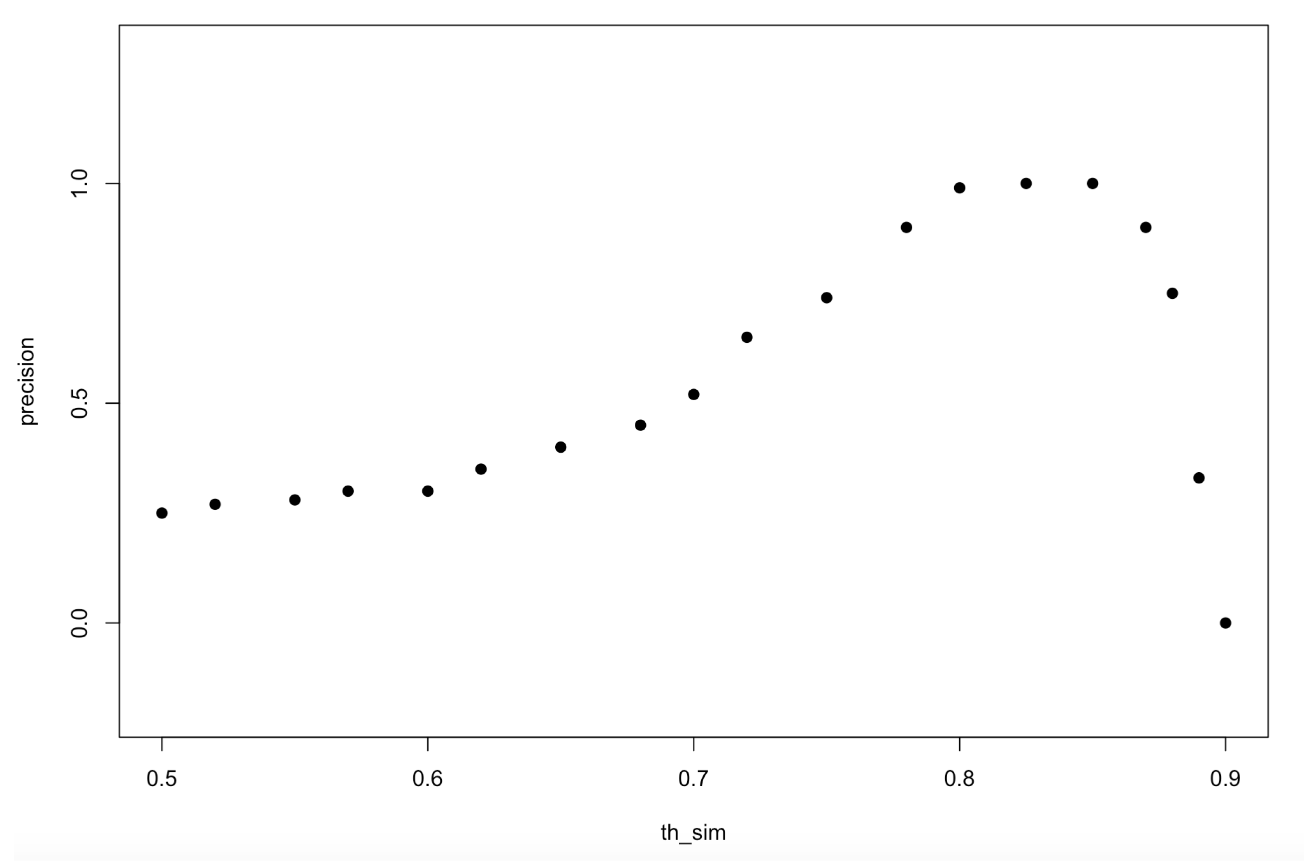
6.2.1. Sensitivity Analysis

We performed four tests to evaluate the effects of varying the thresholds introduced in Section 4.2. Hereafter, we recall the parameters and report the values we set.

• th_sim: it is the minimum threshold for the lexical similarity, we chose two distinct values, i.e., 0.8 and 0.9.
• th_krm: it is the minimum threshold for the Term-based Relevance Measure; we considered two different values, that is, 0.2 and 0.3.
• th_rm: it is the minimum threshold for the global relevance of data sets; we considered two different values, that is, 0.2 and 0.3.

We defined 4 configurations: these parameters derive from our previous researches about blind queries on Open Data Portals. We observed and reported the configurations that gave the best performance in terms of recall and precision scores. It is worth noticing that our main goal is to maximize the recall during the selection of JSON data sets and maximize the precision during the filtering of documents.

• For Test${}_1$, th_sim$=0.9$, th_krm$=0.3$ and th_rm$=0.3$;
• For Test${}_2$, th_sim$=0.9$, th_krm$=0.2$ and th_rm$=0.2$;
• For Test${}_3$, th_sim$=0.8$, th_krm$=0.3$ and th_rm$=0.3$;
• For Test${}_4$, th_sim$=0.8$, th_krm$=0.2$ and th_rm$=0.2$;

Note that the thresholds we used for defining the configurations are independent of the specific application domain. In fact, we used exactly the thresholds that in our previous works on Hammer [3,25] where considered to study the effectiveness of blind querying open data portals.

In

Table 1. Sensitivity Analysis for JSON Data Sets.

	Precision (%) for JSON Data Sets
Query	Test${}_{\mathbf{1}}$	Test${}_{\mathbf{2}}$	Test${}_{\mathbf{3}}$	Test${}_{\mathbf{4}}$
$q_1$	100.00	33.33	100.00	33.33
$q_2$	100.00	100.00	100.00	100.00
$q_3$	100.00	33.33	33.33	33.33
$q_4$	33.33	33.33	33.33	33.33
$q_5$	33.33	33.33	33.33	33.33
$q_6$	100.00	100.00	100.00	100.00
$q_7$	100.00	100.00	100.00	100.00
$q_8$	33.33	33.33	33.33	33.33

, we report the precision as far as the retrieval of JSON data sets is concerned, before the JSON documents are selected by evaluating the selection conditions. We do not report recall, because we obtained always a value of $100\%$: this means that the desired JSON data sets are always retrieved; therefore, precision becomes the key metric to be studied. In particular, we notice that in the case of queries $q_1$, $q_3$ and $q_4$, the reduction of the values for th_krm and th_rm (Test${}_2$ ad Test${}_4$), affects the performance, meaning that the model retrieves all the data sets and many more. Both recall and precision are insensitive to the variation of the th_sim parameter. We expected this behaviour, because neighbour queries are obtained by means of semantic similarity in this data set (while th_sim is the minimum threshold for lexical similarity).

Let us consider now the retrieval of single JSON documents (job offers).

Table 2. Sensitivity Analysis for Documents.

	Recall (%) for Documents
Query	Test${}_{\mathbf{1}}$	Test${}_{\mathbf{2}}$	Test${}_{\mathbf{3}}$	Test${}_{\mathbf{4}}$
$q_1$	100.00	100.00	100.00	100.00
$q_2$	100.00	100.00	100.00	100.00
$q_3$	n.c.	n.c.	100.00	100.00
$q_4$	n.c.	n.c.	100.00	100.00
$q_5$	100.00	100.00	100.00	100.00
$q_6$	n.c.	100.00	100.00	100.00
$q_7$	n.c.	100.00	50.00	50.00
$q_8$	100.00	100.00	100.00	100.00
	Precision (%) for Documents
Query	Test${}_{\mathbf{1}}$	Test${}_{\mathbf{2}}$	Test${}_{\mathbf{3}}$	Test${}_{\mathbf{4}}$
$q_1$	100.00	100.00	100.00	100.00
$q_2$	100.00	100.00	100.00	100.00
$q_3$	n.c.	n.c.	100.00	100.00
$q_4$	n.c.	n.c.	70.37	70.37
$q_5$	100.00	100.00	100.00	100.00
$q_6$	n.c.	27.78	27.78	27.78
$q_7$	n.c.	100.00	100.00	100.00
$q_8$	4.44	4.44	4.55	4.55

reports both recall and precision.

Note that most of the queries retrieve exactly the desired documents and nothing more. This is not true for query $q_4$. In particular, query $q_4$ retrieves some documents that are not related to the original query: this is because the query is formulated with the [contract] field; however, many documents do not have such a field, while contract information are (improperly) hidden within fields named [Working Hours]. In this case, it is difficult to disambiguate the two fields with a small collection of documents, as in our case.

Looking at the precision for query $q_3$, we notice that for Test${}_3$ and Test${}_4$ the thresholds th_sim set to 0.8 determines a precision of 100%, while increasing it to 0.9 causes the reduction of the search space, obtaining no documents in the result set (n.c. mean that zero documents are retrieved). Apparently, this could mean that increasing the minimum threshold for lexical similarity, the JSON data set containing the desired document is no longer retrieved. However, precision for JSON data sets is always 100%; thus, the JSON data containing the desired documents set is retrieved, but the blind query is not rewritten into the neighbour query that selects the proper field; consequently, the proper JSON query is not obtained and the desired documents are not retrieved.

From our experiments, we can conclude that our model behaves better with the Test${}_3$ configuration, that is, with th_sim = 0.8, th_krm = 0.3 and th_rm = 0.3. With th_krm = $0.2$, the VSM retrieval becomes too greedy and retrieves JSON data sets that are far away from the query.

The sensitivity to th_sim is limited by the fact that in Q (the set of queries to process) we keep only the 10 best neighbour queries with terms that are more similar to the alternative terms (synonyms): but a small increment of th_sim cause zero returned results; so it appears that it is better to set th_sim less or equal to $0.8$. To better understand how th_sim influences the behaviour, we investigated the relation between th_sim and precision with a grid search experiment based on Test${}_3$, that is, with th_krm = 0.3 and th_rm = 0.3, and th_sim is a sequence of numbers from 0.5 to 1.

Figure 4 shows the sensitivity of the precision with respect to the th_sim threshold. In particular, the precision increases when th_sim increases up to 0.85, after this point, precision dramatically decreases. This behaviour confirms what we said before; when th_sim becomes too high, the neighbour queries referring to field containing the desired values are no longer generated, so JSON queries that could select the desired documents are no longer generated too.

6.2.2. Comparison

The evaluation is compared with a suitable baseline. We identified two possible tools that could provide this baseline: Elasticsearch and Apache Solr.

Elasticsearch (https://www.elastic.co/) is a search engine based on Apache Lucene. It provides a distributed, multitenant-capable full-text search engine with an HTTP Web interface for schema-free JSON documents. It provides a scalable and near real-time search. Elasticsearch is completed by an analytics and visualization platform called Kibana. Default settings of Elasticsearch are very good; as an effect, it requires a very little configuration effort.

Apache Solr [37], is an open source enterprise search engine, developed on top of Apache Lucene. It is considered one of the best general purpose information retrieval tool currently available. However, it does not provide document selection, while JammerJDB does. Furthermore (the same holds for ElasticSearch) it is necessary to extract the data from the NoSQL database and upload them to Apache Solr, while HammerJDB directly works on the source JSON document store.

For our experiments, Elasticsearch was deployed on a virtual server with 4 virtual CPUs and 8 GB RAM. We had to change the Java Virtual Machine (JVM) options: specifically, we changed the heap size at 4 GB. Apache Solr was deployed on a similar virtual machine with 4 virtual CPUs and 8 GB RAM. Apache Solr required the installation of Java Runtime Environment (JRE) version 1.8. Both servers were hosted on a private cloud.

Table 3. Precision comparison of Test${}_3$ with the baselines obtained by means of Elasticsearch and Apache Solr (for JSON Data Sets).

Precision (%) for JSON Data Sets
Query	Elasticsearch	Apache Solr	Test${}_{\mathbf{3}}$
$q_1$	33.33	33.33	100.00
$q_2$	100.00	100.00	100.00
$q_3$	33.33	33.33	33.33
$q_4$	33.33	33.33	33.33
$q_5$	100.00	100.00	33.33
$q_6$	100.00	100.00	100.00
$q_7$	100.00	100.00	100.00
$q_8$	33.33	33.33	33.33

and

Table 4. Recall comparison of Test${}_3$ with the baselines obtained by means of Elasticsearch and Apache Solr (for Documents).

Recall (%) for Documents
Query	Elasticsearch	Apache Solr	Test${}_{\mathbf{3}}$
$q_1$	100.00	100.00	100.00
$q_2$	100.00	100.00	100.00
$q_3$	100.00	91.77	100.00
$q_4$	33.09	90.23	100.00
$q_5$	100.00	100.00	100.00
$q_6$	40.00	80.00	100.00
$q_7$	50.00	100.00	100.00
$q_8$	100.00	100.00	100.00
Precision (%) for Documents
Query	Elasticsearch	Apache Solr	Test${}_{\mathbf{3}}$
$q_1$	100.00	100.00	100.00
$q_2$	71.43	50.00	100.00
$q_3$	72.83	70.97	100.00
$q_4$	84.21	93.02	70.37
$q_5$	100.00	100.00	100.00
$q_6$	10.00	18.18	27.78
$q_7$	50.00	40.00	100.00
$q_8$	4.00	4.00	4.55

show the results of our comparison—Table 3 reports precision concerning the retrieval of JSON data sets (the recall is not reported, because we always obtained 100%); in Table 4, we reported recall (left side) and precision (right side) concerning document retrieval.

Concerning the precision and the recall measured on retrieved JSON data sets, we obtain the same performance with Elasticsearch and Apache Solr. HammerJDB performs better on query $q_1$; this means that the settings th_krm$=0.3$ and th_rm$=0.3$ allows the Query Engine of HammerJDB to better filter the data, by actually selecting the (wished) Italian job-offers and discarding the others.

Referring to recall and precision measured on the retrieved documents, the reader can see that our technique, when working with Test${}_3$ configuration, performs generally better, because Schema Fitting narrows the selected JSON data sets, better fitting the query condition with respect to documents structures.

So, we can conclude that HammerJDB can compete with Elasticsearch and Apache Solr, to effectively blind querying NoSQL databases of JSON documents. Not only, it does better, due to the capability of selecting specific documents of interest on the basis of selection conditions expressed in blind queries.

7. Discussion

Before concluding the paper, we want to discuss some critical issues concerning our approach.

• Stability of Sources. The application context described in Section 6.1 may suggest that data sources are stable in time; so, if we store documents coming from one single data source into a specific collection, they necessarily have the same structure.
  In practice, this is not true, in particular when the time window for gathering may span over years. In fact, if APIs are exploited to get documents, they could change the structure of the provided documents. Furthermore, if screen scraping techniques are used to get data from web sites that do not provide APIs, the situation may be even worse, because web interfaces change more frequently than APIs (sometimes they add more information, sometimes they reduce it); as an effect, JSON documents obtained by scraping the same site in different times may have different structures. Consequently, documents in the same collection may have different structures, due to the fact that the source is unstable.
• No control on choices. Why has a JSON document database been chosen? Why have other NoSQL databases like Entity Databases not been considered by the organization? For many reasons, that often are not technical. For example, one could be that analysts are already more familiar with the document database technology or, specifically, with MongoDB. A second reason could be that at the beginning of the gathering they had only JSON documents to deal with. A third reason could be that they inherited the choice from previous projects and so on.
  The cost of transforming (possibly partially unknown) heterogeneous databases into a homogeneous and simplified representation could be very high, both in terms of time (necessary to accurately inspect the data sets, and select, extract, restructure and load data) and in terms of money (the cost of people with the necessary skills, such as programmers, database experts, and so on, involved in the process).
• Neighbour Queries and Execution Times. Neighbour queries and related JSON queries must be executed and this, of course, significantly increases the execution times if compared to the execution of one single query.
  But in order to execute one single query, it would be necessary to have no heterogeneity in the data, that is, data should be pre-processed and collected into one single collection. However, as stated in the previous point, pre-processing could be very expensive. The goal of blind querying based on neighbour queries and JSON queries is to save pre-processing steps: in fact, even though the user had to wait for (let us say) 10 min, this would certainly be more convenient than spending working days in pre-processing. This is perfectly aligned with the spirit of information retrieval.
• HammerJDB versus ElasticSearch and Apache Solr. The reader could observe that the gain in accuracy obtained by HammerJDB with respect to ElasticSearch and Apache Solr could be not so relevant, so why not to use them? In fact, ElasticSearch and Apache Solr are famous to return results quite immediately.
  However, the reader should consider a different aspect of the problem; they have their own storage systems and data must be transferred from the JSON document store to them, thus causing the duplication of the data sets. Furthermore, performing this transfer is a trouble when the JSON store is continuously fed, because only incremental data must by transferred. Consequently, the version of the data sets in the JSON document store could be not aligned with the version queried by ElasticSearch or Apache Solr.
  The adoption of HammerJDB avoids this possibly expensive trasfer, because it directly works on the original JSON document database to query.
• Arrays are not supported. At the current stage of development of the blind query technique, array fields in JSON documents are not supported. Clearly, this is a sever limitation, in particular when documents describing GeoJSON [38] layers are stored. Transformations of JSON documents suggested in Section 5 totally or partially loose the original documents; in many applications, this loss could be a problem for further analysis activities. In this paper, we demonstrated that concepts defined in our previous work can be adapted to query JSON document databases, provided that array fields are not considered. In future work, we will deeply investigate how to effectively deal with array fields.

8. Conclusions and Future Work

This paper presents HammerJDB, a novel framework for blind querying NoSQL databases of JSON documents. The framework is a revamping of the Hammer framework [3] (originally introduced in Reference [2]), designed to introduce a technique for blind querying Open Data portals.

Specifically, the novel HammerJDB framework changes the application context, considering a NoSQL database for JSON documents as source to query, so as to extract JSON documents stored within it. It is based on the same basic technique for query rewriting, but it introduced a second step of query rewriting, in order to obtain queries (called JSON queries) that can be directly executed on JSON documents. In particular, JSON documents are pre-processed, in order to partition them into JSON data sets, that is, homogeneous sets of documents (on the basis of their schema).

To validate the approach, we performed some experiments on the data set collecting job offers, provided by Reference [35]. A pool of 8 queries allowed us to prove the efficacy of our approach. We compared our technique with two distinct baselines, that is, Elasticsearch and Apache Solr. We observed that our technique performs generally better, specifically as far as retrieval of documents is concerned.

As a future work, we plan to investigate how to deal with array fields; in fact, our technique is currently unable to deal with them.

As far as longer term activities are concerned, first of all we plan to improve our approach, in particular to better cope with a reduced number of collections or data sets. In order to improve both precision and recall, we are studying to apply Machine Learning models and Deep Learning to create a corpus of metadata, by reading the content of each dimension of each document (see References [39,40]). In our idea, we could use a pre-trained NLP model like BERT ([41]) to better understand user questions.

Second, we would like to exploit explicit correlations between terms, that can be obtained by performing a preliminary analysis of correlated terms in the meta-data catalog.

Third, we would like to fully exploit field paths, in order to consider names of intermediate fields and not only of leaf fields.

References

1. Boselli, R.; Cesarini, M.; Marrara, S.; Mercorio, F.; Mezzanzanica, M.; Pasi, G.; Viviani, M. WoLMIS: A labor market intelligence system for classifying web job vacancies. J. Intell. Inf. Syst. 2018, 51, 477–502. [Google Scholar] [CrossRef]
2. Pelucchi, M.; Psaila, G.; Toccu, M.P. Building a query engine for a corpus of open data. In Proceedings of the WEBIST 2017, 13th International Conference on Web Information Systems and Technologies, Porto, Portugal, 25–27 April 2017; pp. 126–136. [Google Scholar]
3. Pelucchi, M.; Psaila, G.; Toccu, M. Enhanced Querying of Open Data Portals. In Proceedings of the International Conference on Web Information Systems and Technologies, Porto, Portugal, 25–27 April 2017; pp. 179–201. [Google Scholar]
4. Zadeh, L.A. Fuzzy sets as a basis for a theory of possibility. Fuzzy Sets Syst. 1978, 1, 3–28. [Google Scholar] [CrossRef]
5. Damiani, E.; Tanca, L. Blind Queries to XML Data. In Proceedings of the 11th International Conference on Database and Expert Systems Applications, DEXA 2000, London, UK, 4–8 September 2000; pp. 345–356. [Google Scholar]
6. Damiani, E.; Lavarini, N.; Marrara, S.; Oliboni, B.; Pasini, D.; Tanca, L.; Viviani, G. The APPROXML Tool Demonstration. In Proceedings of the Advances in Database Technology—EDBT 2002, 8th International Conference on Extending Database Technology, Prague, Czech Republic, 25–27 March 2002; pp. 753–755. [Google Scholar]
7. Campi, A.; Damiani, E.; Guinea, S.; Marrara, S.; Pasi, G.; Spoletini, P. A fuzzy extension of the XPath query language. J. Intell. Inf. Syst. 2009, 33, 285–305. [Google Scholar] [CrossRef]
8. Marrara, S.; Pasi, G. Fuzzy Approaches to Flexible Querying in XML Retrieval. Int. J. Comput. Intell. Syst. 2016, 9, 95–103. [Google Scholar] [CrossRef] [Green Version]
9. Baumgartner, R.; Gatterbauer, W.; Gottlob, G. Web Data Extraction System. In Encyclopedia of Database Systems; Liu, L., Özsu, M.T., Eds.; Springer: Boston, MA, USA, 2009; pp. 3465–3471. [Google Scholar] [CrossRef]
10. Ferrara, E.; De Meo, P.; Fiumara, G.; Baumgartner, R. Web data extraction, applications and techniques: A survey. Knowl. Based Syst. 2014, 70, 301–323. [Google Scholar] [CrossRef] [Green Version]
11. Azad, H.K.; Deepak, A. Query expansion techniques for information retrieval: A survey. Inf. Process. Manag. 2019, 56, 1698–1735. [Google Scholar] [CrossRef] [Green Version]
12. Lee, H.M.; Lin, S.K.; Huang, C.W. Interactive query expansion based on fuzzy association thesaurus for web information retrieval. In Proceedings of the 10th IEEE International Conference on Fuzzy Systems, Melbourne, Australia, 2–5 December 2001; Volume 2, pp. 724–727. [Google Scholar]
13. Theobald, M.; Weikum, G.; Schenkel, R. Top-k query evaluation with probabilistic guarantees. In Proceedings of the Thirtieth International Conference on Very Large Data Bases-Volume 30, VLDB Endowment, Toronto, ON, Canada, 31 August–3 September 2004; pp. 648–659. [Google Scholar]
14. Cui, H.; Wen, J.R.; Nie, J.Y.; Ma, W.Y. Probabilistic query expansion using query logs. In Proceedings of the 11th International Conference on World Wide Web, Honolulu, HI, USA, 7–11 May 2002; ACM: New York, NY, USA, 2002; pp. 325–332. [Google Scholar]
15. Chum, O.; Mikulik, A.; Perdoch, M.; Matas, J. Total recall II: Query expansion revisited. In Proceedings of the 2011 IEEE Conference on Computer Vision and Pattern Recognition (CVPR), Colorado Springs, CO, USA, 20–25 June 2011; pp. 889–896. [Google Scholar]
16. Chum, O.; Philbin, J.; Sivic, J.; Isard, M.; Zisserman, A. Total recall: Automatic query expansion with a generative feature model for object retrieval. In Proceedings of the 2007 IEEE 11th International Conference on Computer Vision, Rio de Janeiro, Brazil, 14–21 October 2007; pp. 1–8. [Google Scholar]
17. Liu, J.; Dong, X.; Halevy, A.Y. Answering Structured Queries on Unstructured Data; WebDB 2006; Citeseer: Chicago, IL, USA, 2006; Volume 6, pp. 25–30. [Google Scholar]
18. Kononenko, O.; Baysal, O.; Holmes, R.; Godfrey, M. Mining Modern Repositories with Elasticsearch; MSR: Hyderabad, India, 2014. [Google Scholar]
19. Białecki, A.; Muir, R.; Ingersoll, G.; Imagination, L. Apache Lucene 4. In Proceedings of the SIGIR 2012 Workshop on Open Source Information Retrieval, Portland, OR, USA, 16 August 2012; p. 17. [Google Scholar]
20. Nagi, K. Bringing search engines to the cloud using open source components. In Proceedings of the 2015 7th International Joint Conference on Knowledge Discovery, Knowledge Engineering and Knowledge Management (IC3K), Lisbon, Portugal, 12–14 November 2015; Volume 1, pp. 116–126. [Google Scholar]
21. Pelucchi, M.; Psaila, G.; Maurizio, T. The challenge of using map-reduce to query open data. In Proceedings of the 6th International Conference on Data Science, Technology and Applications (DATA 2017), Madrid, Spain, 24–26 July 2017; pp. 331–342. [Google Scholar]
22. Dean, J.; Ghemawat, S. MapReduce: A flexible data processing tool. Commun. ACM 2010, 53, 72–77. [Google Scholar] [CrossRef]
23. Vavilapalli, V.K.; Murthy, A.C.; Douglas, C.; Agarwal, S.; Konar, M.; Evans, R.; Graves, T.; Lowe, J.; Shah, H.; Seth, S.; et al. Apache hadoop yarn: Yet another resource negotiator. In Proceedings of the 4th Annual Symposium on Cloud Computing, Santa Clara, CA, USA, 1–3 October 2013; ACM: New York, NY, USA; p. 5. [Google Scholar]
24. Zaharia, M.; Chowdhury, M.; Franklin, M.J.; Shenker, S.; Stoica, I. Spark: Cluster computing with working sets. HotCloud 2010, 10, 95. [Google Scholar]
25. Pelucchi, M.; Psaila, G.; Toccu, M. Hadoop vs. Spark: Impact on Performance of the Hammer Query Engine for Open Data Corpora. Algorithms 2018, 11, 209. [Google Scholar] [CrossRef]
26. Davoudian, A.; Chen, L.; Liu, M. A survey on NoSQL stores. ACM Comput. Surv. (CSUR) 2018, 51, 40. [Google Scholar] [CrossRef]
27. Bray, T. The Javascript Object Notation (Json) Data Interchange Format. 2014. Available online: https://buildbot.tools.ietf.org/html/rfc7158 (accessed on 15 March 2019).
28. Bordogna, G.; Capelli, S.; Psaila, G. A big geo data query framework to correlate open data with social network geotagged posts. In Proceedings of the The Annual International Conference on Geographic Information Science, Buffalo, NY, USA, 2–4 August 2017; Springer: Cham, Germany, 2017; pp. 185–203. [Google Scholar]
29. Bordogna, G.; Ciriello, D.E.; Psaila, G. A flexible framework to cross-analyze heterogeneous multi-source geo-referenced information: The J-CO-QL proposal and its implementation. In Proceedings of the International Conference on Web Intelligence, Leipzig, Germany, 23–26 August 2017; ACM: New York, NY, USA, 2017; pp. 499–508. [Google Scholar]
30. Bordogna, G.; Capelli, S.; Ciriello, D.E.; Psaila, G. A cross-analysis framework for multi-source volunteered, crowdsourced, and authoritative geographic information: The case study of volunteered personal traces analysis against transport network data. Geo-Spat. Inf. Sci. 2018, 21, 257–271. [Google Scholar] [CrossRef]
31. Psaila, G.; Fosci, P. Toward an Analist-Oriented Polystore Framework for Processing JSON Geo-Data. In Proceedings of the IADIS International Conference Applied Computing, Budapest, Hungaria, 21–23 October 2018; pp. 213–222. [Google Scholar]
32. Winkler, W.E. String Comparator Metrics and Enhanced Decision Rules in the Fellegi-Sunter Model of Record Linkage. In Proceedings of the Section on Survey Research Methods; American Statistical Association: Alexandria, VA, USA, 1990; pp. 354–359. [Google Scholar]
33. Miller, G.A. WordNet: A lexical database for English. Commun. ACM 1995, 38, 39–41. [Google Scholar] [CrossRef]
34. Manning, C.D.; Raghavan, P.; Schütze, H. Introduction to Information Retrieval; Cambridge University Press: Cambridge, UK, 2008; Volume 1. [Google Scholar]
35. Tabulaex; Tabulaex: Milano, Italy, 2018.
36. Amato, F.; Boselli, R.; Cesarini, M.; Mercorio, F.; Mezzanzanica, M.; Moscato, V.; Persia, F.; Picariello, A. Challenge: Processing web texts for classifying job offers. In Proceedings of the 2015 IEEE International Conference on Semantic Computing (ICSC), Anaheim, CA, USA, 7–9 February 2015; pp. 460–463. [Google Scholar]
37. Shahi, D. Apache Solr: An Introduction. In Apache Solr; Springer: Berlin, Germany, 2015; pp. 1–9. [Google Scholar]
38. Butler, H.; Daly, M.; Doyle, A.; Gillies, S.; Schaub, T.; Schmidt, C. Geojson Specification. Geojson.org. 2008. Available online: https://tools.ietf.org/html/rfc7946 (accessed on 15 March 2019).
39. Bojanowski, P.; Grave, E.; Joulin, A.; Mikolov, T. Enriching Word Vectors with Subword Information. Trans. Assoc. Comput. Linguist. 2017, 5, 135–146. [Google Scholar] [CrossRef] [Green Version]
40. Mikolov, T.; Chen, K.; Corrado, G.; Dean, J. Efficient estimation of word representations in vector space. arXiv 2013, arXiv:1301.3781. [Google Scholar]
41. Devlin, J.; Chang, M.W.; Lee, K.; Toutanova, K. Bert: Pre-training of deep bidirectional transformers for language understanding. arXiv 2018, arXiv:1810.04805. [Google Scholar]
Figure 1. Application Scenario of the HammerJDB framework.
Information 10 00291 g001
Figure 2. Original retrieval approach implemented within the former Hammer framework.
Information 10 00291 g002
Figure 3. Retrieval approach on top of JSON Document Stores implemented in the HamerJDB framework.
Information 10 00291 g003
Figure 4. Sensitivity of precision w.r.t. threshold th_sim.
Information 10 00291 g004