Key Performance Indicators for the Upgrade of Existing Coastal Defense Structures

Abstract

Due to the effects of climate change on the sea levels and on the frequency and intensity of extreme weather events, many coastal defense structures are expected to be exposed to increased loads with respect to their design conditions in the near future and need to be upgraded. Often, several design alternatives are available, and the identification of the ideal solution is not straightforward. Solutions that are effective in reducing overtopping and ensuring hydraulic safety may reduce or compromise the structural performance. Solutions that are both hydraulically and structurally effective may be extremely expensive and/or environmentally harmful. Using consolidated techniques of Multi-criteria analysis, this contribution proposes a simple methodology to consistently compare and rank the performance of several alternative approaches to upgrade existing structures, and to individuate the best solution. The proposed methodology consists of Key Performance Indicators (KPIs) of alternative solutions of upgrades, considering the reduction in the wave overtopping discharge (q) and the wave forces (F) by limiting costs and environmental impact. The definition of the KPIs was developed on the basis of new experimental data of q and F at dikes with crown walls and parapets, but it can be applied to various structure types, sea levels, and wave conditions. The application of the KPIs to the new experiments prompts a few conclusions of practical utility concerning the effectiveness of berms, crown walls, and parapets as elements to upgrade existing dikes.

1. Introduction

The control of wave overtopping is unquestionably one of the key aspects in the design of coastal defenses. Increasing evidence indicates that global climate change will alter sea winds and swell waves, modifying the violence and the frequency of storm events [1]. In most cases, the literature estimates of increases to coastal impacts are attributed to sea level rise [2,3] and rarely to changes to waves alone. Timmermans et al. [4] compared satellite observations to computer simulations and buoy measurements, finding important discrepancies in the reported average global wave conditions, raising questions about the uncertainty in these products. However, they [4] found coherent trends among the different prevision products in some regions—especially close to land and sea ice margins. In particular, strong positive trends of variation in the wave heights are expected in the Southern Ocean’s Atlantic Sector (southwest of Africa), in the Northwest Atlantic Ocean (east coast of North America), in the Western Pacific Ocean (southwest of Asia), and in the Mediterranean Sea. In these areas, the variations in the mean significant wave height (H_s) trends are estimated between 0.01 and 0.03 m/year, according to the geographical area and the prevision products. O’Grady et al. [5] recently analyzed incremental change signals in extreme wave heights to predict changes in the frequency of events, finding that the largest increases were typically experienced at higher latitudes. Similarly, Lobeto et al. [6] found that despite the underlying uncertainty characterizing extreme scenarios, significant changes in extreme H_s are expected over more than ~25% of the ocean surface, with an increasing H_s gradient from the equator to higher latitudes. According to [6], the maximum changes are expected in the northernmost regions of the Atlantic and Pacific oceans, with predictions of H_s reaching 19 and 22 m for the 20- and the 100-year return period scenarios, respectively. Similarly, the Southern Ocean presents values up to 17 and 20 m.

In such a context, many of the existing coastal defense structures are therefore likely to be exposed in the near future to increased loads due to the global sea level rise and, locally, to increasing incidence of extreme events. The effects on the structures will be various and hazardous, affecting the structural and the geotechnical stability and the hydraulic safety of the inland areas. For example, at rubble mound structures, higher loads may generate or exacerbate the damage state, inducing the partial or total collapse of the armor layer. For smooth defenses, higher loads may cause extra and/or more brittle and swift failure paths to the structures. Higher loads may also generate increased scour phenomena, at both the seaward and landward toe areas, if the structure is overtopped. Increased sea levels, combined with the storm surge and potentially extreme wave heights, can clearly compromise the structures hydraulic safety, triggering more or less catastrophic scenarios of coastal flooding.

To protect coastal areas from the several risks connected to climate change, the coastal defenses that were built decades ago to survive less severe storm conditions need to be updated and upgraded to ensure adequate protection from the risk of coastal flooding. Ideally, increasing the structures freeboard would represent the easiest and most effective solution to reduce wave overtopping. However, such a solution might be impracticable for social, economic, environmental, and feasibility reasons, and might not be effective to face the increased loads. Based on the site wave climate and the local specificities, various alternatives to freeboard extension have been investigated in the literature on the upgrading of existing structures: introduction of berms, front reservoirs, artificial reefs [7], overspill basins [8], retrofitting [9], etc. One possibility is represented by the inclusion of overhanging parts (recurve/parapet/wave return wall/bullnose) on top of seawalls (i.e., [10,11]), breakwaters [11,12,13], or dikes [14,15], resulting in an effective measure to reduce the wave overtopping discharge (q). However, the confined return flow induced by the presence of such overhanging parts may cause impulsive pressures and severe increases in the wave forces (F) at the walls [16,17,18]. The consequences for the overall structural stability may be extremely serious, especially in the event that the design load is reached and brittle failure paths are triggered. The reduction in overtopping is therefore sometimes incompatible with the limitation of the wave loads at the structures. This factor significantly complicates the choice of the most suitable solution to upgrade existing structures, even when the alternatives could be limited by local constraints. The matter is further complicated when considering that the “best” solution from an engineering point of view may be impracticable due to its environmental or aesthetic impact, and/or for its economic costs.

To support coastal engineers in the design phase of structural upgrades, a methodology to quickly and effectively individuate the optimal solution—simultaneously optimizing the reduction in overtopping, preserving the structural performance, and limiting costs and environmental impact—would be useful. To develop such a methodology, experiments specifically dedicated to the assessment of the integrated (i.e., structural and hydraulic) performance of coastal structures are needed. Unfortunately, the literature on this topic is poor, and the available data are extremely limited. To the author’s knowledge, the only studies including the simultaneous measurements of q and F are: (i) the experiments conducted by Pedersen et al. [8] on wave overtopping and wave forces on crown walls on top of differently armored mound breakwaters (rock, cube, and dolos); (ii) the small-scale 2D tests carried out by Smolka et al. [19] against a cube- and Cubipod^®-armored mound breakwater, measuring the data of the dimensionless horizontal and uplift forces and of the overturning moments at the crown wall; (iii) the regular and irregular tests of wave overtopping against a seawall with a variously inclined recurved parapet conducted by Martinelli et al. [17].

Nevertheless, none of these studies considered the combined measurements of q and F from an integrated point of view. Pedersen [12] conducted separate analyses of the effects of the crown walls on the overtopping and the wave loads, while Molines et al. [13], focusing principally on structural aspects, used the data of q alone to characterize the experiments in comparison to the literature. Based on the datasets by Pedersen [12] and Smolka et al. [19], Molines et al. [20] investigated for the first time the correlation between q and F at walls through the support of an artificial neural network; however, in this work, the q-values are still considered as “input data” of the artificial neural network to calculate the wave forces, and no integrated discussion is drawn.

Starting from this finding, Formentin and Zanuttigh [21] conducted a series of small-scale laboratory tests on smooth dikes upgraded with crown walls, sloping parapets, and berms, simultaneously measuring q and F at the crown walls. The setup of the configurations of these tests was specifically conceived to facilitate a systematic, parametric analysis of the effects of berms, crown walls, and parapets as potential upgrades to smooth dikes to improve their hydraulic and structural effectiveness in the face of increased wave loads and sea levels. Based on these experiments, this contribution proposes a new method to compare the integrated performance of several alternative forms of structural upgrades. This new method is based on the definition of quantitative Key Performance Indicators (KPIs) associated with each alternative solution of structural upgrade. These KPIs are calculated on the basis of the values of q and F, and of the estimations of the costs and the environmental impact related to each upgrade configuration with respect to the original one representing the existing structure to be upgraded. The method of calculating and assigning the KPIs follows the approach of Multi-Criteria Analysis and was conceived to be as general as possible. The main objective of this paper is to promote the use of the KPIs as a simple but effective method to support coastal engineers not only in the preliminary design phase of structural upgrades, but also in any applications in the maritime engineering field that may require the identification of an “optimal solution” from among alternatives. Examples of applications of a KPI-based methodology may range from the development of risk–cost-optimized maintenance strategies during the service life of coastal defenses [22], to the assessment of the damage in rubble mound scour protections [23], to the identification of the optimal layout for the inclusion of wave energy converters in breakwaters [24], etc.

This paper is organized as follows: Section 2 is dedicated to the description of the experiments and to the presentation of the data on q and F considered in this work in comparison to existing similar tests and predictive formulae. Section 3 proposes an integrated analysis and discussion of the combined effects on the overtopping and wave loads from introducing or upgrading structural elements such as berms, crown walls, and parapets. The definition of the KPIs is illustrated in Section 4. The overall methodology is applied to the data [21], and to other datasets from the literature, in Section 5. The conclusions of the work are drawn in Section 6.

2. The Database

The new method proposed in this contribution was mainly developed on the basis of a database of small-scale experiments on wave overtopping and wave loads at smooth, plain dikes upgraded with berms, crown walls, and parapets. The details of the experiments and the data of the wave overtopping discharge (q) and of the wave forces at the walls (F) have already been presented and discussed in previous articles (most recently, by Formentin et al. [25]). The characteristics of the tested configurations and of the structural upgrades—which are fundamental in order to follow the illustration of the new method (Section 4)—are briefly recalled in Section 2.1. while the experimental setup and the measurements performed are summarized in Section 2.2. The data of q and of F are presented in Section 2.3. in comparison with existing data and methods.

2.1. Tested Configurations

A total of 128 small scale experiments on wave overtopping and impact loads at walls were carried out in the wave flume of the Hydraulic Laboratory of the University of Bologna (Unibo). The experiments were conducted in accordance with the Froude similarity law, with reference to a hypothetical prototype structure of a smooth dike with a berm, crown wall, and parapet. The size and geometry of these structures may reproduce a typical prototype Dutch dike (see Jonkman et al. [26]) in 1:20 scale).

The structures tested in the lab were smooth dikes with a horizontal berm width (B) and a crown wall installed at the berm’s inshore edge, as illustrated in Figure 1. The structures were all built from Plexiglas (giving a roughness factor of γ_f = 1), and the walls were deeply clamped in the berm to avoid overturning.

The setup of the tested conditions was the result of a long-term project studying the overtopping discharge and the overtopping flow characteristics at dikes, which started with Formentin and Zanuttigh [21]. The geometry of the dikes was originally inspired by the experiments on dikes carried out at a 1:10 scale by Schüttrumpf and Oumeraci [27] in the small wave flume of the Technical University of Braunschweig. The inclusion of the crown walls was inspired by Van Doorslaer et al. [14], aiming at extending the study of the effects of crown walls and bullnoses on configurations other than the classical Belgian coastal defenses [15]. The original dimensions of the dikes [27] and of the walls [14] were rescaled to 1:20 to fit the size of the laboratory facility (see Section 2.2).

The ranges of the berm elevations (h_b) to the still water level and of the wave heights (H_s) were set up to investigate the effects of climate change in terms of sea level rise and increased wave heights, within the limits imposed by the constraints of the laboratory facility (H_s ≤ 0.06 m, corresponding to 1.2 m at prototype scale, and water depth in the channel h ≤ 0.40 m). According to the latest report from the United Nations’ Intergovernmental Panel on Climate Change (IPCC), the global mean sea levels will most likely rise by between 0.29 and 1.1 m by the end of the 21st century [1]. Starting from a standard, common condition of the berm’s relative emergence of h_b/H_s = −0.5, an intermediate scenario of a mean sea level rise of 0.60 m was considered. By rescaling this value to the model-scale value of 0.03 m, a configuration with the berm level corresponding to the still water level, h_b/H_s = 0, was designed. As for the wave heights, under the RCP4.5 (Representative Concentration Pathways) global warming scenario, the average magnitudes of the projected positive changes in the H_s-values may vary between + 0 m and + 0.3 m, and in most cases the changes are lower than 25% [6]. Following these previsions and starting from the moderate value of H_s = 0.05 m allowed by the lab facility, a second scenario of H_s = 0.06 m (+0.2 m at prototype scale and +25% of relative variation) was considered.

The structures height, from the bottom of the channel to the berm level (h_c in Figure 1), is the only geometrical parameter that was kept constant for all of the tests, and was equal to 0.35 m. All of the other parameters were varied, starting from four “basic” configurations of dikes without upgrades, as portrayed in Figure 2. All four of the basic configurations are characterized by a berm width B = 0.15 m and a crown wall height h_w = 0.04; their geometry varies for the dike slope-cot(α_d) = 2 or 4—and for the berm’s relative emergence-h_b/H_s = 0 or h_b/H_s = −0.5.

For brevity, the four “basic configurations” shown in Figure 2a–d will be referred to as c2h_b0, c2h_b05, c4h_b0, and c4h_b05, respectively. The configurations c2h_b0 and c4h_b0 represent climate change scenarios for rising sea levels. Starting from the four basic configurations, seven combinations of “structural upgrades” were investigated to address the effects of climate change in terms of increased wave heights and loads:

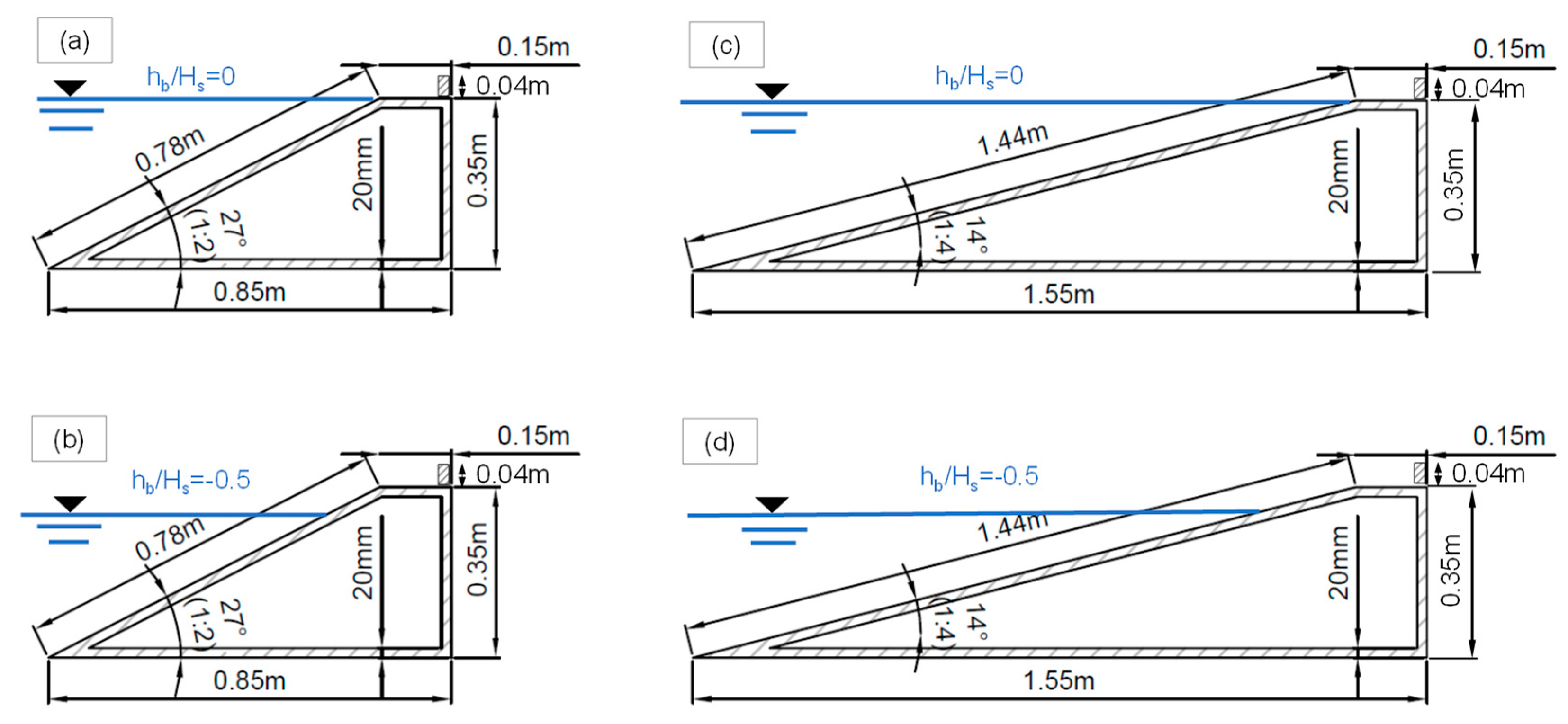
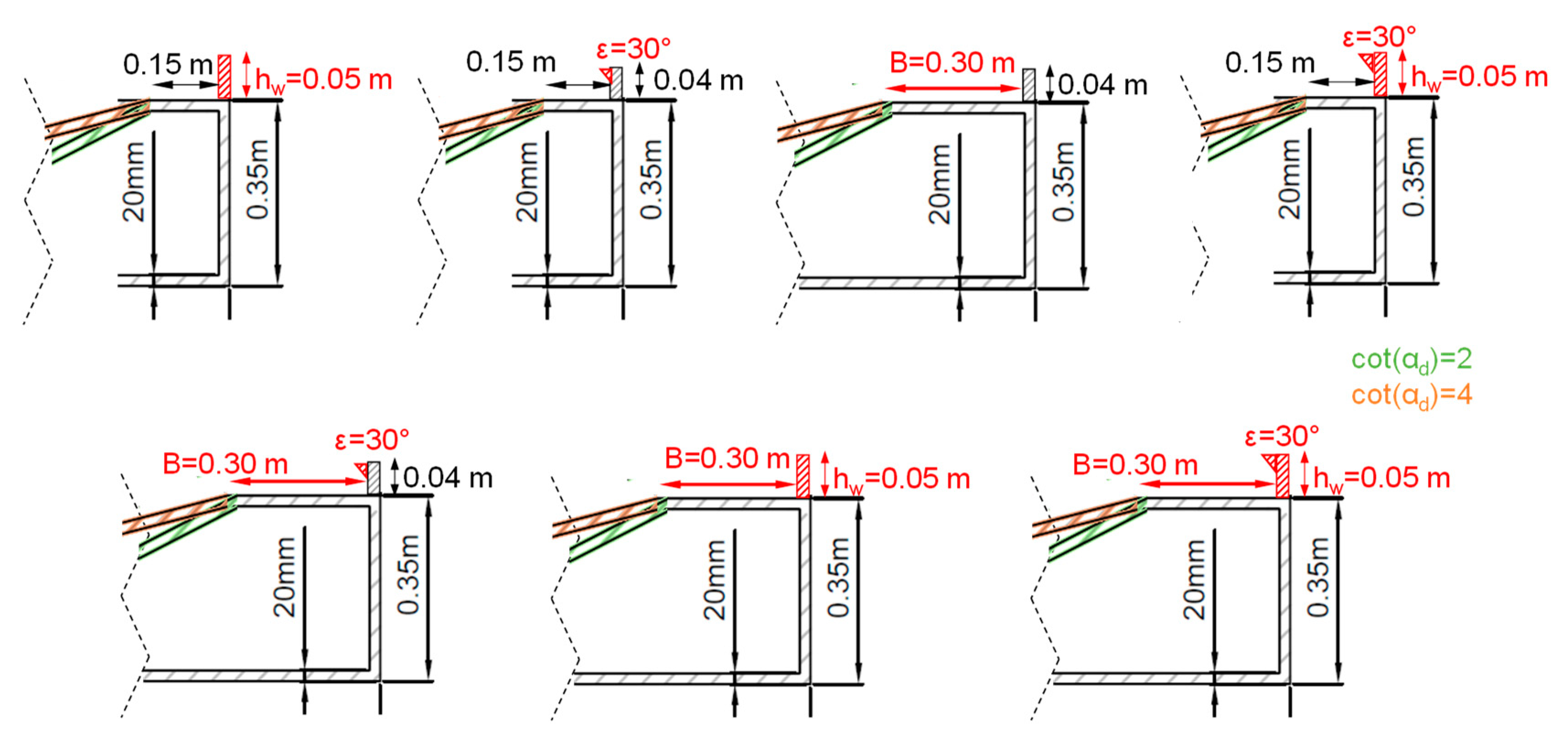
• Extension of the wall height h_w from 0.04 m to 0.05 m; this upgrade is denoted as “h_w” in the following charts and tables;
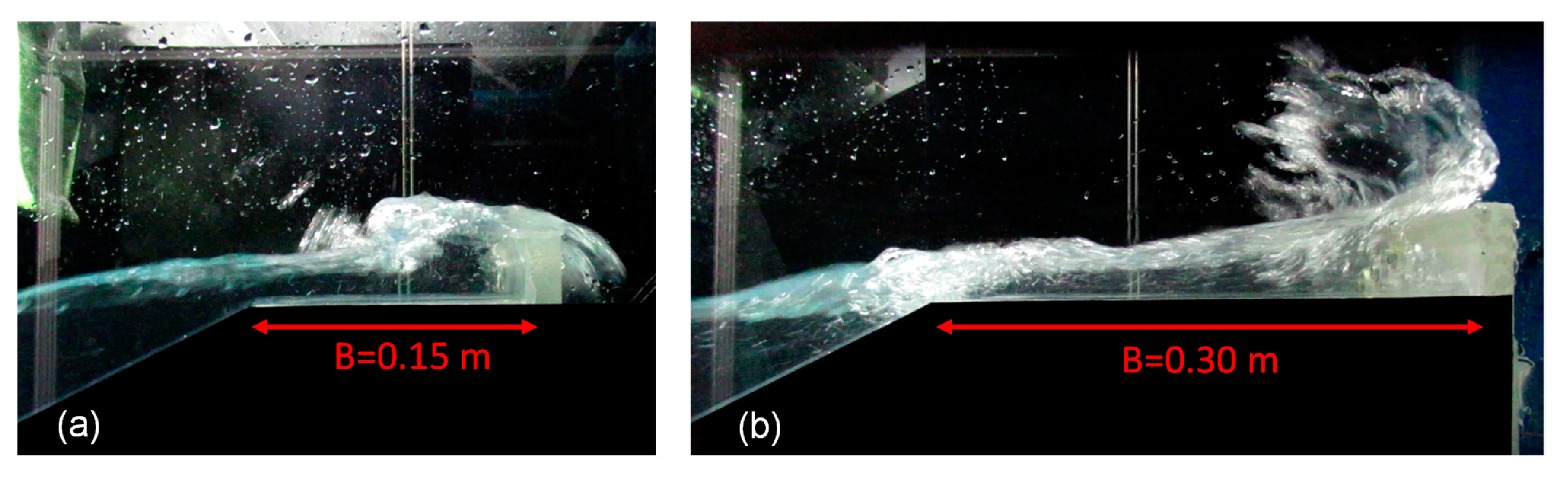
• Extension of the berm width B from 0.15 to 0.30 m (denoted as “B”);
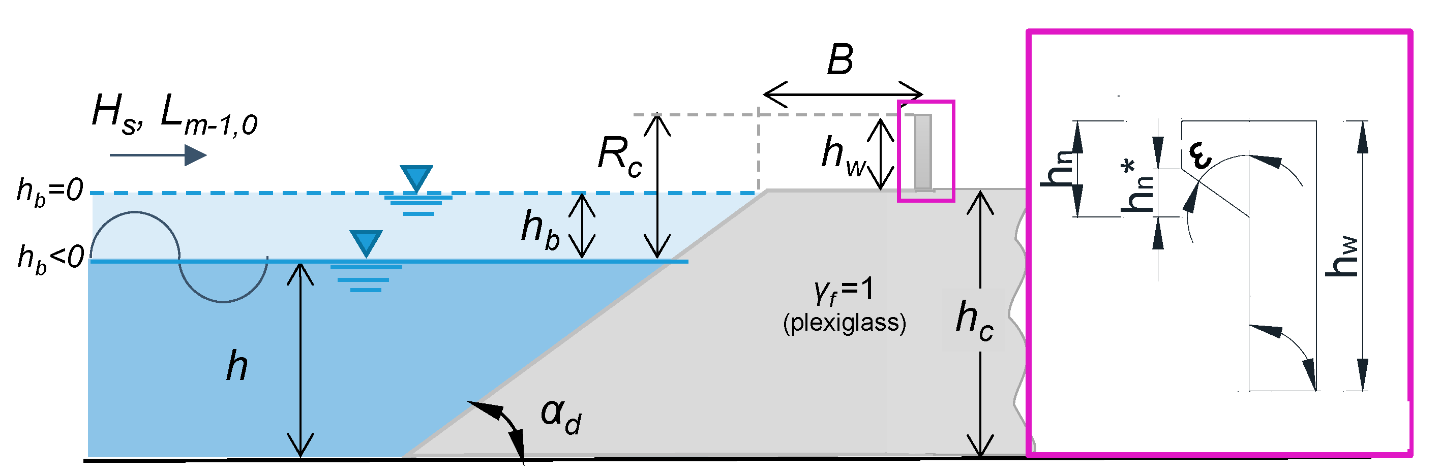
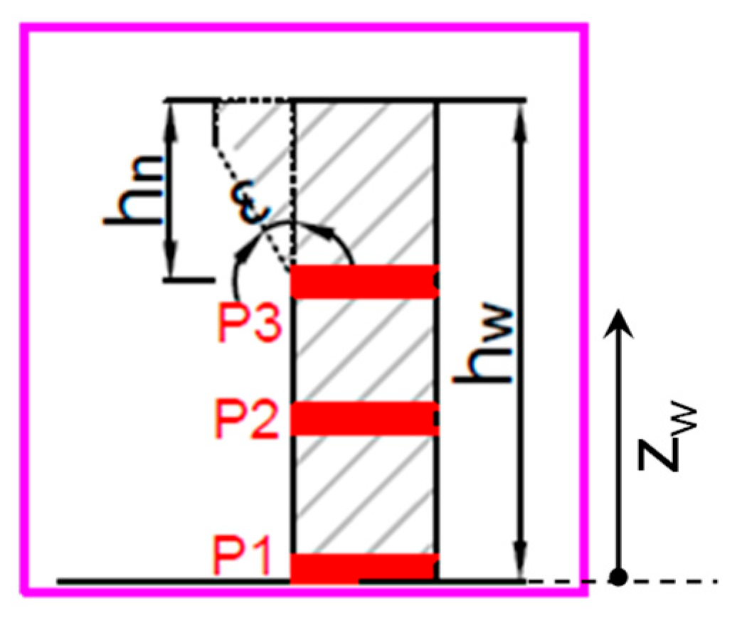
• Inclusion of a sloping parapet on top of the crown wall (upgrade “ε”); the parapet was characterized by an inclination angle of ε = 30° and a relative height λ = h_n/h_w = 0.375, where h_n is the parapet height (see Figure 1);
• Extension of h_w and contemporary inclusion of the parapet (upgrade “h_w + ε”);
• Simultaneous extension of h_w and B (upgrade “h_w + B”);
• Widening of B and simultaneous inclusion of the parapet (upgrade “B + ε”);
• Simultaneous extension of h_w, widening of B, and inclusion of the parapet (upgrade “h_w+B+ε”).

The sketches of the seven upgrades are illustrated in Figure 3.

Each combination of upgrades was installed on each of the 4 basic configurations, for a total of 32 different structures. Each configuration was subjected to four wave attacks, achieved by varying H_s (0.05 and 0.06 m) and the spectral wave periods (T_m-1,0) to obtain two target wave steepnesses (s_m-1,0 = 0.03 and 0.04). Overall, 128 experiments were therefore performed, obtaining values of the Iribarren–Battjes breaker parameter ξ_m-1,0 = tan(α_d)/(s_m-10)^0.5 varying between 1.23 and 4.00.

Table 1. Summary of the target conditions of the 128 experiments grouped by h_b/H_s.

Parameters	Configurations with hb/Hs = 0	Configurations with: hb/Hs = 0.5
Hs (m)	0.05; 0.06	0.05; 0.06
sm-1,0 (-)	0.03; 0.04	0.03; 0.04
cot(αd) (-)	2; 4	2; 4
B (-)	0.15; 0.30	0.15; 0.30
hw (-)	0.04; 0.05	0.04; 0.05
parapet (ε, λ)	no; yes (30°, 0.375)	no; yes (30°, 0.375)
#	64	64

summarizes the tested configurations, by grouping the tests by the two values of h_b/H_s = 0 and = −0.5.

While the tested conditions do correspond to mild, frequent waves in the Mediterranean Sea, and are therefore far from the typical berm design conditions, they nevertheless allow for a systematic parametric investigation of the structural and hydraulic responses of the abovementioned geometrical upgrades under the abovementioned increased wave loads.

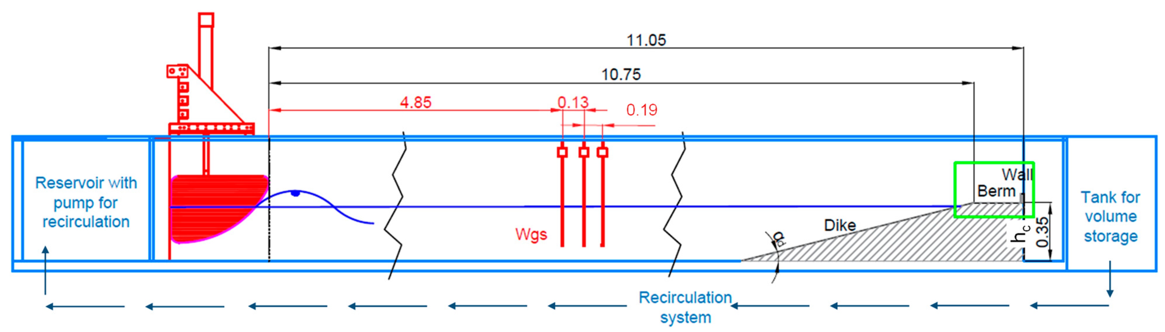
2.2. Laboratory Measurements

The wave overtopping tests were performed by collecting the overtopping volumes in a tank located behind the dike structures (see Figure 4), and by reintroducing the missing volumes in the channel through a recirculation system regulated by a flowmeter, a pump, and a hydrometer for the control of the water levels generated. The measurements of the average overtopping discharge q were derived using the flowmeter, with a precision of 1 × 10⁵ m³/(sm), and checked by measuring the total overtopping volumes in the volume storage tank.

The estimations of the instantaneous hydrodynamic forces at the crown walls, F, were obtained via the integration of the measurements of the wave pressures from three pressure transducers (P1, P2, and P3) installed along the crown wall. The positions of P1, P2, and P3, which were kept the same for all of the tests, are shown in Figure 5. The sampling frequency of the transducers was set to 1 kHz, with an accuracy of ±0.04% of the full scale, a range of measurement from 70 to 700 mbar, and a sensitive part of 3 mm for the measurement of the pressures.

For the assessment of the structural performance against the design purpose, among the several statistics extracted from the time records of the wave pressures and forces (maximum; mean; quantiles 100, 250, and 1000) and reported in Formentin et al. [28], the sole quantile F₂₅₀ was considered in this work. F₂₅₀ was estimated as the average of the N/250 impact events, where N is the number of waves of the tested time series and was adopted as design parameter by Goda [29] in preference to the maximum force, which is a more scattered parameter [30,31].

To avoid scale factors, all of the analyses were carried out and will be presented hereafter by considering the dimensionless quantities q/(gH_sT_m-1,0) and F₂₅₀/ρgR_c², where H_s, T_m-1,0, and R_c refer to the values measured in the lab. The groups of parameters chosen to make dimensionless q and F₂₅₀ follow well-established methods from the literature. The variations in R_c (included in the ±3 mm) are the consequence of the variation in the still water level in the channel. The methodology adopted to reconstruct the measured values of H_s, T_m-1,0, and R_c is detailed in [25]. Further details and explanation of the measurements, the laboratory equipment, the scale and model effects, the elaboration and filtration of the pressure signals, and the definition of the eigenfrequencies of the pressure transducers and of the crown walls are given in [28]. Issues related to the air entrainment and connected effects were investigated by Palma et al. [32].

2.3. Characterization of the New Data

The data of the average wave overtopping discharge q collected at Unibo are shown in Figure 6 in comparison to the literature data and formulae; in this figure, the data are distinguished into non-breaking (panel a) and breaking waves (panel b), according to the values of ξ_m-1,0 measured in the channel. In both of the panels, the Unibo data are plotted as red triangles against the literature data, which are shown in grey scale colors. The literature data of Figure 6a correspond to the tests by Formentin and Zanuttigh [15]. The literature data of Figure 6b represent various model tests at small and large scale carried out in 2D and 3D wave conditions and, in contrast to [15], do not strictly refer to smooth structures with crown walls, but include various datasets on breaking waves sourced from private communications and part of the original database from the CLASH (Crest Level Assessment of Coastal Structures by Full-scale Monitoring, Neural Network Prediction and Hazard Analysis on Permissible Wave Overtopping) project [33].

In both panels of Figure 6, the q-data are shown as dimensionless quantities (ordinates) as functions of the relative freeboard R_c/H_s (abscissas). The continuous and dotted curves of Figure 6 represent the mean and the 95% confidence intervals, respectively, relative to the literature formulae adopted for reference:

• The equation by Van Doorslaer et al. [14] for the non-breaking waves (panel a);
• The equation developed by Formentin and Zanuttigh [15] on the basis of the experiments carried out at Unibo and other numerical tests on wave overtopping for the breaking waves (panel b).

To the author’s knowledge, the database [14], the 128 experiments carried out at Unibo, and the numerical dataset presented in [15] represent the only data on wave overtopping at smooth dikes with crown walls and parapets available from the literature. Similarly, the abovementioned formulae are the most recent and updated formulae for the prediction of q in relation to such structures.

In both panels of Figure 6, the Unibo experiments follow the same trend as the literature data against the relative freeboard R_c/H_s, and are in good agreement with the predictive formulae. No evident model or scale effect was detected (more details about this topic can be found in [15,25]). The Unibo dimensionless data of q are collocated amongst the higher values of the q-distributions, ranging between 5 × 10⁻⁴ and 10⁻², and between 10⁻⁴ and 5 × 10⁻³, in case of non-breaking and breaking waves, respectively. Further comments and details about the Unibo q data are given in [25].

The data on the total horizontal wave forces F obtained from the integration of the pressure signals at the walls are here classified following the methodology proposed by Oumeraci et al. [34] and adopted by the project PROVERBS (Probabilistic Design Tools for Vertical Breakwaters). This classification, which is based on the nature of the wave impacts, includes four different cases:

(i)

Slightly breaking waves;

(ii)

Impact loads;

(iii)

Broken waves;

(iv)

Quasi-standing waves.

Each of these wave impacts determines the characteristic “church spire” shape of the pressure (or force) signal in the time domain, where the main peak (p_max or F_max) is followed by a trace of the duration of ~10² ms, including a second, lower peak referred to as “quasi-hydrostatic” (p_h,q or F_h,q). The PROVERBS project individuated a specific range of values of the ratio p_max/p_h,q characteristic of each breaker type: the highest values of p_max/p_h,q > 2.5 are associated with the impact loads, the slightly breaking waves are in the interval 1 < p_max/p_h,q < 2.5, while for the broken and the quasi-standing waves p_max/p_h,q ≈ 1.

For the tests carried at Unibo, the slightly breaking waves were the most recurrent wave impact types, observed in 80–85% of cases, according to the tested conditions, followed by the broken waves (5–10%) and the impact loads (3–7%).

The data of the wave forces were compared to the available literature formulae and data:

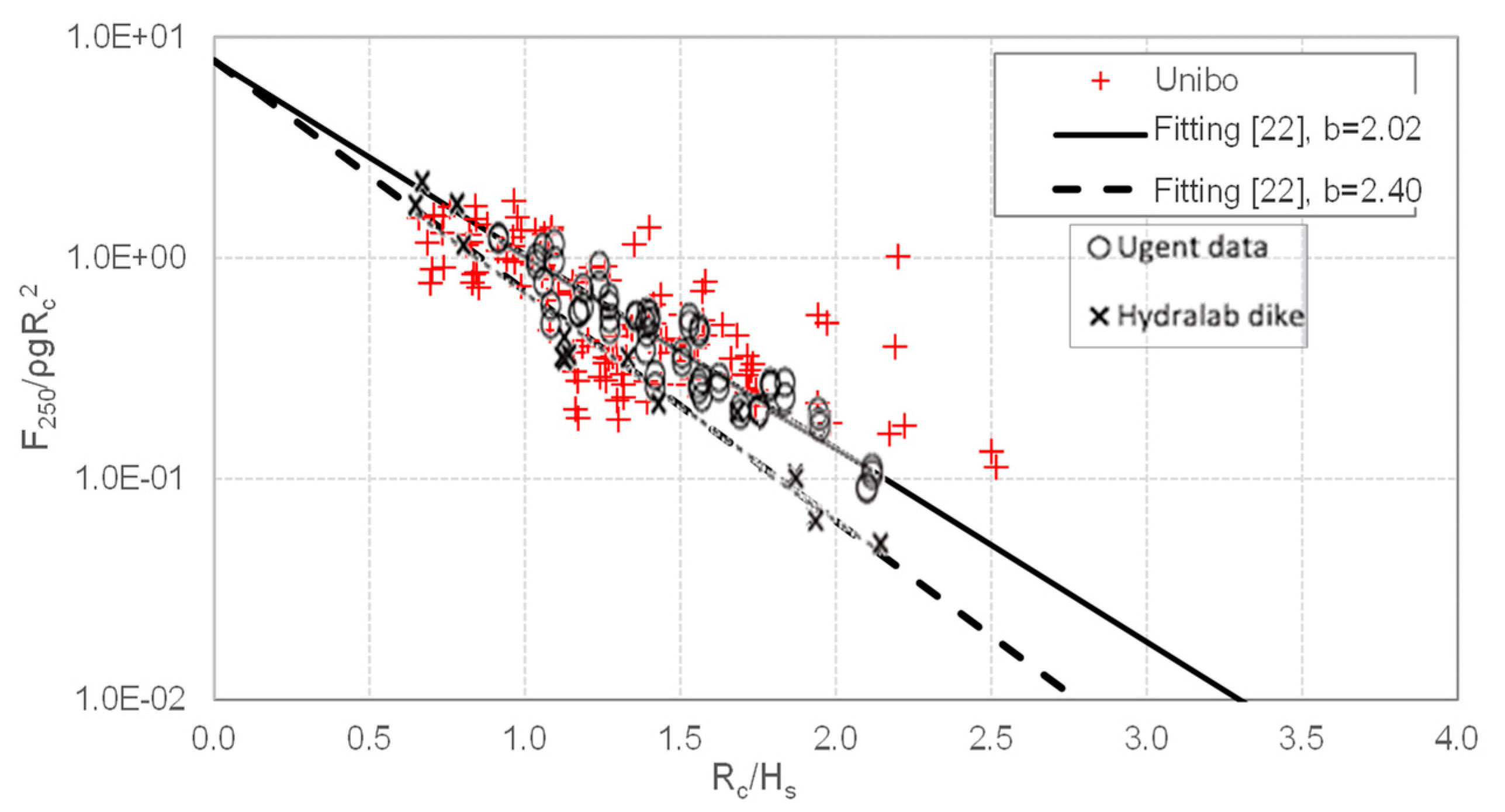
• The first design formula for predicting the wave forces on a smooth dike crown wall under irregular, non-breaking waves by Van Doorslaer et al. [31]. This formula was developed based on two sets of experiments on dikes with sloping promenades and crown walls, without parapets, carried out at different scales in the wave flume at Ghent University (“UGent data” in Figure 7 and Figure 8) and in the CIEM (Canal d’Investigació i Experimentació Marítima) wave flume of the Universitat Polytecnica de Barcelona in the context of the Hydralab project (“Hydralab data” in Figure 7 and Figure 8). The two sets of experiments were carried out at different scales, so the formula consists of two different fittings, accordingly;
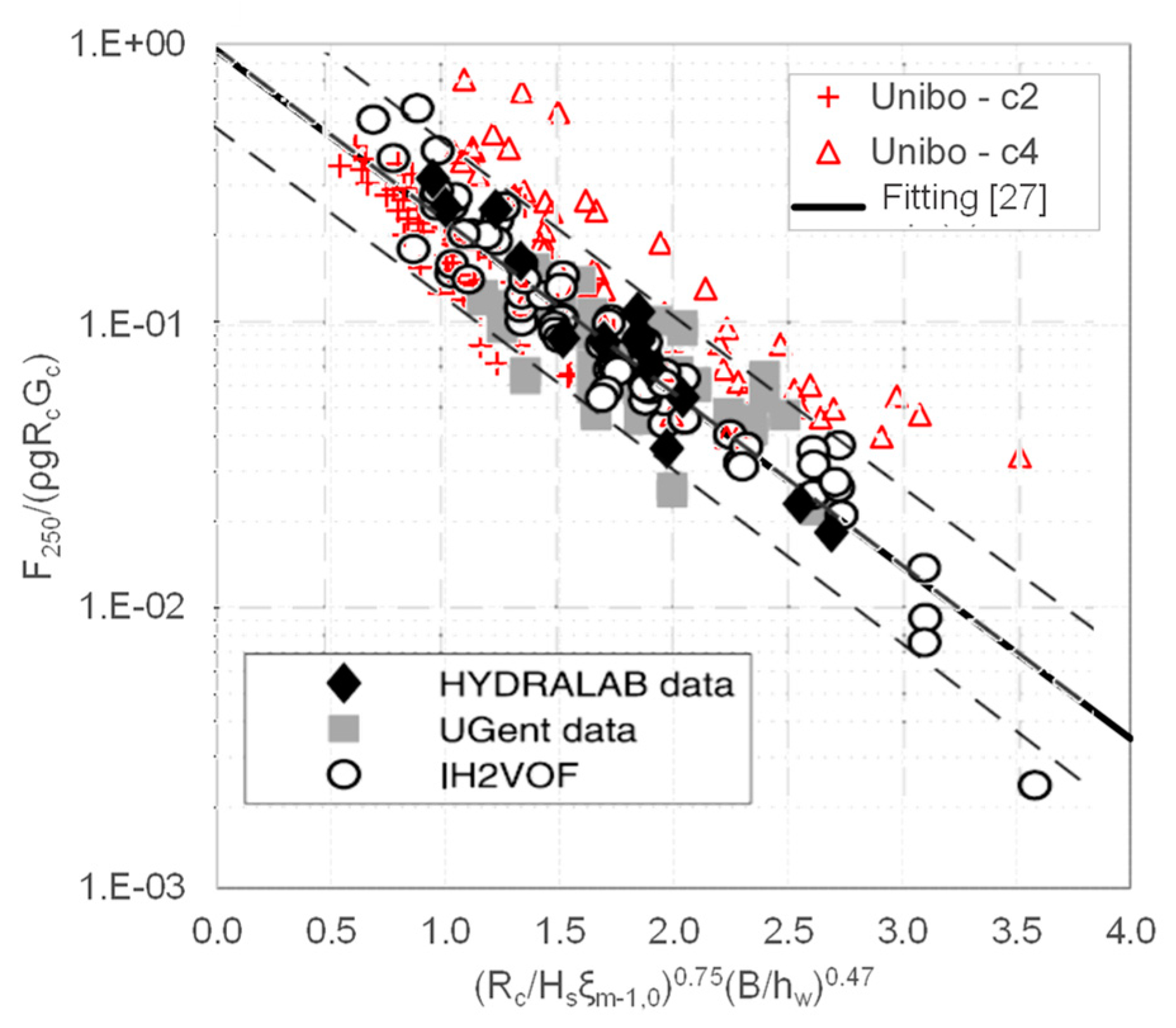
• The latest formula by De Finis et al. [35], developed on the basis of numerical simulations carried out with the IH2VOF code (developed by the University of Cantabria) to explicitly extend the Hydralab dataset with various promenade lengths and wall heights and breaking waves (“IH2VOF” in Figure 8). This formula refits the previous [31], including the parameters ξ_m-1,0, B and h_w.

Both of these formulae were calibrated on structural configurations without parapets or bullnoses.

Figure 7 and Figure 8 show the comparison between the Unibo data and the equations by [31] and [35], respectively, and with the datasets UGent, Hydralab, and IH2VOF (the information for this latter dataset was available only for Figure 8). In both Figure 7 and Figure 8, the literature data and the background charts are directly reported as in the original works, and in each of these figures the ordinate represents the F₂₅₀-values while the abscissa represents the relative freeboard R_c/H_s. Different groups of parameters were included to match the different formulations.

Figure 7 shows that most of the Unibo data are distributed around the curves representing the two fitting curves by [31], and fall in the same range as the UGent and Hydralab datasets. 8 data are significantly underestimated by the formulae: all of these points correspond to tests against structure configurations including a parapet. The underestimation of these values could be also explained with the smaller scale characterizing the Unibo data (1:20). For more details, see [28].

In Figure 8, which also reports the 95% confidence intervals associated with [35], the Unibo data are grouped by values of cot(α_d) = 2 and 4. In this figure, the scatter associated with the Unibo data is significantly reduced; however, a sharp effect of the slope is detected: almost all of the data with cot(α_d) = 4 (triangles) are underestimated by the formula. Recently, [25] proposed a refitting of this formula based on the experiments at Unibo to account for the presence of a parapet as well, and to provide a better representation of the dike slope α_d. This refitting overcomes the underestimation bias of the Unibo data with cot(α_d) = 4, while maintaining almost the same representation of the other datasets (UGent, Hydralab, and IH2VOF). The comparison with this latter refitting by [25] is not shown here, as it was calibrated against the Unibo data themselves.

3. Integrated Analysis

3.1. Effectiveness of the Structural Upgrades

The new collected data were analyzed to investigate the efficiency of each structural upgrade in achieving a reduction in q and F₂₅₀, starting from the benchmark case of the basic configuration with no upgrades, i.e., B = 0.15 m, h_w = 0.04 m, ε = 0°. The reduction in q or F₂₅₀ obtained for each configuration including one of the seven combinations of structural upgrades with respect to the basic configuration was estimated by means of the following parameter:

Red = (A_upgraded − A_basic)/A_basic

(1)

where A_basic and A_upgraded represent alternatively the values of q/(gH_m0T_m-1,0) (q*, hereafter) or of F₂₅₀/ρgR_c² (F*, hereafter) corresponding to the configuration without and including one of the mentioned structural upgrades, respectively. The values of Red were calculated for each pair of tests carried out against the same basic configuration (same h_b/H_s and same cot(α_d)) under the same wave conditions (H_s and s_m-1,0), with and without one of the seven combinations of upgrades. As example case,

Table 2. Values of Red (q*) and Red (F*) for an example case: basic configuration c2h_b0 with and without the upgrade h_w.

Configuration	Test Wave Conditions	q* [-]	Red (q*)	F*250	Red (F*)
Basic	Hs = 0.05 m, sm-1,0 = 0.03	3.34 × 10−4	-	1.56	-
Basic	Hs = 0.05 m, sm-1,0 = 0.04	2.72 × 10−4	-	1.17	-
Basic	Hs = 0.06 m, sm-1,0 = 0.03	7.32 × 10−4	-	1.01	-
Basic	Hs = 0.06 m, sm-1,0 = 0.04	5.48 × 10−4	-	1.52	-
Upgrade hw	Hs = 0.05 m, sm-1,0 = 0.03	1.79 × 10−4	−0.46	0.81	−0.48
Upgrade hw	Hs = 0.05 m, sm-1,0 = 0.04	1.21 × 10−4	−0.56	0.83	−0.29
Upgrade hw	Hs = 0.06 m, sm-1,0 = 0.03	4.84 × 10−4	−0.34	1.24	0.23
Upgrade hw	Hs = 0.06 m, sm-1,0 = 0.04	2.74 × 10−4	−0.50	1.44	−0.05
μ	-		−0.46		−0.15
σ	-		0.09		0.31

reports the individual results of q* and F*, and the related Red-factors, obtained for all four of the tested conditions with H_s = 0.05 and 0.06 m and s_m-1,0 = 0.03 and 0.04, for the basic configuration c2h_b0 with and without upgrade h_w. In this example, the average Red (q*) and Red (F*)-values and the corresponding standard deviations were calculated and reported in the last two rows of Table 2 as “μ” and “σ”, respectively.

To simplify the analysis, the average values of Red relative to the four pairs of tests with the same basic configurations and different H_s and s_m-1,0-values were considered here. In this way, the interpretation of the results can be simplified to the analysis of the four (instead of 16) groups of tests representing the four basic configurations c2h_b0, c2h_b05, c4h_b0, and c4h_b05. The variability of the Red-values is addressed in Section 5.1.3.

Figure 9 and Figure 10 show the average values of Red (q*) and Red (F*), respectively, for each of the four groups of tests.

The analysis of Figure 9 and Figure 10 leads to the following considerations, which are divided below into hydraulic and structural.

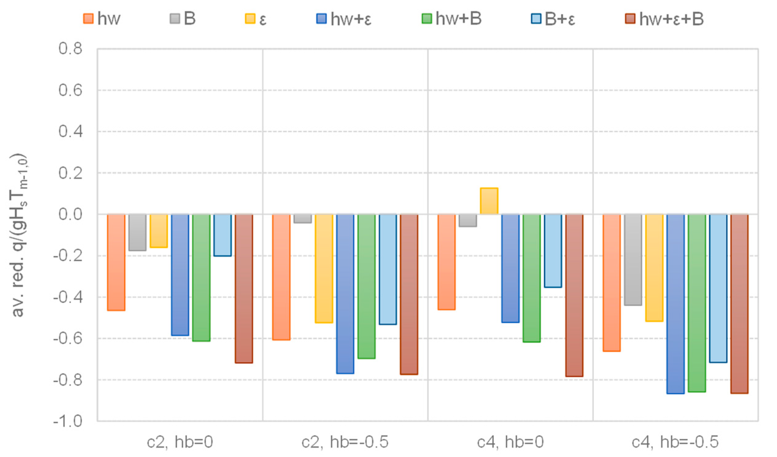
3.1.1. Hydraulic Performance

With the exception of one case (c4h_b0 = 0, upgrade “ε”), all of the structural upgrades give Red < 0, i.e., they all determine an effective reduction in q*. In most cases, the reduction was at least 20% (Red < −0.2), and frequently it was greater than 60% (Red < −0.6).

The different combinations of structural upgrades present similar overall effectiveness in reducing q* in the case of an emerged berm (h_b/H_s = −0.5), where Red varies between ≈−0.55 for the upgrade ε and ≈−0.8 for the upgrades h_w+ε, h_w+B, and h_w+ε+B. A higher variability is found in the case of h_b/H_s = 0, where Red ranges between ≈−0.2 and ≈−0.75 for the upgrades B and h_w + ε + B, respectively. This is probably due to an enhanced effect of the interaction between the incident waves and the berm when h_b/H_s = 0, leading to a higher variability in the run-up process and, consequently, in the overtopping. Therefore, in a sea level rise scenario where the berm crest is expected to work under partially submerged conditions, the effectiveness of any structural upgrade seems to be less constant and, therefore, less reliable.

For both berm conditions (h_b/H_s = −0.5 and 0), the most hydraulically effective upgrade is unquestionably h_w, determining for all the groups of tests the highest reductions in q* both when included individually (Red ≈ [−0.65; −0.5]) or in combination with B and/or ε (Red ≈ [−0.85; −0.6]). The higher efficiency of h_w could be easily predicted, as increasing h_w means increasing the total freeboard R_c. Nevertheless, the individual upgrades B and ε can produce non-negligible reductions in q*, up to Red ≈ −0.5 for the group of tests with c4 and h_b/H_s = −0.5. Furthermore, the inclusion of B and/or ε in combination with h_w might cause significant improvements (+20~30%) in the reduction in q*, with respect to the individual upgrade h_w. In conclusion, extending the berm/promenade width or including a parapet on top of a crown wall might represent a relatively effective alternative to the extension of the wall height.

Conversely, the simultaneous inclusion of B and ε (i.e., the upgrades B + ε and h_w + B + ε) is discouraged, as it does not lead to any significant improvement in the reduction in q* with respect to the individual upgrades of B and ε or h_w + ε and h_w + B.

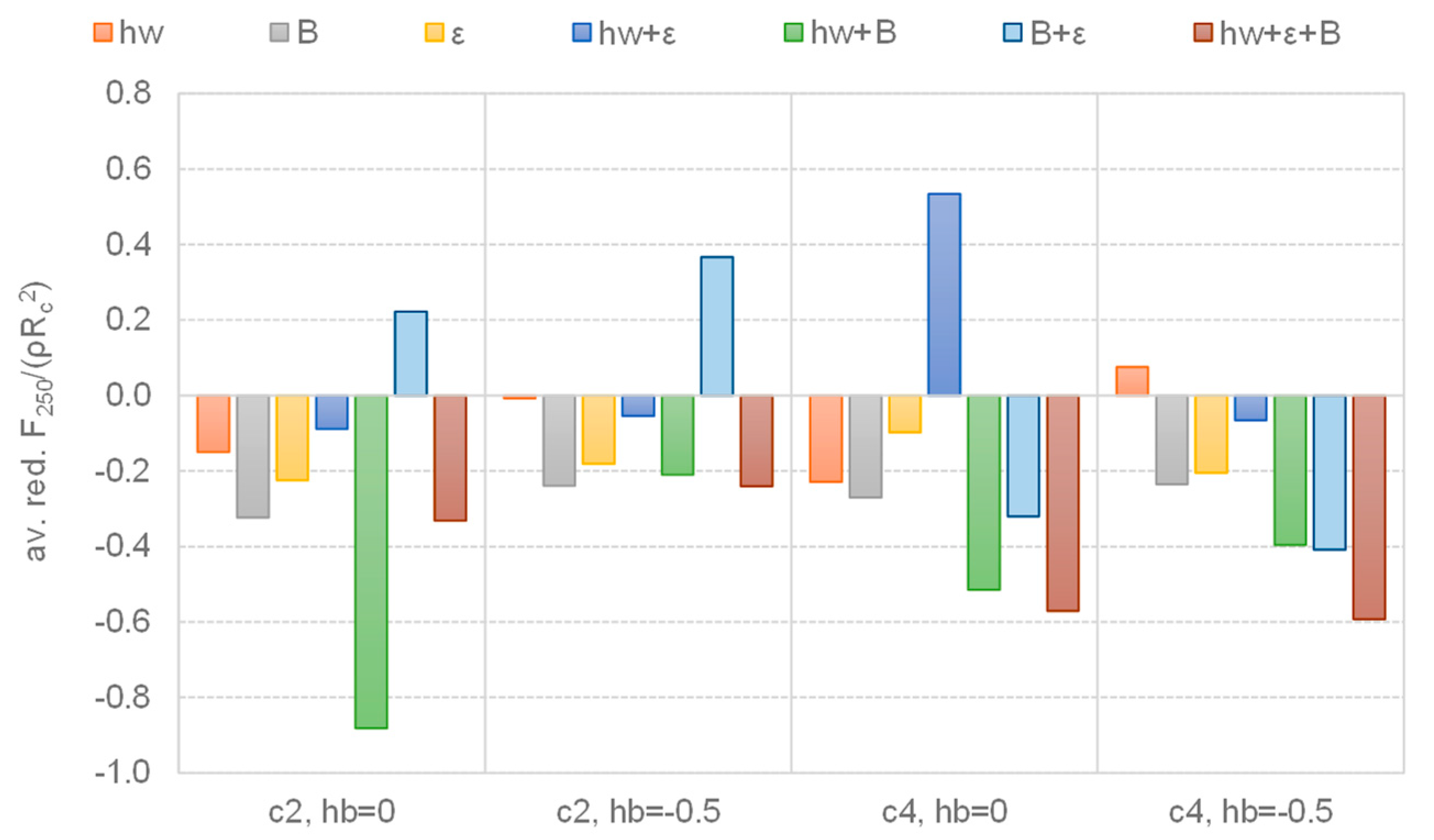
3.1.2. Structural Performance

In the chart of F*, some values of Red are positive; this means that, unlike q*, the inclusion of structural upgrades may cause increases in the wave loads. The values of Red > 0 are all associated with combinations of upgrades including ε (h_w + ε or B + ε), with the exception of one, less relevant case (upgrade h_w, group of tests c4, h_b/H_s = −0.4, Red ≈ −0.1).

When Red < 0, the reductions in F* are generally more modest than the reductions in q*, being in most cases ≈20–30% and never higher than 60% (i.e., Red < −0.6), with the exception of one case (upgrade h_w + B, group of tests c2, h_b/H_s = 0). The upgrades therefore appear more hydraulically than structurally effective.

The individual upgrade of h_w or the individual inclusion of ε determine very modest (Red > −0.2) or even negligible (Red > −0.1) reductions in F*. The individual upgrade of B seems to be more effective (Red ≈ −0.25), but the most effective combinations for the reductions in the wave forces are obtained when at least two upgrades, including the berm, are applied: h_w + B and h_w + ε + B. This result is somehow in contrast with the results associated with the reduction in q*, where the hydraulic effectiveness of an individual upgrade was substantially equivalent to the effectiveness of a combination of more upgrades.

No significant effect of h_b was observed, as similar results and considerations hold for both h_b = 0 and −0.5: the same structural performance of the upgrades is therefore expected in a sea level rise scenario.

The reductions in F* seem instead to be slightly higher in the case of c4 than in the case of c2—especially when more structural upgrades are included.

3.2. Integrated Discussion

The monotonic decreasing trends of q* and F* with R_c/H_s (see Figure 6, Figure 7 and Figure 8) would therefore suggest that the increase in the total freeboard could simultaneously ensure an effective reduction in both the wave overtopping and the total wave forces. However, when the structural upgrade consists of solutions different from the simple—but aesthetically and environmentally problematic—extension of the freeboard structure, the consequences in terms of overall performance are not as evident. The analyses presented so far in Section 3.1.1 and Section 3.1.2 indicate that combinations of upgrades that optimize the hydraulic and structural effectiveness are indeed sometimes in opposition to one another. The number of parameters involved (h_b, h_w, ε, B, cotα_d) and the different sensitivities shown by q* and F* complicate the identification of the optimal configuration for the simultaneous achievement of a satisfactory reduction in the overtopping discharge and limitation of the wave loading.

The matter is complicated even further if the sensitivity to the wave parameters—and specifically to the potential increase in the wave heights due to climate change—is also considered (see Section 5.1.3). Different wave conditions may imply different breaker types, run-up processes, and wave loading conditions for the same structure. Such differences may, in turn, generate different (opposite) responses from the hydraulic and structural points of view. For slightly breaking waves (F_max/F_h,q < 2.5), the waves go up and down the wall without rushing vertically upwards, no extreme pressure or force peaks are generated, and the formation of air pockets is limited [18]; in such conditions, the greater the run-up, the greater the overtopping at the structure’s crest, the greater the overtopping inshore of the crown wall, and the greater the force on the wall itself. On the other hand, for impact loads (F_max/F_h,q > 2.5), the waves break and overturn directly at the wall, forming large air pockets between the waves and the structure, inducing up-rushing aerated water jets and violent impacts [18], but relatively low overtopping rates. Most of the overtopping is inhibited by the overturning and the vertical up-rushing jet, which instead induce a strong wave reflection and backward flow. This phenomenon (violent impact but moderate overtopping) is further enhanced in the presence of a parapet, which confines the return flow and causes shock wave pressures [16].

Furthermore, it was found that, on average, the reduction rates Red(q*) and Red(F*) decrease with the increasing values of q* and F* themselves. Therefore, the introduction of any combination of structural upgrades is expected to be more effective—from both the hydraulic and the structural points of view—when the starting values of q* and F* (i.e., the values relative to the configurations with no upgrades) are more modest. This result is consistent with the findings of several previous studies. Among others, it is worthy to mention [10,11], recalled also in the EurOtop manual [36], highlighting that the introduction of a recurved parapet is more effective in reducing q in case of high freeboards R_c/H_s—that is to say small overtopping rates. However, whereas q is calculated behind the wall, the wave forces are calculated at the wall; this means that when an overtopping event hits and stops against the wall, giving q = 0, the wave force at the wall can be considerably >0. In conclusion, the “starting” values of q* and F* may be very different for the same configuration and, therefore, the range of the effectiveness of the structural upgrades might also be very different for q* and for F*.

In the end, the identification of the “best configuration of upgrades” to simultaneously optimize the structural and the hydraulic performance of existing dikes is not straightforward. In such a context, an efficient and simple approach to determine the “optimal configuration” of upgrades would be helpful for the purpose of design.

3.3. Costs and Environmental Impact

The optimization of engineering in the preliminary design phase always takes into account economic and environmental issues as well. To complete the integrated analysis of the performance of the various solutions, the costs and the environmental impacts associated with each of the upgraded configurations were estimated.

The costs are directly related to the volume of materials necessary to upgrade the basic structures. In this case, the structure is supposed to be made entirely of concrete. For each of the upgraded configurations, the extra volume (ΔV) was analytically calculated considering the size of the upgrades. For example, for the upgrade “B”, ΔV is given by the berm width extension (0.15 m) multiplied by the structure height h_c (0.35 m) = 0.0525 m³/m. All of the resulting ΔV-values are reported in

Table 3. Volumes, costs, and environmental impact associated with the structural upgrades. The configurations including two values of Δenv refer to the cases with h_b = 0 and h_b < 0, in that order.

Upgrade	ΔV (m3/m)	ΔV—Prototype (m3/m)	Δcost—Prototype (EUR/m)	ΔV/V (%)	Δenv. (-)
hw	2.00 × 10−4	0.08	32	0.33%	0.25 or 0.15
B	5.25 × 10−2	21.00	8400	86%	0.87 or 1.87
ε	2.25 × 10−4	0.09	36	0.37%	0.00
hw + ε	4.81 × 10−4	0.19	77	0.79%	0.26 or 0.15
hw + B	5.27 × 10−2	21.08	8432	87%	1.12 or 2.01
B + ε	5.27 × 10−2	21.08	8436	87%	0.87 or 1.87
hw + B + ε	5.30 × 10−2	21.20	8477	88%	1.13 or 2.02
Min	2.00 × 10−4	0.08	32	0.33%	0
Max	5.30 × 10−2	21.20	8477	88%	1.13 or 2.02

at the model and prototype scales, adopting a scaling factor of 20 (see Section 2).

In the Netherlands, a seawall would cost 300–500 EUR/m³ of concrete [37]. By assuming an intermediate cost of 400 EUR/m³, the extra costs (Δcost) associated with each upgrade are reported in Table 3. These costs were calculated as mere products of ΔV as the unitary cost. Possible costs specifically related to the manufacturing of the specially shaped profiles of the parapets were disregarded. Table 3 shows that the distribution of the Δcost-values is quasi-bimodal, as the upgrades h_w, ε and h_w+ε give approximately Δcost = 0, whereas all of the other upgrades including the berm give Δcost ≈ 8400 EUR/m. From this analysis, it is evident that the berm extension upgrade is the most expensive.

The environmental impact is here considered as the sum of two contributions: the ecological impact, and the aesthetic impact.

The ecological impact of maritime structures is essentially related to the following two issues [38,39]:

(i) The change in the hydro-morphodynamic regime with respect to the existing situation may affect the seabed biota and the dike colonization, and furthermore impact on the existing flora and fauna. In this case, the dike protects a harbor or the inland area and, therefore, the maintenance of the requested safety level is the project’s target, and not an impact. The offshore increase in the wave reflection from the dike due to the structural upgrade can be considered to produce minimal effects on the species colonizing the dike due to the increased wave agitation on the offshore slope. Such changes and related effects are discarded here.

(ii) The inclusion of a non-natural material, which is a hard substrate instead of a soft bottom. This effect is assumed to be a function of the extra concrete volume for the realization of the structural upgrade; it is therefore estimated as the ratio ΔV/V, where V is the volume V of the basic structure (0.06 or 24.2 m³/m at model and prototype scale, respectively). The values of ΔV/V are shown in Table 3 for each configuration.

The aesthetic impact is assumed to be directly related to the extra concrete volume, which visibly modifies the structure layout. The aesthetic impact therefore regards the vertical extension of the wall height with respect to the total freeboard R_c of the basic configuration (Δh_w/R_c = 0.25 if h_b = 0 and Δh_w/R_c = 0.15 if h_b < 0) and the horizontal extension of the berm when emerged (ΔB/B = 0 if h_b = 0 and ΔB/B = 1 if h_b < 0).

The final estimation of the environmental impact, Δenv, was calculated as the sum of ΔV/V, Δh_w/R_c, and ΔB/B, without including any weights. The values of Δenv are reported in the last column of Table 3. The configurations including two values of Δenv refer to the cases with h_b = 0 and h_b < 0, in that order.

By looking at the results of Δcost and Δenv in Table 3, it is evident that—in contrast to the effectiveness-based criteria (hydraulic and structural performance)—the analysis of the costs and of the environmental impact gives two univocal, predictable indications: the worst performance is associated with the configurations including the berm extension, while the individual introduction of the parapet represents the most performing solution. Nevertheless, as discussed in Section 3.2. the best solution according to the costs and environmental impact criteria is not necessarily the best solution from the engineering point of view.

4. Key Performance Indicators

The new methodology proposed in this paper deals with the matter of determining the “optimal configuration” to simultaneously minimize the overtopping discharge and the wave loads, limiting the costs and the environmental impact as much as possible. Bearing in mind the assumption that “there is no normative model of how individuals should make multi-criteria choices that is without critics” [40], the methodology was conceived to be as objective and as general as possible, in order to be applied independently of the specific geometries tested at Unibo. The methodology follows the approach of a simplified Multi-Criteria Analysis to define the key performance indicators (KPIs) of each configuration of structural upgrades. The criteria considered to rank the performance and calculate the KPIs are:

• The “hydraulic effectiveness” (I) and the “structural effectiveness” (II) of a configuration of structural upgrades as defined in Section 3.1. with reference to the corresponding basic configuration, and through the definition of the Red factors of Equation (1);
• The “costs” (III) and the “environmental impact” (IV) of a configuration of structural upgrades with reference to the corresponding basic configuration and based on the Δcost and the Δenv values presented in Section 3.3 and summarized in Table 2.

Scores are assigned to each upgraded configuration for each of criteria I, II, III, and IV. The KPIs of the configurations are finally computed as averages of the scores.

The criteria adopted in this study for the assignment of the scores are outlined in Section 4.1. with reference to the techniques and methods suggested in [40]. The definition of KPIs is illustrated in Section 4.2.

4.1. Scores Assignment

The following criteria were used to define and assign the Scores to the configurations of upgrades:

• Internal consistency and logical soundness;
• Ease of use;
• Ability to provide an audit trail.

For these purposes:

• All of the criteria I, II, III, and IV were weighed equally to avoid any subjectivity. The setup of weighing coefficients to reflect the relative importance of each criterion would indeed require a complicated analysis of the costs/benefits, allowing for the opinions and interests of the various stakeholders to be collected through surveys and interviews, which was beyond the scope of the present contribution;
• The scores of each criterion were calculated through simple, linear transformations of the quantities Red (criteria I and II), Δcost (III), and Δenv (IV);
• Finally, all of the Scores and the KPIs were rounded to the closest integer numbers.

As described in [40], the first requirement to set up consistent numerical scores for the assessment of the criteria is to ensure that the sense of direction is the same in all cases, so that better levels of performance lead to higher scores. It is conventional to allot a value score to each criterion between 0 and 100 or between 0 and 10 on an interval scale. In this contribution, a scale of 0–10 was adopted.

The second step consists of in establishing an interval scale for the criteria, by defining the levels of performance corresponding to the extreme scores of 0 and 10 as reference points on the scale. If possible, it is recommended to adopt a “global scaling” rule, by assigning the score of 0 to represent the worst level of performance and 10 to represent the best level. With reference to the four criteria considered in this work, the adoption of the global scaling is straightforward for criteria I and II. Indeed, for these cases, the score of 10 can be assigned to the scenario of maximum reduction in F* or q* obtained when Red = −1, and 0 can be assigned to the scenario of no reduction at all (Red = 0).

Conversely, the global scaling cannot be applied to criteria III and IV. Though the maximum score could be assigned to the configurations showing no variation in costs and no environmental impact (Δcost = 0, Δenv = 0), it is not possible to univocally assign the minimum score, as the worst scenarios of maximum costs and maximum environmental impact cannot be defined a priori. In this case, the literature suggests adopting the option of “local scaling”, associating the minimum score to the scenario that performs least well in the currently considered set of options, and the maximum score to the scenario performing best. For the criterion “costs”, the best and the worst scenarios are represented by increases in costs of 32 and 8477 EUR/m, respectively (see Table 3); for the criterion “environmental impact”, the two extreme scenarios are represented by the cases of Δenv = 0 and 2.02, respectively (see Table 3). The score 0 was therefore assigned to the scenarios with Δcost = 32 EUR/m and Δenv = 0, while the score −10 was assigned to the scenarios with Δcost = 8477 EUR /m and Δenv = 2.02. Criteria III and IV were therefore associated with negative scores, consistent with the fact that costs and environmental impact represent negative, unwanted aspects related to the upgraded configurations—as opposed to criteria (I) and (II), which represent positive effects.

The third step is represented by the definition of the scaling function. The scaling function is most commonly represented by a linear transformation of the values of the criteria to a scale of 0–10 (or −10–0). Following this approach, once fixed on a Cartesian “score–criteria” plane, with the points representing the two extreme scores assigned during the second step, the scaling functions for criteria I, II, III and IV can be derived as the linear equation fitting the two points:

$$\mathrm{Score}\left({\mathit{q}}^{*}\right)=-\mathrm{Red}\left({\mathit{q}}^{*}\right)·100,$$

(2)

$$\mathrm{Score}\left({\mathit{F}}^{*}\right)=-\mathrm{Red}\left({\mathit{F}}^{*}\right)·100$$

(3)

$$\mathrm{Score}(\Delta cos\mathit{t})=-0.48·\Delta cos\mathit{t}+0.04$$

(4)

$$\mathrm{Score}(\Delta env)=-\Delta env$$

(5)

The numerical factors −0.48 and 0.04 of Equation (4) represent the 1^st and 0^th degree coefficients, respectively, of the linear equation fitting the scores 0 and −10 associated with Δcost = 32 EUR/m and Δcost = 8477 EUR/m, respectively. The formulations (2), (3), and (5) are apparently simpler than Equation (4), because the intercepts of the fittings (0^th degree terms) are all 0 and the slopes (1st degree term) are −100 or −1, but all of the Equations (2)–(5) consistently represent the same scaling function.

Based on these scaling functions, the configurations presenting an increase in F* or q* (Red > 0) are assigned negative scores. This is consistent with the definition of the global scaling, and with the negative scores assigned to criteria III and IV. Indeed, Red >0 is an adverse, unwanted effect that negatively affects the performance of a structure, such as an increase in costs and/or environmental impact. Theoretically, Score (q*) and Score (F*) are not bottom-limited, as their values can decrease indefinitely in the event of indefinite increase in q* and F*.

Table 4. Criteria selected for the derivation of the KPIs and corresponding scoring rules.

Criterion	Scaling	Min Score	Max Score
I—Hydraulic effectiveness	Global	0, associated with Red (q*) = 0	10, associated with Red (q*) = −1
II—Structural effectiveness	Global	0, associated with Red (F*) = 0	10, associated with Red (F*) = −1
III—Costs	Local	−10, associated with Δcost = 8477 EUR/m	0, associated with Δcost = 32 EUR/m
IV—Environmental impact	Local	−10, associated with Δenv = 2.02	0, associated with Δenv = 0

reports a synthesis of the criteria and the associated scaling rules to determine the Scores.

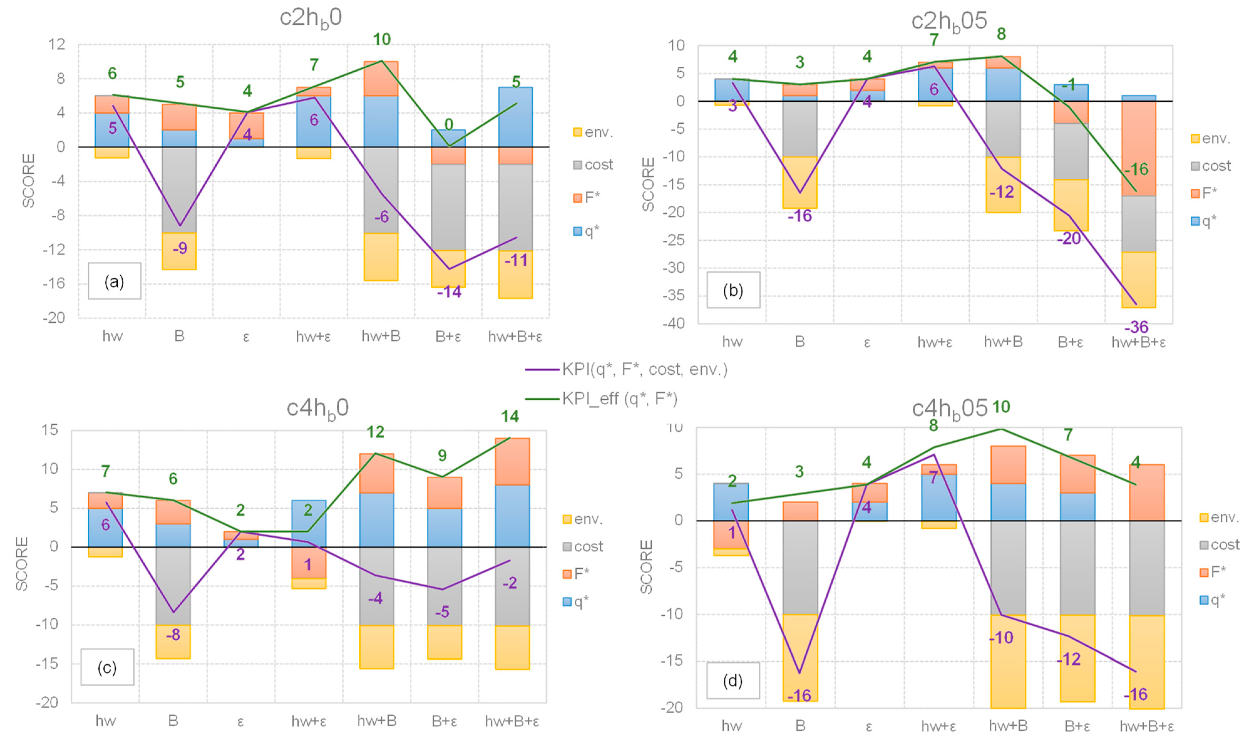
4.2. Definition of the KPIs

Most Multi-Criteria Analysis approaches use the linear additive model to calculate the final score to be assigned to a configuration [40]. The linear model shows how a configuration values for the many criteria can be combined into one overall value. This is done by adding all of the scores for each criterion together. However, this simple arithmetic sum is only appropriate if the criteria are “mutually preference independent”: it means that the preference scores assigned to all configurations for one criterion are unaffected by the preference scores for the other criteria. In other words, if it is possible to assign preference scores for the several configurations to one criterion without knowing what the configuration preference scores are for any other criteria, then this criterion is preference-independent of the others. It can be easily verified that all of the criteria—I, II, III, and IV—are mutually preference independent. Indeed, a configuration Score (q*) = 4 is preferred for criterion I to another configuration Score(q*) = 2 independently of the score ranking of all of the other criteria.

Therefore, the linear additive model was adopted to calculate the KPIs as final, overall scores to rank the performance of the different configurations:

KPI(q* + F* + Δcost + Δenv) = Score(q*) + Score(F*) + Score(Δcost) + Score(Δenv)

(6)

In order to simplify the interpretation of the results, the single Score values were rounded to the closest integer number before undergoing the sum and calculating the KPIs.

Based on the definition of Equation (6), the KPIs are integer numbers that may vary between −∞ and +40, where the upper limit is associated with the ideal scenario of Score (q*) + Score (F*) + Score (Δcost) + Score (Δenv) = 10. In practice, the KPI-values were observed to vary between –36 and 7 for the tests at Unibo.

When a configuration scores a value of KPI > 0, it means that the benefits associated to that configuration outweigh the costs. Conversely, when KPI < 0, the costs overall outweigh the benefits. Generally speaking, the configurations with KPI < 0 should not be recommended. However, a negative KPI does not directly imply that the configuration is ineffective in reducing q* and/or F*—it might be effective but expensive and/or environmentally detrimental. To highlight this aspect and differentiate the structural and hydraulic performance of a configuration from the other criteria, the following restricted indicator was also defined:

KPI_eff(q* + F*) = Score(q*) + Score(F*)

(7)

By the definition of Equation (7), KPI_eff may range between −∞ and +20. For the Unibo data, KPI_eff varied between −16 and 14. The configurations scoring:

• KPI_eff < 0 are globally ineffective and counterproductive, because the increases associated with F* and/or q* are overall greater than the reductions. These configurations are therefore strongly not recommended;
• KPI_eff = 0 are globally ineffective; this case may be due to two different causes: (1) the reduction in q* (or F*) is counterbalanced by an increase in F* (or q*); (2) the reductions in both q* and F* are 0. In both cases, these configurations are not recommended because they are useless in terms of reducing q* and F*;
• KPI_eff > 0 are globally effective and, therefore, recommendable depending on the end-user’s judgement of the corresponding KPI values.

KPI_eff is not meant to replace KPI, but to provide coastal engineers and harbor designers—as potential end-users of the proposed methodology—with a further element of evaluation of a design solution.

Table 5. Combinations of KPI and KPI_eff values, and corresponding interpretations.

KPI	KPIeff	Benefits/Costs	Configuration Effectiveness Based on Criteria I and II	Instruction
>0	>0	>1	Effective	Recommended
>0	=0	>1	Ineffective	Not recommended
>0	<0	>1	Counterproductive	Not recommended
=0	>0	1	Effective	Recommended
=0	=0	1	Ineffective	Not recommended
=0	<0	1	Counterproductive	Not recommended
<0	>0	<1	Effective	Neutral
<0	=0	<1	Ineffective	Not recommended
<0	<0	<1	Counterproductive	Not recommended

provides a summary of the possible combinations of KPI and KPI_eff-values that may result from the methodology, and the corresponding instructions that could be delivered. The ensemble of KPI and KPI_eff prompts a quantitative indication of the integrated performance of each upgraded configuration, allowing for the direct comparison of different configurations and differentiated criteria to inform a decision.

5. Application of the KPIs

5.1. Application to the Unibo Dataset

Table A1. Average values of Red (q*), Red (F*), Δcost, Δenv, relative scores, KPI, and KPI_eff obtained for the seven combinations of structural upgrades with respect to the corresponding “basic” configuration with no upgrade.

Group of Structures with Basic Configuration c2hb0
Upgrade	Red(q*) (-)	Red(F*) (-)	Δcost (EUR/m2)	Δenv (-)	Score (q*) (-)	Score (F*) (-)	Score (Δcost) (-)	Score (Δenv) (-)	KPIeff (q*, F*) (-)	KPI (q*,F*, Δcost, Δenv) (-)
hw	−0.46	−0.15	32.00	0.25	4	2		−1	6	5
B	−0.17	−0.35	8400	0.25	2	3	−10	−4	5	−9
ε	−0.14	−0.25	36.00	0.87	1	3	0	0	4	4
hw + ε	−0.57	−0.12	77.00	0.00	6	1	0	−1	7	6
hw + B	−0.60	−0.44	8432	0.26	6	4	−10	−6	10	−6
B + ε	−0.22	0.17	8436	1.12	2	−2	−10	−4	0	−14
hw + B + ε	−0.71	0.21	8477	0.87	7	−2	−10	−6	5	−11
Min	−0.71	−0.44	0.00	0.00	1	−2	−10	−6	0	−14
Max	0.00	0.21	8477	1.13	7	4	0	0	10	6
μ	−0.36	−0.12	4239	0.56	4.00	1.29	−5.77	−3.17	5.29	−3.65
Group of Structures with Basic Configuration c2hb05
Upgrade	Red(q*) (-)	Red(F*) (-)	Δcost (EUR/m2)	Δenv (-)	Score (q*) (-)	Score (F*) (-)	Score (Δcost) (-)	Score (Δenv) (-)	KPIeff (q*, F*) (-)	KPI (q*,F*, Δcost, Δenv) (-)
hw	−0.39	−0.01	32.00	0.25	4	0	0	−1	4	3
B	−0.09	−0.25	8400	0.15	1	2	−10	−9	3	−16
ε	−0.24	−0.18	36.00	1.87	2	2	0	0	4	4
hw + ε	−0.62	−0.06	77.00	0.00	6	1	0	−1	7	6
hw + B	−0.57	−0.22	8432	0.15	6	2	−10	−10	8	−12
B + ε	−0.31	0.36	8436	2.01	3	−4	−10	−9	−1	−20
hw + B + ε	−0.09	1.65	8477	1.87	1	−17	−10	−10	−16	−36
Min	−0.62	−0.25	0.00	0.00	1	−17	−10	−10	−16	−36
Max	0.00	1.65	8477	2.01	6	2	0	0	8	6
μ	−0.29	0.16	4239	0.90	3.29	−2.00	−5.77	−5.69	1.29	−10.17
Group of Structures with Basic Configuration c4hb0
Upgrade	Red(q*) (-)	Red(F*) (-)	Δcost (EUR/m2)	Δenv (-)	Score (q*) (-)	Score (F*) (-)	Score (Δcost) (-)	Score (Δenv) (-)	KPIeff (q*, F*) (-)	KPI (q*,F*, Δcost, Δenv) (-)
hw	−0.52	−0.22	32.00	0.25	5	2	0	−1	7	6
B	−0.28	−0.29	8400	0.25	3	3	−10	−4	6	−8
ε	−0.06	−0.12	36.00	0.87	1	1	0	0	2	2
hw + ε	−0.59	0.40	77.00	0.00	6	−4	0	−1	2	1
hw + B	−0.72	−0.52	8432	0.26	7	5	−10	−6	12	−4
B + ε	−0.46	−0.36	8436	1.12	5	4	−10	−4	9	−5
hw + B + ε	−0.79	−0.58	8477	0.87	8	6	−10	−6	14	−2
Min	−0.79	−0.58	0.00	0.00	1	−4	−10	−6	2	−8
Max	0.00	0.40	8477	1.13	8	6	0	0	14	6
μ	−0.43	−0.21	4239	0.56	5.00	2.43	−5.77	−3.17	7.43	−1.51
Group of Structures with Basic Configuration c4hb05
Upgrade	Red(q*) (-)	Red(F*) (-)	Δcost (EUR/m2)	Δenv (-)	Score (q*) (-)	Score (F*) (-)	Score (Δcost) (-)	Score (Δenv) (-)	KPIeff (q*, F*) (-)	KPI (q*,F*, Δcost, Δenv) (-)
hw	−0.46	0.32	32.00	0.25	5	−3	0	−1	2	1
B	−0.10	−0.24	8400	0.15	1	2	−10	−9	3	−16
ε	−0.20	−0.21	36.00	1.87	2	2	0	0	4	4
hw + ε	−0.67	−0.07	77.00	0.00	7	1	0	−1	8	7
hw + B	−0.63	−0.40	8432	0.15	6	4	−10	−10	10	−10
B + ε	−0.29	−0.43	8436	2.01	3	4	−10	−9	7	−12
hw + B + ε	0.17	−0.60	8477	1.87	−2	6	−10	−10	4	−16
Min	−0.67	-0.60	0.00	0.00	−2	−3	−10	−10	2	−16
Max	0.17	0.32	8477	2.01	7	6	0	0	10	7
μ	−0.27	−0.20	4239	0.90	3.14	2.29	−5.77	−5.69	5.43	−6.03

(in Appendix A) collects the results of the application of Equations (2)–(5) to the experiments carried out at Unibo; each Score, KPI, and KPI_eff value in this Ttable corresponds to the average result obtained on the sets of four different tests carried out against the same structure configuration, varying the H_s and s_m-1,0-values (H_s = 0.05 and 0.06 m, s_m-1,0 = 0.03 and 0.04). Table A1 is subdivided into four parts corresponding to the four “basic configurations” with no upgrades (the same as in Figure 8 and Figure 9): (1) c2h_b0; (2) c2h_b05; (3) c4h_b0; and (4) c4h_b05.

The stacked bar charts of Figure 11 show the average values of Score(q*), Score(F*), Score (Δcost), and Score (Δenv) calculated for each combination of upgrades. The averages of the scores were computed from the four tests carried out against the same structures under different wave attacks. The piecewise lines represent the KPI and KPI_eff values corresponding to each combination. The four panels comprising Figure 11 are relative to the four groups of tests c2h_b0, c2h_b05, c4h_b0, and c4h_b05.

5.1.1. Ranking of the Upgrades

It appears evident from Figure 11 that none of the configurations of upgrades are ever counterproductive, because KPI_eff is always >0—with the exception of B+ε and h_w+B+ε, exclusively for group c2h_b05. On the other hand, many configurations score negative KPI values, denoting an overall disadvantageous cost/benefit ratio.

The global ranking of the configurations of upgrades can be derived on the basis of the corresponding average values of the KPI computed over the four groups of tests. For example, the upgrade h_w+ε—scoring KPI = 6, 6, 1, and 7 for the groups c2h_b0, c2h_b05, c4h_b0, and c4h_b05, respectively (see Table A1 or Figure 11)—obtains an average value μ(KPI) = 5. The average μ(KPI) for each configuration is reported in

Table 6. Global ranking of the configurations of upgrades based on μ(KPI).

Ranking	Upgrade	μ(KPI)	KPI	KPIeff	Instruction
1	hw + ε	5	>0	>0	Recommended for all of the groups of structures
2	ε	4	>0	>0	Recommended for all of the groups of structures
3	hw	3.75	>0	>0	Recommended for all of the groups of structures
4	hw + B	-8	<0	>0	Neutral for all of the groups of structures
5	B	−12.25	<0	>0	Neutral for all of the groups of structures
6	B + ε	−12.75	<0	≤0 for c2, >0 for c4	Not recommended for c2; neutral for c4
7	hw + B + ε	−16.25	<0	<0 for c2hb05 >0 otherwise	Not recommended for c2hb05; neutral otherwise

; the instructions proposed in this Table follow the logic illustrated in Table 5, based on the analysis of the KPI- and KPI_eff-values.

The combination of upgrades reaching the maximum KPI values for three groups of structures out of four is h_w + ε, with KPI = 6 in the cases of c2h_b0 and c2h_b05, and KPI = 7 in the case of c4h_b05. Although this combination is outperformed by the combinations h_w (KPI = 6) and ε (KPI = 2) in the group c4h_b0, here it still presents a KPI > 0 (KPI = 1). Therefore, the combination of h_w + ε was the best performing throughout the four groups of tests.

The only two further combinations presenting positive KPI values throughout the four groups of tests are h_w (KPI = 5, 3, 6, and 1) and ε (KPI = 4, 4, 2, and 4). Thus, the individual upgrades of h_w and ε, as well as their combination h_w+ε, can always be recommended, i.e., for both breaking and non-breaking wave conditions, as well as when accounting for a future sea level rise scenario.

All of the other configurations B, h_w + B, B + ε, and h_w + B + ε systematically show negative KPIs throughout the four groups of tests. The performance of these configurations is negatively affected and compromised by their huge costs (when compared to the other configurations) and the high environmental impact caused by the presence of the berm. The analysis of the KPI_eff values allows the effectiveness of these configurations to be investigated separately from their overall performance.

The configuration h_w + B (KPI_eff = 10, 8, 12, and 10) presents on average the highest KPI_eff values throughout all of the groups of tests and, in most cases, the maximum KPI_eff values relative to each group of tests. This configuration therefore presents the maximum hydraulic and structural effectiveness—even in comparison to the abovementioned, best performing configuration h_w + ε. On the other hand, it is also the second most expensive and the most environmentally detrimental configuration—second and equal, respectively, to h_w + B + ε. This latter configuration (h_w + B + ε), including all of the upgrades, presents the absolute maximum KPI_eff = 14 for the group c4h_b0, but it scores KPI_eff = 5, −16, and 4 when applied to the groups c2h_b0, c2h_b05, and c4h_b05, respectively.

The effectiveness of the solution B + ε seems to be strongly related to the slope (and therefore the breaking/non-breaking wave conditions); this combination shows KPI_eff = 9 and 7 in the case of c4h_b0 and c4h_b05, respectively, but KPI_eff = 0 and −1 for c2h_b0 and c2h_b05, respectively. This result is peculiar because the individual upgrades B and ε seem not to present the same effects related to the slope, but rather indicate a relationship with the berm emergence (KPI_eff = 5, 3, 6, and 3 for B, and KPI_eff = 4, 4, 2, and 4 for ε, for the four groups c2h_b0, c2h_b05, c4h_b0, and c4h_b05, respectively). Figure 11a,b suggest that the low KPI values associated with B+ε in the case of c2 are principally due to the negative Scores of F* (Score(F*) = −2 and −4 for c2h_b0 and c2h_b05, respectively) rather than to the Score values of q*, which are both positive (Score(q*) = 2 and 3 for c2h_b0 and c2h_b05, respectively). Therefore, in the case of c2, the upgrade B+ε causes a reduction in the overtopping discharge at the expense of an increase in the wave loads. The higher loads—a consequence of the confined return flow caused by the parapet—are evidently enhanced by the association of the parapet with the increased berm width (see Section 3.1.2). Figure 12 displays the same overtopping event occurring at the same structure (cot(α_d) = 2, h_b/H_s = 0, h_w = 0.04 m, ε = 30°) in the case of B = 0.15 m (panel a) and of B = 0.30 m (panel b). In both of the tests, the parapet contributes to reducing the overtopping, but the dynamics of the wave impact and the amount of air entrainment are completely different—whereas the wave merely hits the wall and reflects back in panel a, it instead rushes vertically up the wall, splashing violently against it, in panel b. The slope in c4 does not cause a similar situation, as the breaking waves are far from causing such violent impacts at the wall and the consequent enhancement of the wave forces.

In contrast to B + ε, the effectiveness of the individual upgrade B is principally related to h_b/H_s. Specifically, the upgrade of B is more effective when h_b/H_s = 0, with KPI_eff = 5 and 6 for c2h_b0 and c4h_b0, respectively and KPI_eff = 3 and 3 for c2h_b05 and c4h_b05, respectively. This result can be easily predicted and explained, as the berm is more effective in reducing q* and F* if it is at the still water level and induces the wave breaking and the wave energy dissipation by interacting with the incoming waves. When h_b/H_s < 0, the waves reach the berm already broken, and the reducing effect due to the wave–berm interaction is therefore modest or null. Therefore, the increase in the berm width might represent an efficient solution in a sea level rise scenario—especially considering the fact that a berm at the still water lever does not have an aesthetic impact.

5.1.2. Optimizing the Performance of the Upgrades

The performance of the structural upgrades is better for the configurations with the slope c4 (panels a and b of Figure 11), presenting KPIs with μ = −1.51 and −6.03 for the groups c4h_b0 and c4h_b05, respectively, and lower for the configurations with c2 (panels c and d), characterized by KPIs with μ = −3.65 and −10.17 for c2h_b0 and c2h_b05, respectively. The data collected in Table A1 reveal that the criteria determining the lower performance of c2 are I and II because, for a given configuration, the values of Score(Δcost) and Score(Δenv) are the same for both c2 and c4. Figure 11 shows that all of the KPI_eff-values associated with c2 (panels a and b) are consistently equal to or lower than the corresponding values for c4 (panels c and d) for all of the combinations of upgrades. Therefore, the structural upgrades are less effective overall when non-breaking wave conditions occur (ξ_m-1,0 is always >2 in case of c2), independently of the specific configuration of upgrades (μ(KPI_eff) = 7.43 and 5.43 for c4h_b0 and c4h_b05, respectively, and μ(KPI_eff) = 5.29 and 1.29 for c2h_b0 and c2h_b05, respectively). This result can be explained by the dynamics of the wave overtopping process: the waves tend to more frequently reach the wall unbroken and impact more violently against it, leading to higher overtopping rates q* and more intense wave impacts F* with respect to the breaking wave conditions. As observed in the literature [36], the scale of the reduction in q* and/or F* is correlated with the scale of the overtopping rate and/or of the wave loads themselves; in other words, the reduction rates Red (q*) and Red (F*) are lower if q* and F* are higher, and the KPIs are more modest accordingly.

By analyzing the individual Score-values more deeply, it can be observed that the main criterion negatively affecting the performance of the configurations with c2 is the structural effectiveness (II), which is particularly low in case of the configurations B+ε (Score(F*) = –2 and –4 for c2h_b0 and c2h_b05, respectively) and h_w + B + ε (Score(F*) = –2 and –17). The non-breaking waves (c2) tend to generate impact loads at the walls, and this phenomenon is enhanced in the presence of parapets (see Section 3.1.2). The introduction of the KPIs allows the assessment of the scale of this phenomenon on the overall performance of the parapet with respect to other benefits, such as its low cost, low environmental impact, and its effectiveness in reducing q*. For example, the configurations B+ε and h_w+B+ε still present positive values of both KPI and KPI_eff for the configuration h_b0 (Figure 11a), despite the negative values of Score (F*). Therefore, the upgrades B+ε and h_w+B+ε can be still recommended in the case of c2h_b0. On the other hand, these upgrades give negative KPI- and KPI_eff-values for c2h_b05, and in this case are not recommendable.

The performance of the upgrades is also greater for configuration h_b0 (panels a and c of Figure 11) than for configuration h_b05 (panels b and d), considering both the average (μ) and the maximum values of the KPI. In this case, the criterion most negatively affecting the performance is the environmental impact (IV), showing an average Score(Δenv) = −3.17 for h_b0 and Score(Δenv) = −5.77 for h_b05. Of course, the extension of the berm (upgrades B, h_w+B, B+ε, h_w+B+ε) has a greater aesthetic impact if the berm is emerged (h_b05).

Criteria I and II also negatively affect the performance of h_b05: by comparing the average KPI_eff-values, the integrated hydraulic and structural effectiveness of the upgrades is nearly four times greater when the berm is not emerged and the slope is c2 (μ(KPI_eff) = 5.29 and 1.29 in the cases of c2h_b0 and c2h_b05, respectively) and 1.37 times higher when the slope is c4 (μ(KPI_eff) = 7.43 and 5.43 in the cases of c4h_b0 and c4h_b05, respectively). The decrease in performance related to the emerged berm level can be explained through the nature of the wave impacts. In [25], it was observed that the impact type more frequently associated with the case of h_b05 is the broken wave. Indeed, when h_b < 0, the incident waves tend to break along the slope, dissipating most of their energy in the run-up process and leading to a low-energetic bore flow above the berm and weak wave impacts at the walls. The bore flow is barely affected by the presence of any of the structural upgrades, and their effectiveness is therefore modest.

By combining the conclusions drawn thus far, the performance (KPI) and the effectiveness (KPI_eff) of the structural upgrades is optimized in the case of slightly breaking conditions, associated with the configurations c4 and h_b0, and limited for non-breaking (c2) or fully broken waves (h_b0).

5.1.3. Variability of the Results

The stacked bars of Figure 11 and the data reported in Table A1 refer to average values of Red(q*) and Red(q*) calculated over each group of four pairs of tests carried out against the same structural configuration under different wave conditions. Conversely, Table 2 shows—for the selected example case—the individual values of Red(q*) and Red(F*) obtained for each pair of tests at the variation of H_s and s_m-1,0. The variability of the results of this Table—as assessed through the calculation of the standard deviations σ—is referred to in this Section as a representative case to complete the analysis of the average Score- and KPI-values conducted so far, while also accounting for the effects of H_s and s_m-1,0. Note that the discussion of the variability of the results does not apply to criteria III and IV of the present Multi-Criteria Analysis, as the costs and the environmental impact depend exclusively on the structural layout, and do not vary with the wave attacks.

The increase in H_s from 0.05 to 0.06 m as an effect of climate change is described in detail in [28]. In short, it was found that the changes in H_s determine “pure” scale effects on both the q- and F-values, as well as on the shape of the profile of the wave pressures along the crown wall height. The term “pure” is used to denote that the variations in the q- and F-values seem not to be strictly correlated with the structural configuration or other variables aside from H_s itself. More specifically, changing H_s by +25% determines an increase in q between +28% and +415%, on average of +145%, with a standard deviation of +77%. The same change determines a variation in F₂₅₀ between −36% (i.e., reduction) and +121%, with an average of +27% and a standard deviation of +28%. Based on the Unibo experiments, a scenario of increased the wave height is thus expected to impact more on the hydraulic loads than on the structural stresses at the coastal structures.

The variability of the Red(q*) and Red(F*) values is not affected by the changes in the wave heights: the average Red(q*) calculated among all of the tested configurations subjected to wave attacks with H_s = 0.05 m was −0.55, whereas the average Red(q*) calculated for the wave attacks with H_s = 0.06 m was −0.49; similarly, the averages of Red (F*) calculated for H_s = 0.05 and 0.06 m were −0.18 and −0.23, respectively. Consequently, the variability of the Scores and of the KPIs is not dependent on the changes in H_s.

The data reported in the exemplifying case from Table 2 are consistent with these results.

To further investigate the variability of the results of the methodology proposed thus far—independently of the wave attack conditions—the “standard deviation scores” of Red_σ (q*) and Red_σ (F) are introduced as follows:

$${\mathrm{Score}}_{\mathsf{\sigma }}\left({\mathit{q}}^{*}\right){=\mathit{Red}}_{\mathsf{\sigma }}\left({\mathit{q}}^{*}\right)·100,$$

(8)

$${\mathrm{Score}}_{\mathsf{\sigma }}\left({\mathit{F}}^{*}\right){=\mathit{Red}}_{\mathsf{\sigma }}\left({\mathit{F}}^{*}\right)·100$$

(9)

These “standard deviation scores” Score_σ are obtained by replacing the average Red-values in the definitions of the Scores by Equations (2) and (3). The values of Score_σ (q*) and Score_σ (F*) are added as deviation bars of the average Score(q*) and Score(F*) values in the chart of Figure 13, where the stacked bars are directly taken from Figure 11. When the deviation bars are not visible in Figure 13, it means that the corresponding Score_σ is equal (or close) to 0.

The Score_σ (q*) and Score_σ (F*) values vary between 0 and 3 and between 0 and 5, respectively. The sum of Score_σ (q*) and Score_σ (F*) varies between 1 and 7. The average Score_σ (q*) and Score_σ (F*) are 1.71 and 1.50, respectively, the average of Score_σ (q*) + Score_σ (F*) is 3.21, while the mode of Score_σ (q*), Score_σ (F*), and Score_σ (q*) + Score_σ (F*) is 2, 1, and 2, respectively. According to the statistics of Score_σ (q*) + Score_σ (F*), it can be determined that the width of the one-standard-deviation-confidence interval associated with the average KPI and KPI_eff values varies between 1 and 7, is 3.21 on average, and in most cases it is 2.

The maximum Score_σ (F*) = 5 is associated with the individual case of the basic configuration c2h_b05 upgraded with h_w + B + ε (Figure 13c), which is also the configuration characterized by the lowest KPI and KPI_eff values. The fact that the highest variability is associated with this configuration suggests that not all of the four wave attacks may generate the same poor performance. In fact, for two tests out of four, the configuration determined a slight reduction in both q* and F*; however, the increase in F* observed for the remaining two tests was so high that the resulting average Score (F*) value negatively affected the KPI and KPI_eff. The combined analysis of average and standard deviation Scores reveals that the performance of the configuration is very “unstable”, rather than completely ineffective; however, it also cannot be recommended.

The maximum Score_σ (q*) = 3 is associated with eight different cases, corresponding to different basic configurations and different combinations of upgrades. Unlike criterion II, criterion I does not show a single outlier case characterized by a high standard deviation, but it presents a more uniformly distributed variability of the results across the several configurations.

The Score_σ deviation bars of Figure 13 and the average Score_σ (q*) and Score_σ (F*) values indicate that the variability of the performance is lower for criterion I than for criterion II. This reflects and depends on the uncertainty related to the measurements of the overtopping discharge and of the wave forces. In the latter case, the high speed of the wave impact process—especially in the case of impact loads or slightly-breaking waves—along with the aeration levels of the impinging waves and the limited size of the installation facilities, generates higher uncertainty in the measurements (see [25] for details on scale and model effects).

5.2. Application to Literature Datasets

This Section presents the results of the application of Scores and of the KPIs (Equation (6)) to experiments on wave overtopping and wave loads at walls and crown walls available from the literature. To the author’s knowledge, the only data available on simultaneous measurements of overtopping discharges and forces are from the following three studies:

• Pearson et al. [11], who collected 373 experimental data on wave overtopping and wave forces on crown walls on top of differently armored rubble mound breakwaters (rock, cube, and dolos);
• Smolka et al. [19], who carried out small-scale 2D tests against a cube- and Cubipod-armored mound breakwater, measuring the data of the dimensionless horizontal and uplift forces, and of the overturning moments at the crown wall;
• Martinelli et al. [17], who conducted regular and irregular tests of wave overtopping against a seawall with a recurved parapet whose inclination angle ε was varied between 0° and 90°. During the tests, measurements of the overtopping discharge and of the wave forces at the base of the wall were collected.

In this study, two datasets were considered for the application of the KPI methodology: one dataset named “P” from Pearson et al. [11], and one dataset named “M” from Martinelli et al. [17]. The selection of the data was intended to simplify the parametric analysis and build “homogeneous” datasets including “basic configurations” and “upgraded configurations” subjected to the same variety and approximately the same number of wave states so that the results of q*, F*, Red, etc., could be averaged consistently.

To this purpose, the dataset “P” was composed by considering only the data presenting: (1) cot(α_d) = 1.5, (2) rock-armor revetment, and (3) values of the berm emergence h_b in the range (−0.04; 0.04), for a total of 159 tests. The “basic configuration” of the dataset “P” thus includes 43 tests characterized by the same values of h_w = 0.15 m and B = 0.18, and by H_s = (0.105; 0.181) m, T_m-1,0 = (1.09; 2.00) s, and R_c/H_s = (0.61; 1.76) m. Five different upgraded configurations were then individuated: (1) extension of h_w to 0.24 m; (2) extension of h_w to 0.33 m; (3) extension of h_w to 0.24 m and widening of B to 0.24 m; (4) extension of h_w to 0.24 m and widening of B to 0.3 m; and (5) extension of h_w to 0.24 m and widening of B to 0.36 m. For each upgraded configuration, the values of H_s, T_m-1,0 and R_c/H_s varied in approximately the same range as the basic configuration.

The dataset “M” consists of the 16 tests on irregular waves carried out against the 4 different configurations of the parapet; the basic configuration corresponds to the case of the vertical wall with no parapet (ε = 0°), while the 3 upgraded configurations refer to the 3 cases of recurved walls with ε = 45°, ε = 60°, and ε = 90°, respectively. Each basic and upgraded configuration was subjected to the same four wave states (H_s = 0.090, 0.100, 0.115, and 0.130 m; T_p = 1.40 s), and presented the same fixed freeboard R_c = 0.14 m.

The results of the application of the Scores and of the KPIs to the datasets “P” and “M” are displayed in

Table 7. Results of the application of the Scores (Equations (2)–(5)) and of the KPIs (Equation (6)) to the data from [11]. The basic configuration presents h_w = 0.15 m, B = 0.18 m.

Config./Upgrade	Red (q*)	Red (F*)	Δcost (EUR/m2)	Δenv (-)	Score (q*)	Score (F*)	Score (Δcost) (-)	Score (Δenv) (-)	KPI(-)
(1) hw = 0.24 m	−0.68	−0.04	86.40	0.38	7	0	0	0	7
(2) hw = 0.33 m	−0.94	−0.54	172.80	0.63	9	5	0	−5	10
(3) hw = 0.24 m, B = 0.24 m	−0.85	−0.35	723.40	0.68	9	4	−3	−5	3
(4) hw = 0.24 m, B = 0.3 m	−0.88	−0.41	1360.40	0.83	9	4	−7	−8	−2
(5) hw = 0.24 m, B = 0.36 m	−0.91	−0.36	1997.40	0.94	9	4	−10	−10	−7

and

Table 8. Results of the application of the Scores (Equations (2)–(5)) and of the KPIs (Equation (6)) to the data from [17]. The basic configuration presents ε = 0°.

Config./Upgrade	Red(q*)	Red(F*)	Δcost (Eur/m2)	Δenv(-)	Score(q*)	EURScore(F*)	Score(Δcost) (-)	Score(Δenv) (-)	KPI(q*, F*, Δcost, Δenv) (-)
ε = 45°	0.03	0.18	0	0	0	−2	0	0	−2
ε = 60°	−0.28	0.77	0	0	3	−8	0	0	−5
ε = 90°	−0.64	2.99	0	0	6	−30	0	0	−24

, respectively. Similarly to Table A1, Table 7 and Table 8 include, for each group of tests comprising a basic or an upgraded configuration: (1) the average values Red (q*), Red (F*), Δcost, and Δenv, obtained from the average of the individual values Red (q*), Red( F*), Δcost, and Δenv relative to each upgraded configuration; (2) Score (q*), Score(F*), Score (Δcost), and Score (Δenv); and (3) the KPIs, obtained from the application of Equation (6) to the Scores.

The values of Red(q*) and Red(F*) shown in Table 7 and Table 8 were calculated by applying Equation (1) to the average values of q* and F* for each group of tests; Score (q*) and Score (F*) were derived from the application of Equations (2) and (3) to Red (q*) and Red (F*), respectively. For the dataset “M”, the values of Δcost and Δenv and the corresponding Scores were set to 0, as the only upgrade considered was ε. For the dataset “P”, Δenv was estimated on the basis of the increase in volume ΔV/V, in the structure height Δh_w/R_c, and in the berm width ΔB/B corresponding to each upgraded configuration, consistent with the approach described in Section 3.3. Similarly, Δcost was estimated on the basis of ΔV/V only. To calculate ΔV/V and Δcost for the upgrades of the dataset “P”, the following data were assumed: the armor layer of the berm is 100 mm thick, and consists of two layers of rock with a nominal diameter d_n,50 ≈ 50 mm; it lays on an external filter layer 40 mm thick made of stones, characterized by d_n,50 ≈ 12 mm; the core is constructed of coarse sand with d_n,50 ≈ 2 mm; the crown walls are made of concrete and are 6 mm thick. The calculation of Δcost relative to parts of the structure made of concrete (wall) was carried out by considering the unitary cost of 400 EUR/m³ as for the Unibo dataset. For the other parts of the structure, the following unitary costs were considered: EUR 26 per unit for the armor layer (unit mass of 3–7 t at prototype scale); EUR 40 per unit for the external filter layer made (unit mass of 5–50 kg at prototype scale); 43 EUR/m³ for the core (tout-venant). The prices were derived from official Italian price lists yearly updated by the Regions.

Three out of five of the KPI- values associated with the dataset “P” (Table 7) were positive and, in the case of upgrades (1) and (2), relatively high compared to the KPIs associated with the Unibo tests and with the dataset “M”. Even in the case of severe negative values of Δcost and Δenv (upgrades (4) and (5)), the KPIs of the dataset “P” (−2 and −7) were significantly higher than the KPI values of Unibo relative to the upgrades concerning the extension of the berm width. The high KPI values associated with the dataset “P” were principally due to the very high values of Score (q*)—which are always ≥7 and, in 4/5 cases, = 9—and partially to the good values of Score (q*)—which are equal to 4 or 5, with the exception of upgrade (1). Overall, it can be concluded that all of the structural upgrades are particularly effective (criteria I and II) in the case of permeable, rubble mound structures. The best performing upgrade is represented by the individual upgrade of h_w to 0.33 m (KPI = 10); the extension of the berm, if limited to 0.24 m, is still recommendable, as KPI = 3 >0.

The dataset “M”—which concerns vertical walls—is exclusively associated with negative KPI values. The introduction of the parapet for this dataset is effective in reducing q* in the case of ε = 60° and 90°, though it brings no benefit in terms of reduction in the wave forces. On the other hand, the parapet leads to a high/extreme increase in the wave loads—up to 300% in the case of ε = 90° (Score (F*) = −30). By ranking the KPI values, the configuration with ε = 60° should be preferred for the dataset “M”. The authors of [17] came to the same conclusion, specifying that: “As preliminary general recommendation it seems that a good compromise between the limitation of both forces and overtopping is obtained with “partially recurved parapets” with exit angles of 60°”.

6. Conclusions

In this paper, a new methodology for the assessment of the integrated performance of different design solutions to upgrade existing defense structures is proposed. The performance of each upgrade design solution is evaluated accounting for four criteria: (I) the hydraulic effectiveness in reducing the average overtopping discharge (q); (II) the structural effectiveness in reducing the wave loads (F) on the structures; (III) the economic costs of the upgrade (Δcost); and (IV) the environmental impact (Δenv). The proposed methodology involves the definition and the assignment of Score-values and key performance indicators (KPIs), quantifying the integrated performance of each hypothetical upgraded configuration with respect to the original structural defense. By comparing two (or more) different solutions of structural upgrades applied to the same original configuration, the KPIs offer the possibility of ranking the performance of each solution and individuating the best performing among them.

The definition of these KPIs and the approach of the methodology were designed to be as general as possible in order to be applicable to various structure types, while also accounting for potential long-term effects on global performance due to climate change. To this purpose, the Scores and the KPIs were designed following commonly adopted and consolidated techniques characteristic of Multi-Criteria Analysis. Based on the adopted definition, the KPI values may range between −∞ to +40, with KPI = 40 being the ideal maximum value. Positive and negative KPIs indicate overall high- and low-performance configurations, respectively.

For the development of the KPIs, laboratory tests on wave overtopping and wave loads at dikes were considered [25]. In these tests, the basic dike configurations were upgraded with the following solutions: (1) extension of the berm width (B); (2) extension of the wall height (h_w); and (3) inclusion of a sloping parapet (slope angle ε) on top of the crown walls. Each basic and upgraded configuration was subject to four different wave attack conditions and two berm emergence levels, representing standard and increased wave heights and standard and increased sea levels in a changing climate scenario.

The application of the KPIs to these tests led to the following conclusions:

• The combination of upgrades presenting, on average, the highest performance throughout the whole dataset is the one including h_w + ε (i.e., the contemporary extension of the crown wall and of the berm width).;
• The upgrades h_w, ε and h_w + ε—consistently scoring KPI > 0—are recommendable for all of the structural configurations under standard and increased wave heights and sea levels;
• The upgrades B and h_w + B score negative KPI values due to their high economic costs and significant environmental impact associated with the berm extension. Nevertheless, these upgrades are effective in reducing q and F for all of the structural configurations, wave conditions, and sea levels;
• The combination of berm extension and introduction of parapet (upgrades B + ε and h_w + B + ε) is not recommended (KPI < 0), as it is expensive, environmentally detrimental and, on average, ineffective in reducing q and F;
• The hydraulic and structural effectiveness of any structural upgrade (B, h_w and ε) is overall optimized in the event of slightly breaking conditions (F_max/F_hq < 2.5), representing an intermediate situation, between the broken waves (F_max/F_hq ≈ 1) and the impact loads (F_max/F_hq > 2.5);
• The performance of the structural upgrades is better for the configurations with the slope c4 corresponding to non-breaking waves, as well as in the case of a submerged berm, i.e., in the sea level rise scenario.

The variability of the KPIs determined by the different wave attacks was assessed by calculating the standard deviations of Score (q*) and Score (F*). Based on this analysis, the width of the one-standard-deviation confidence interval of the KPIs associated with the Unibo data varies between 1 and 7; it is on average 3.21 and, in most cases, 2.

All of these conclusions are valid for smooth structures, characterized by the same geometry and under wave attacks within the tested hydraulic conditions. The application of the methodology to further data from experiments conducted at higher scales or in prototype conditions under severe storms would allow for a more representative assessment of the variability of the results and more robust indications about the effectiveness of the different upgrade solutions.

The KPIs were finally applied to two datasets from the literature, including tests on permeable breakwaters with crown walls [11] and tests against vertical seawalls [17]. The use of the KPIs for these data led to conclusions about the integrated performance and the effectiveness of the structural upgrades, with results consistent with the recommendations provided by the authors.

References

1. Stocker, T.F.; Qin, D.; Plattner, G.K.; Tignor, M.M.B.; Allen, S.K.; Boschung, J.; Nauels, A.; Xia, Y.; Bex, V.; Midgley, P.M. Summary for Policymakers. In Climate Change 2013: The Physical Science Basis; Pörtner, H.-O., Roberts, D.C., Masson-Delmotte, V., Zhai, P., Tignor, M., Poloczanska, E., Mintenbeck, K., Alegría, A., Nicolai, M., Okem, A., et al., Eds.; Cambridge University Press: Cambridge, UK, 2014. [Google Scholar]
2. Nicholls, R. Analysis of global impacts of sea-level rise: A case study of flooding. Phys. Chem. Earth Parts A/B/C 2002, 27, 1455–1466. [Google Scholar] [CrossRef]
3. Woodruff, J.D.; Irish, J.L.; Camargo, S.J. Coastal flooding by tropical cyclones and sea-level rise. Nature 2013, 504, 44–52. [Google Scholar] [CrossRef] [Green Version]
4. Timmermans, B.W.; Gommenginger, C.P.; Dodet, G.; Bidlot, J. Global Wave Height Trends and Variability from New Multimission Satellite Altimeter Products, Reanalyses, and Wave Buoys. Geophys. Res. Lett. 2020, 47. [Google Scholar] [CrossRef]
5. O’Grady, J.G.; Hemer, M.A.; McInnes, K.L.; Trenham, C.E.; Stephenson, A.G. Projected incremental changes to extreme wind-driven wave heights for the twenty-first century. Sci. Rep. 2021, 11, 1–8. [Google Scholar] [CrossRef] [PubMed]
6. Lobeto, H.; Menendez, M.; Losada, I.J. Future behavior of wind wave extremes due to climate change. Sci. Rep. 2021, 11, 1–12. [Google Scholar] [CrossRef] [PubMed]
7. Burcharth, H.F.; Andersen, T.L.; Lara, J.L. Upgrade of coastal defence structures against increased loadings caused by climate change: A first methodological approach. Coast. Eng. 2014, 87, 112–121. [Google Scholar] [CrossRef]
8. Cappietti, L.; Aminti, P.L. Laboratory investigation on the effectiveness of an overspill basin in reducing wave overtopping on marina breakwaters. Coast. Eng. Proc. 2012, 33, 20. [Google Scholar] [CrossRef] [Green Version]
9. Dong, S.; Abolfathi, S.; Salauddin, M.; Tan, Z.H.; Pearson, J.M. Enhancing climate resilience of vertical seawall with retrofitting—A physical modelling study. Appl. Ocean. Res. 2020, 103, 102331. [Google Scholar] [CrossRef]
10. Kortenhaus, A.; Pearson, J.; Bruce, T.; Allsop, N.W.H.; Van Der Meer, J.W. Influence of Parapets and Recurves on Wave Overtopping and Wave Loading of Complex Vertical Walls. In Proceedings of the Coastal Structures 2003, Portland, OR, USA, 26–30 August 2003. [Google Scholar]
11. Pearson, J.; Bruce, T.; Allsop, W.; Kortenhaus, A.; Van Der Meer, J.; Smith, J.M. Effectiveness of Recurve Walls in Reducing Wave Overtopping on Seawalls and Breakwaters. In Proceedings of the 29th International Conference on Coastal Engineering, Lisbon, Portugal, 19–24 September 2004; pp. 4404–4416. [Google Scholar]
12. Pedersen, J. Wave Forces and Overtopping on Crown Walls of Rubble Mound Breakwaters; Series Paper; Aalborg Universitetsforlag: Aalborg, Denmark, 1996. [Google Scholar]
13. Molines, J.; Bayón, A.; Gómez-Martín, M.E.; Medina, J.R. Numerical study of wave forces on crown walls of mound breakwaters with parapets. J. Mar. Sci. Eng. 2020, 8, 276. [Google Scholar] [CrossRef]
14. Van Doorslaer, K.; De Rouck, J.; Audenaert, S.; Duquet, V. Crest modifications to reduce wave overtopping of non-breaking waves over a smooth dike slope. Coast. Eng. 2015, 101, 69–88. [Google Scholar] [CrossRef]
15. Formentin, S.M.; Zanuttigh, B. A Genetic Programming based formula for wave overtopping by crown walls and bullnoses. Coast. Eng. 2019, 152, 103529. [Google Scholar] [CrossRef]
16. Castellino, M.; Sammarco, P.; Romano, A.; Martinelli, L.; Ruol, P.; Franco, L.; De Girolamo, P. Large impulsive forces on recurved parapets under non-breaking waves. A numerical study. Coast. Eng. 2018, 136, 1–15. [Google Scholar] [CrossRef]
17. Martinelli, L.; Ruol, P.; Volpato, M.; Favaretto, C.; Castellino, M.; De Girolamo, P.; Franco, L.; Romano, A.; Sammarco, P. Experimental investigation on non-breaking wave forces and overtopping at the recurved parapets of vertical breakwaters. Coast. Eng. 2018, 141, 52–67. [Google Scholar] [CrossRef]
18. Stagonas, D.; Ravindar, R.; Sriram, V.; Schimmels, S. Experimental Evidence of the Influence of Recurves on Wave Loads at Vertical Seawalls. Water 2020, 12, 889. [Google Scholar] [CrossRef] [Green Version]
19. Smolka, E.; Zarranz, G.; Medina, J.R. Estudio Experimental del Rebase de un Dique en Talud de Cubípodos. In Libro de las X Journadas Espaňolas de Costas y Puertos; Universidad de Cantabria-Adif Congresos: Santander, Spain, 2009; pp. 803–809. (In Spanish) [Google Scholar]
20. Molines, J.; Herrera, M.P.; Medina, J.R. Estimations of wave forces on crown walls based on wave overtopping rates. Coast. Eng. 2018, 132, 50–62. [Google Scholar] [CrossRef]
21. Formentin, S.M.; Zanuttigh, B. A new method to estimate the overtopping and overflow discharge at over-washed and breached dikes. Coast. Eng. 2018, 140, 240–256. [Google Scholar] [CrossRef]
22. Fazeres-Ferradosa, T.; Welzel, M.; Schendel, A.; Baelus, L.; Rosa Santos, P.; Taveira Pinto, F. Extended characterization of damage in rubble mound scour protections. Coast. Eng. 2020, 158, 103671. [Google Scholar] [CrossRef]
23. Chen, H.-P.; Alani, A.M. Reliability and optimised maintenance for sea defences. Proc. Inst. Civ. Eng. Marit. Eng. 2012, 165, 51–64. [Google Scholar] [CrossRef]
24. Palma, G.; Contestabile, P.; Zanuttigh, B.; Formentin, S.M.; Vicinanza, D. Integrated assessment of the hydraulic and structural performance of the OBREC device in the Gulf of Naples, Italy. Appl. Ocean. Res. 2020, 101, 102217. [Google Scholar] [CrossRef]
25. Formentin, S.M.; Palma, G.; Zanuttigh, B. Integrated assessment of the hydraulic and structural performance of crown walls on top of smooth berms. Coast. Eng. 2021, 168, 103951. [Google Scholar] [CrossRef]
26. Jonkman, S.N.; Hillen, M.; Nicholls, R.J.; van Ledden, M. Costs of adapting coastal defences to sea-level rise—new es-timates and their implications. J. Coast Res. 2013, 290, 1212–1226. [Google Scholar] [CrossRef]
27. Schüttrumpf, H.; Oumeraci, H. Layer thicknesses and velocities of wave overtopping flow at sea dikes. Coast. Eng. 2005, 52, 473–495. [Google Scholar] [CrossRef]
28. Formentin, S.M.; Zanuttigh, B.; Palma, G.; Gaeta, M.G.; Guerrero, M. Experimental analysis of the wave loads on dike crown walls with parapets. In Proceedings of the Coastal Structure Conference, Hannover, Germany, 29 September–2 October 2019. [Google Scholar]
29. Goda, Y. Random Seas and Design of Maritime Structures; World Scientific Publishing Company: Singapore, 2010; p. 433. [Google Scholar]
30. Cuomo, G.; Allsop, W.; Bruce, T.; Pearson, J. Breaking wave loads at vertical seawalls and breakwaters. Coast. Eng. 2010, 57, 424–439. [Google Scholar] [CrossRef] [Green Version]
31. Van Doorslaer, K.; Romano, A.; De Rouck, J.; Kortenhaus, A. Impacts on a storm wall caused by non-breaking waves overtopping a smooth dike slope. Coast. Eng. 2017, 120, 93–111. [Google Scholar] [CrossRef]
32. Palma, G.; Formentin, S.M.; Zanuttigh, B. Analysis of the impact process at dikes with crown walls and parapets. In Proceedings of the Virtual International Conference in Coastal Engineering, 6–9 October 2020. [Google Scholar]
33. Van der Meer, J.W.; Verhaeghe, H.; Steendam, G.J. The new wave overtopping database for coastal structures. Coast. Eng. 2009, 56, 108–120. [Google Scholar] [CrossRef]
34. Oumeraci, H.; Klammer, P.; Partenscky, H.W. Classification of breaking wave loads on vertical structures. J. Waterw. Port Coast. Ocean. Eng. 1993, 119, 381–397. [Google Scholar] [CrossRef]
35. De Finis, S.; Romano, A.; Bellotti, G. Numerical and laboratory analysis of post overtopping wave impacts on a storm wall for a dike-promenade structure. Coast. Eng. 2020, 155, 103598. [Google Scholar] [CrossRef]
36. EurOtop. An overtopping manual largely based on european research, but for worldwide application. In Manual on Wave Overtopping of Sea Defences and Related Structures; Boyens Medien GmbH: Heide, Germany, 2016. [Google Scholar]
37. European Commission. Climate ADAPT-European Climate-Adpatation Newsletter; European Commission: Maastricht, The Netherlands, 2016. [Google Scholar]
38. Zanuttigh, B.; Martinelli, L.; Lamberti, A.; Moschella, P.; Hawkins, S.; Marzetti, S.; Ceccherelli, V.U. Environmental design of coastal defence in Lido di Dante, Italy. Coast. Eng. 2005, 52, 1089–1125. [Google Scholar] [CrossRef]
39. Firth, L.B.; Thompson, R.C.; Abbiati, M.; Airoldi, L.; Bohn, K.; Bouma, T.J.; Bozzeda, F.; Ceccherelli, V.U.; Colangelo, M.A.; Evans, A.; et al. Between a rock and a hard place: Environmental and engineering considerations when designing flood defence structures. Coast. Eng. 2014, 87, 122–135. [Google Scholar] [CrossRef] [Green Version]
40. Dodgson, J.S.; Spackman, M.; Pearman, A.; Phillips, L.D. Multi-Criteria Analysis: A Manual; Department for Communities and Local Government: London, UK, 2009. [Google Scholar]
Figure 1. Schematic layout of the tested configurations (not to scale) with reference to the symbols and parameters.
Jmse 09 00994 g001
Figure 2. Cross-sections of the four “basic configurations” of the dikes. (a) c2hb0, with cot(αd) = 2 and hb/Hs = 0; (b) c2hb05, with cot(αd) = 2 and hb/Hs = −0.5; (c) c4hb0, with cot(αd) = 4 and hb/Hs = 0; (d) c4hb05, with cot(αd) = 4 and hb/Hs = −0.5.
Jmse 09 00994 g002
Figure 3. Sketches of the seven configurations of upgrades installed on each of the four “basic” configurations.
Jmse 09 00994 g003
Figure 4. Diagram of the wave flume and the installed equipment. Measurements in m.
Jmse 09 00994 g004
Figure 5. Diagram of the cross-section of the crown wall, with reference to the position of the pressure transducers P1, P2, and P3.
Jmse 09 00994 g005
Figure 6. Dimensionless q-values from the experiments at Unibo compared to the literature data (grey scale points) and to the curves (continuous lines) representing the formulae from [10]-panel (a) and [11]-panel (b) for non-breaking (ξm-1,0 > 2) and breaking (ξm-1,0 ≤ 2) waves, respectively. The dashed lines are the 95% confidence intervals associated with the formulae.
Jmse 09 00994 g006
Figure 7. Dimensionless values of F250 from the experiments at Unibo compared to the literature data and to the curves representing the two formulae by [31]. The literature data and the fitting lines (grey scale) are taken directly from [31].
Jmse 09 00994 g007
Figure 8. Dimensionless values of F250 from the experiments at Unibo compared to the literature data and to the curve representing the formula by [35]. The literature data, the fitting line, and the confidence intervals (grey scale) are taken directly from [35].
Jmse 09 00994 g008
Figure 9. Average reduction Red(q*) obtained from the seven combinations of structural upgrades with respect to the corresponding basic configuration with no upgrade. The data are grouped by values of cot(αd) and hb/Hs according to the basic configuration. The averages are computed between the tests with the same structural parameters but different wave conditions.
Jmse 09 00994 g009
Figure 10. Average reduction Red(F*) obtained from the seven combinations of structural upgrades with respect to the corresponding basic configuration with no upgrade. The data are grouped by values of cot(αd) and hb/Hs according to the basic configuration. The averages are computed between the tests with the same structural parameters but different wave conditions.
Jmse 09 00994 g010
Figure 11. Average values of Score (q*), Score (F*), Score (Δcost), and Score (Δenv) obtained from the seven combinations of structural upgrades. The results are subdivided into the four panels (ad) relative to the four groups of tests c2hb0, c2hb05, c4hb0, and c4hb05, respectively. The piecewise lines represent the KPI (violet) and the KPIeff (green) values of each combination.
Jmse 09 00994 g011
Figure 12. Frames of the same overtopping event occurring at the same structure (cotαd = 2, hb/Hs = 0, hw = 0.04 m, ε = 30°) with B = 0.15 m-panel (a) and with B = 0.30 m-panel (b).
Jmse 09 00994 g012
Figure 13. Average values of Score (q*) and Score (F*) for the seven combinations of structural upgrades and corresponding error bars representing “standard deviation scores” (Scoreσ). The results are subdivided into the four panels (ad) relative to the four groups of tests c2hb0, c2hb05, c4hb0, and c4hb05, respectively.
Jmse 09 00994 g013