Based on the simulation data and the experimental data of coupled heave-pitch motions in irregular waves, the proposed CFT-FGWN is used to establish the forecast model of coupled heave-pitch motions. All the programs are executed by MATLAB R2016b under the condition of Intel® Core™ i5-3230 (CPU) and 8.00 GB memory (RAM).
4.1. Prediction Results Based on Simulation Data
The coupled heave-pitch motions of a ship in irregular waves can be represented by two coupled second-order linear ordinary differential equations, which can be written in the following form [
29]:
where
and
are the heave displacement and pitch angle, respectively;
is the longitudinal coordinate of the center of gravity of the ship;
is the mass;
is the pitch moment of inertia;
and
are the added mass and added moment of inertia, respectively;
and
are the damping coefficients, respectively;
and
are the restoring force coefficients, respectively;
,
, and
(
i,
j = 3, 5) are the coupled coefficients;
and
are the wave exciting force and moment, respectively.
After the normalization of the second-order derivative terms in Equation (8), the normalized differential equations of coupled heave-pitch motions can be obtained [
19]:
where
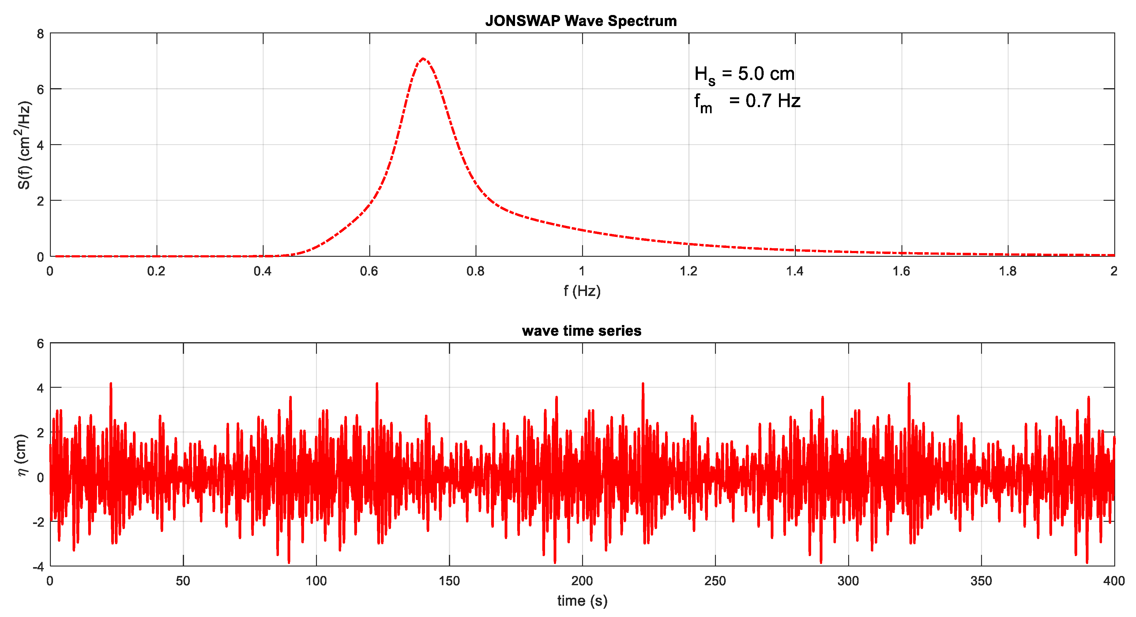
In order to simulate the coupled heave-pitch motions in irregular waves, the JONSWAP (Joint North Sea Wave Project) wave spectrum is used to generate the irregular waves. It is defined by [
30]
where
is the wave frequency,
is the significant wave height,
is the peak frequency,
is the peak enhancement factor, and
is the shape parameter. The values of the parameters listed in
Table 1 are chosen for simulation of the irregular waves [
30]. The wave frequency range is between 0.01 Hz and 2 Hz, and the sampling interval is 0.01 Hz. There are 200 frequency components, and the simulated irregular waves are shown in
Figure 2.
The ship model is the R-Class Icebreaker model, and the principal particulars of the model are listed in
Table 2. According to the strip theory, the related coefficients of Equation (9) are obtained and given in
Table 3. More details can be found in Xu [
30].
Under the initial conditions
at
, Equation (9) can be solved by the fourth-order Runge-Kutta algorithm, and the integral step size is set as
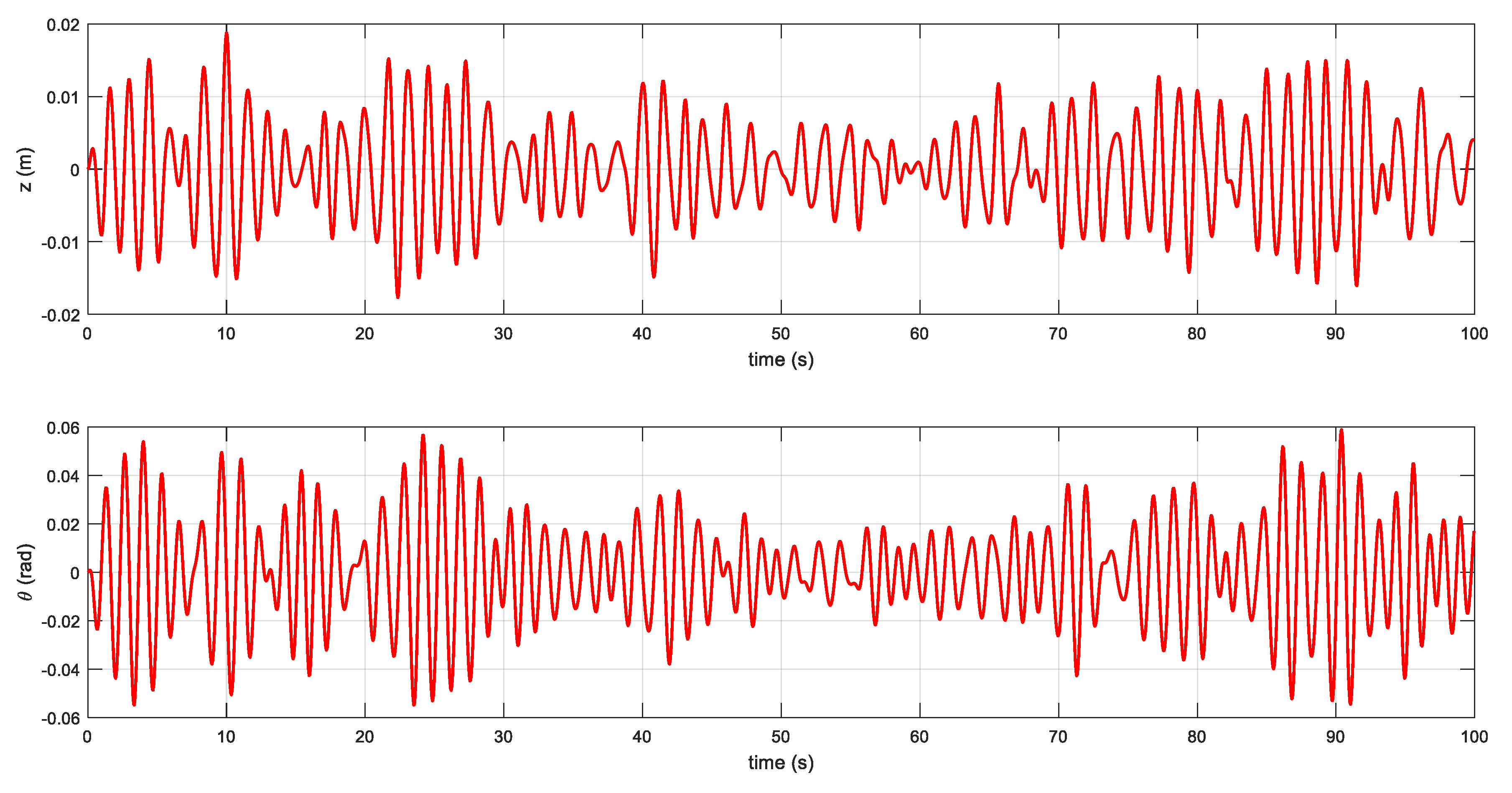
. The simulation results are shown in
Figure 3. There are 1000 samples
, and the sampling interval is 0.1 s. The first three-fifths of the data are used for training, and the rest is used for testing the fixed-grid wavelet network. Before training the wavelet network, the data of coupled heave-pitch motions must be normalized into
. The original output of the system can be obtained by denormalizing the prediction results.
Equation (9) is discretized, and it gives:
where
k denotes the
k-th sampling instant.
It is easy to know that the six input variables in Equation (11) may be the most important. According to the prediction results,
are the most significant terms, and the nonlinear autoregressive (NAR) model is enough to describe the essential characteristics of the coupled heave-pitch motions in irregular waves. The structure of the fixed-grid wavelet networks is set as follows:
where
The functional components
and
in Equation (12) can be fitted by the one- and two-dimensional Mexican-hat radial wavelets. The maximum number of the continuous fine-tuning is not larger than 5. The coarsest resolutions
and the finest resolutions
are set to 0 and 3 in the one-dimensional radial wavelets, and the coarsest resolutions
and the finest resolutions
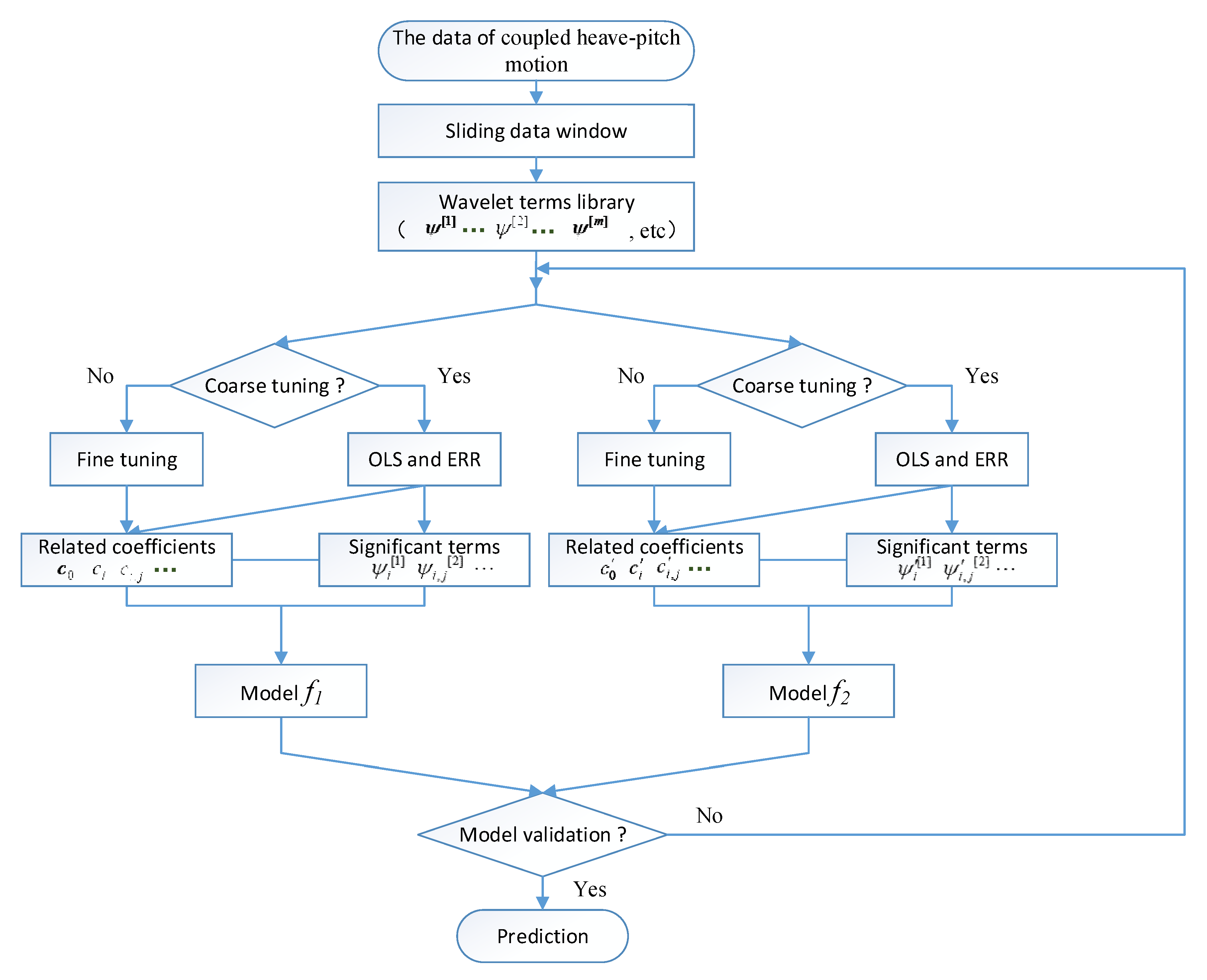
are set to 0 and 2 in the two-dimensional radial wavelets. The sliding data window contains the data of coupled heave-pitch motions for training the wavelet model. The coarse training condition for the wavelet model of heave motion is that the other significant terms must be added in the model when
or
, while the coarse training condition for the wavelet model of pitch motion is
or
, where
represents the root mean square error (
RMSE) of the training data. These values are determined by the trial-and-error approach, and the
RMSE is defined as
where
N represents the number of samples;
is the sample data, and
is the estimated data by the model.
The identified model is given as
where the related coefficients are given in
Table 4. The outputs of the identified model are inversely normalized to obtain the original system outputs.
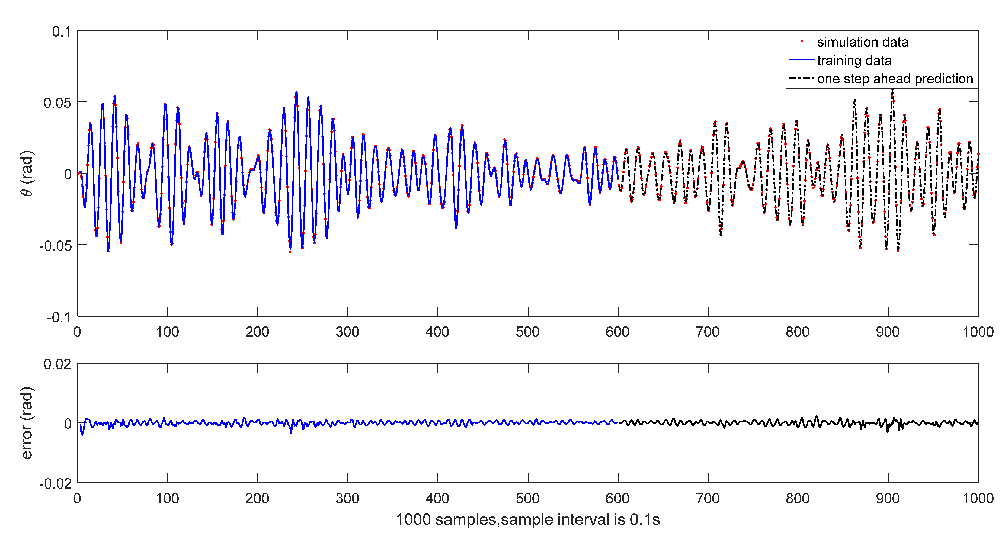
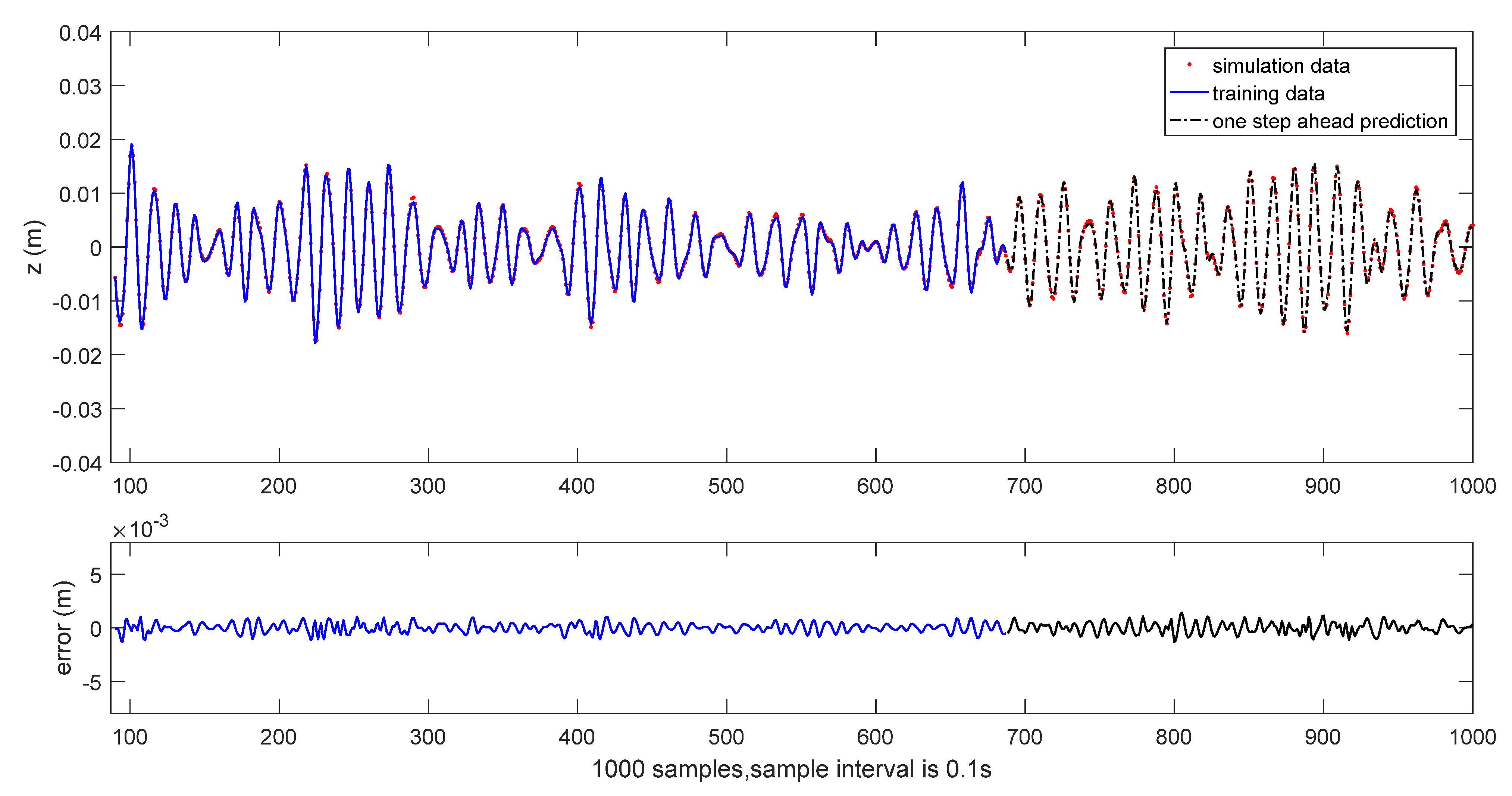
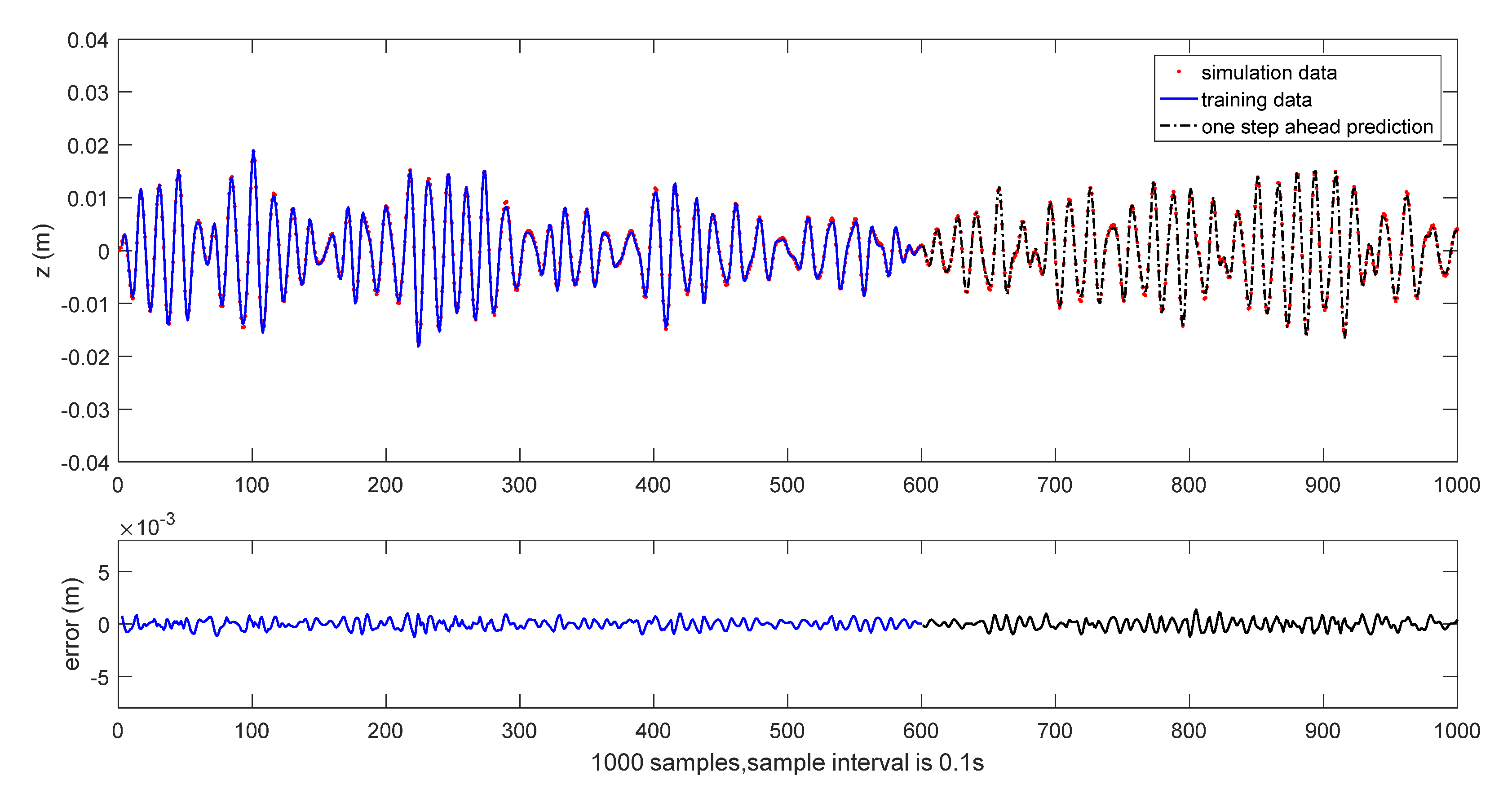
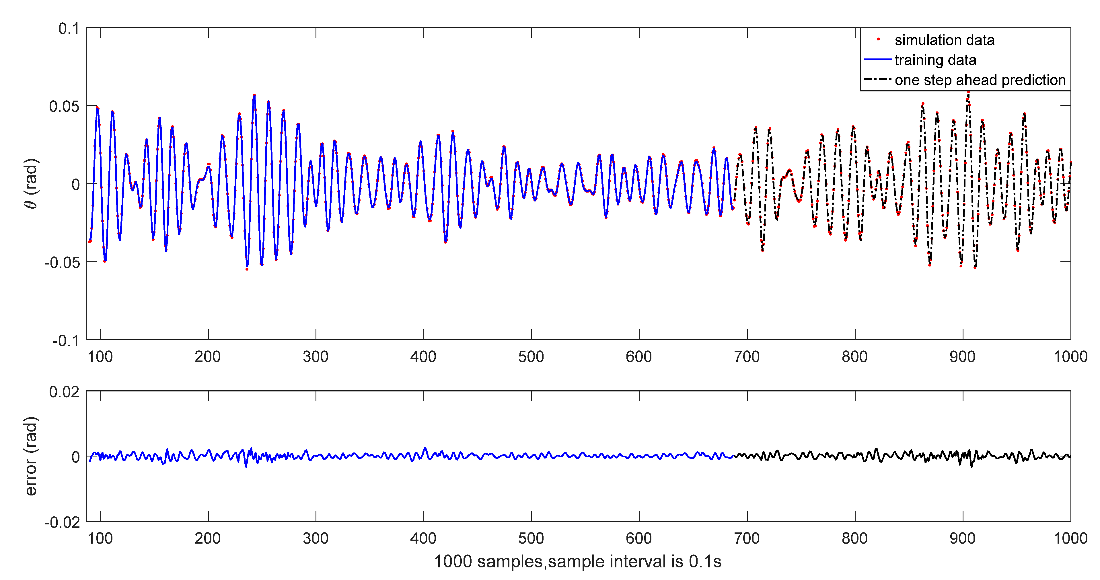
The results of initial one-step ahead prediction are depicted in
Figure 4 and
Figure 5, where the solid line shows the training part, and the dash line shows the testing part. The RMSE of the identified wavelet model is given in
Table 5.
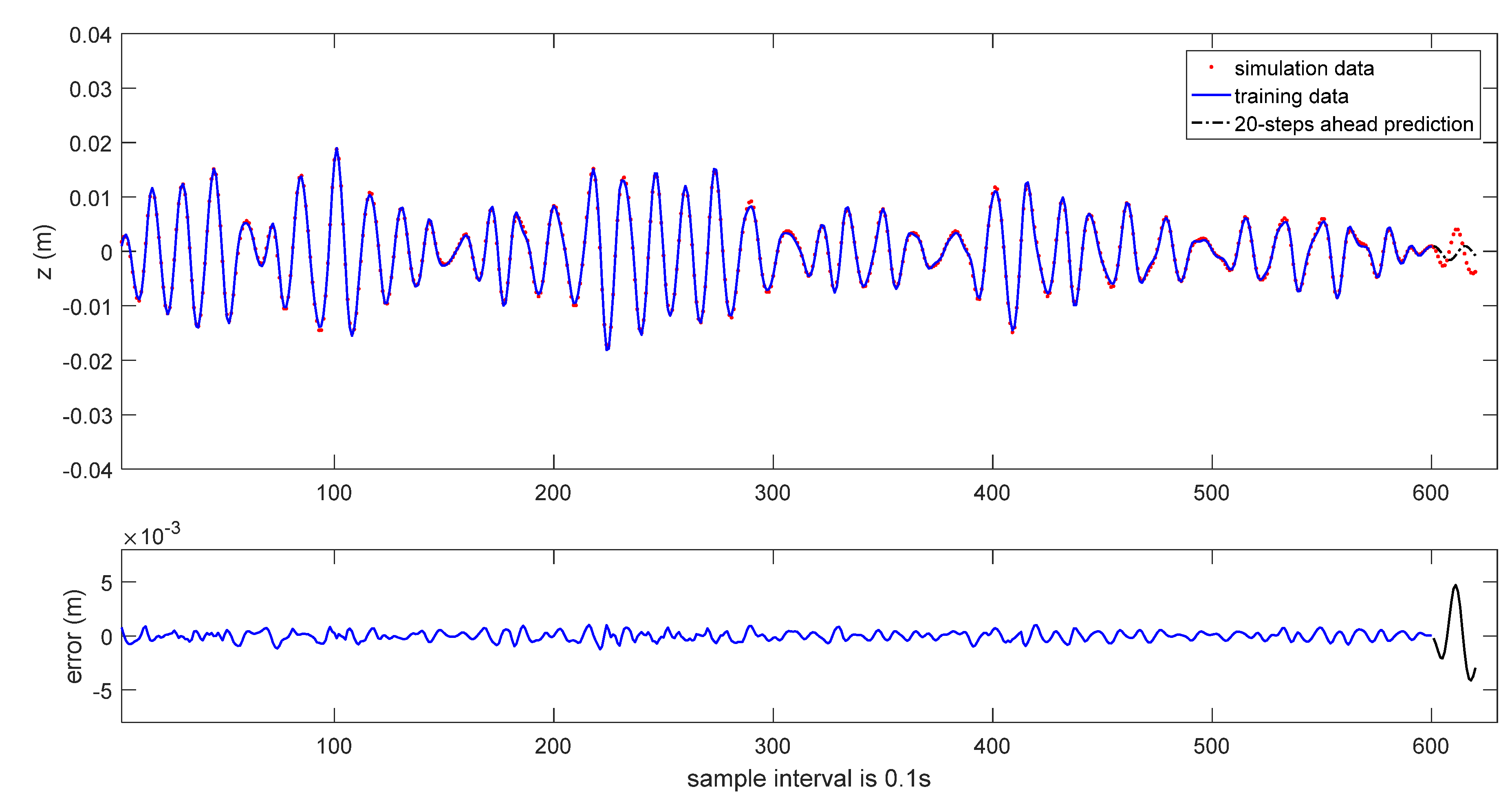
The multi-steps-ahead prediction can be expressed as
where
s represents the prediction instant.
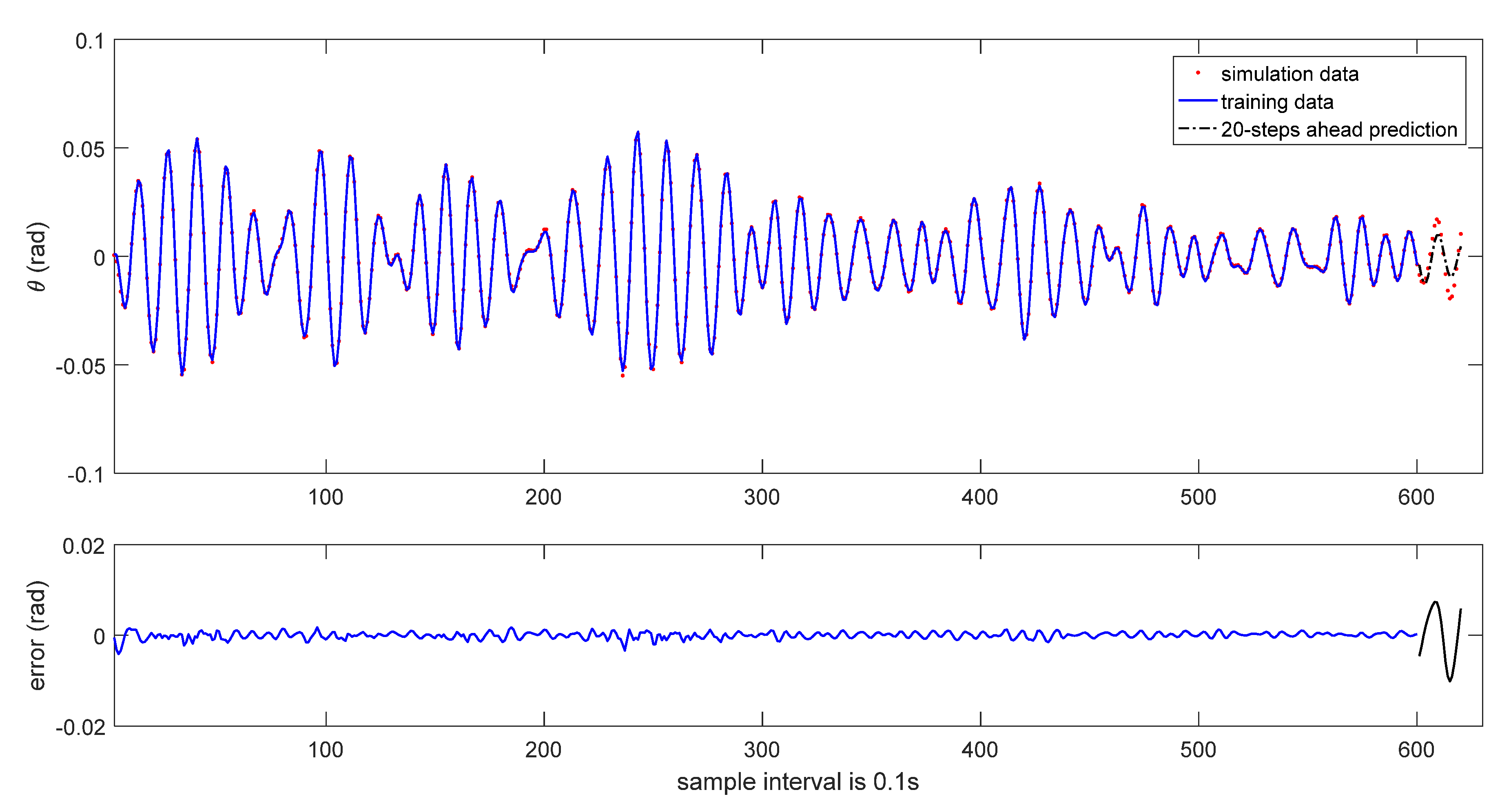
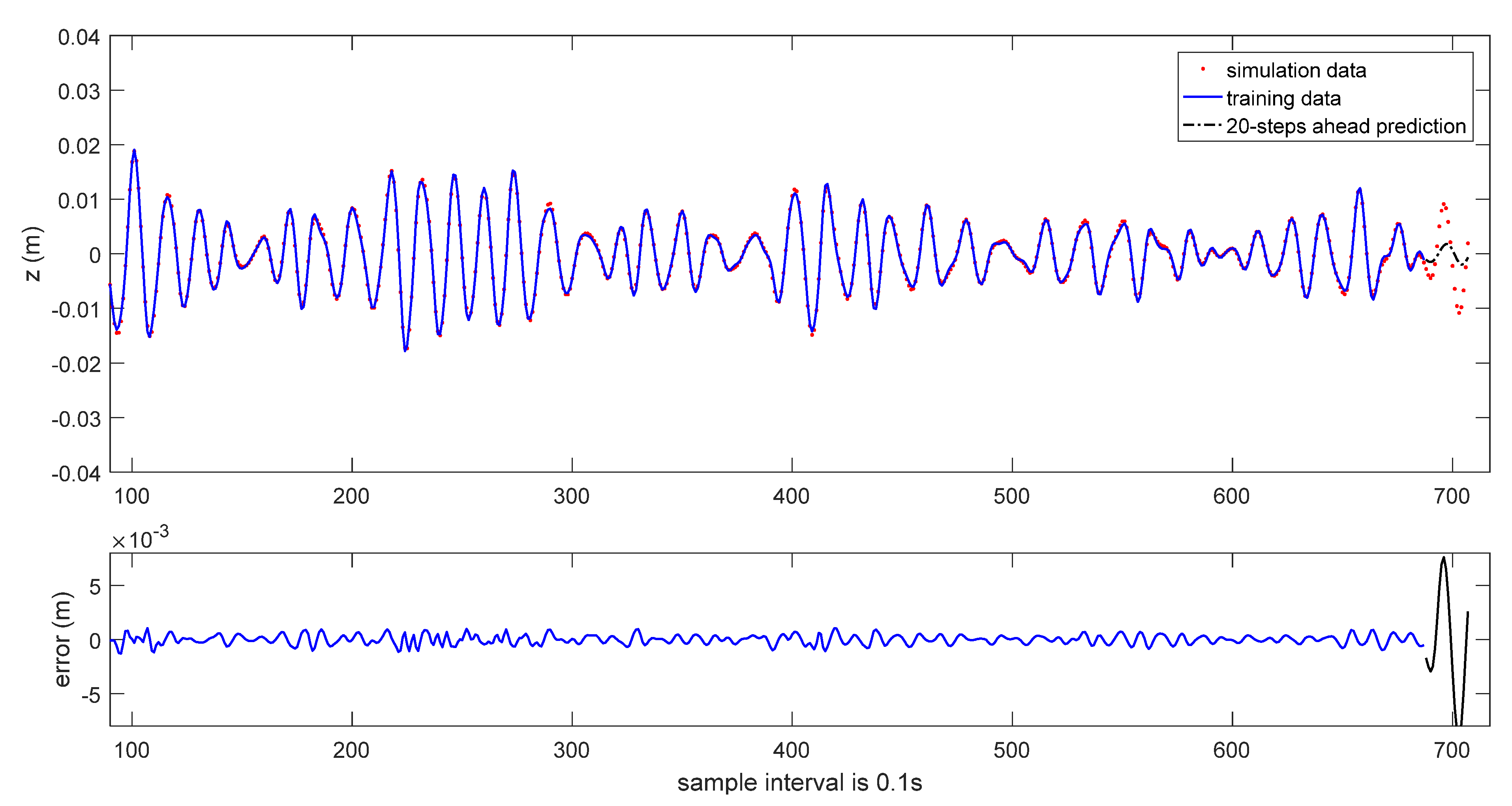
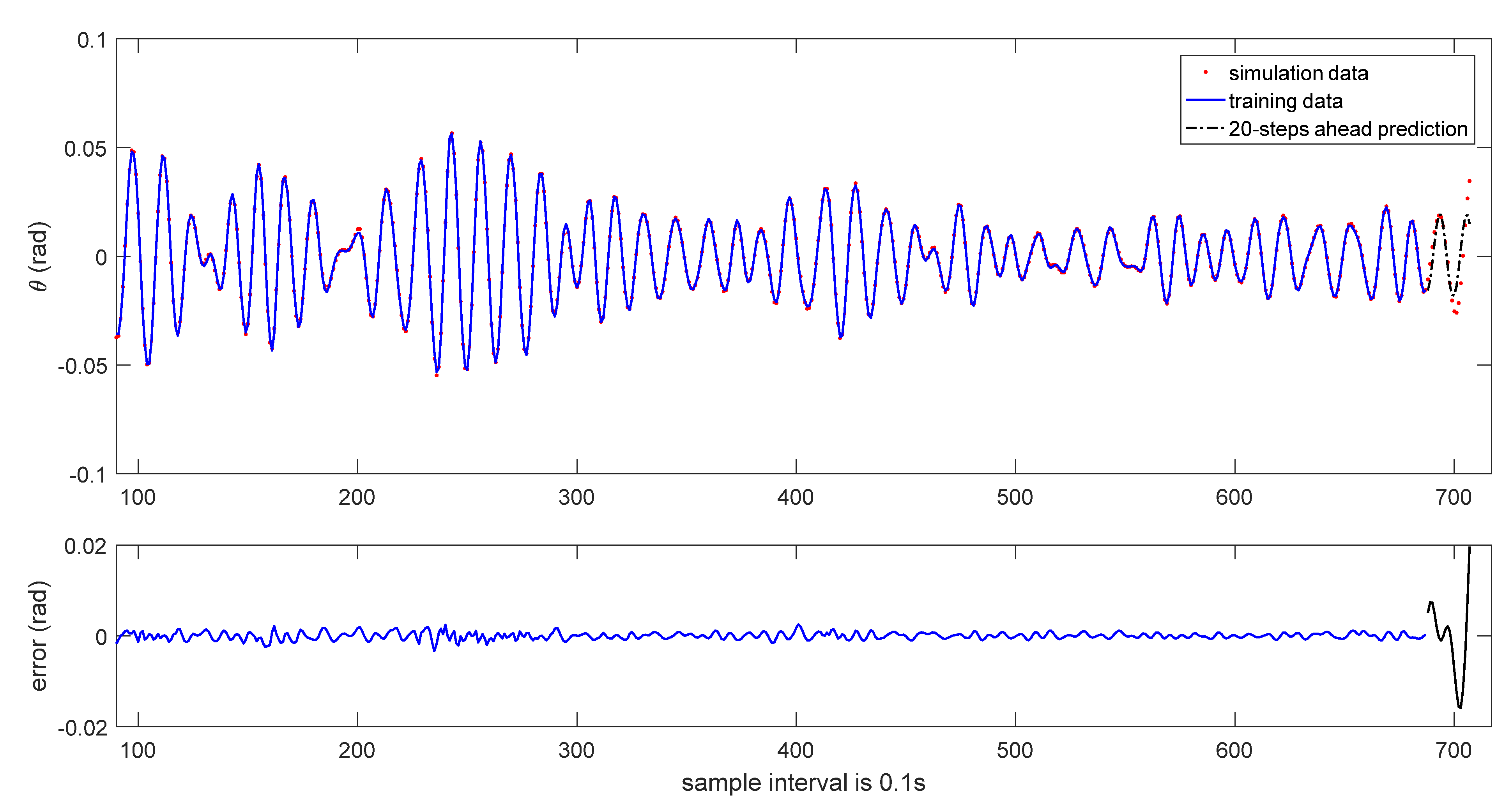
The 20-steps-ahead prediction results are depicted in
Figure 6 and
Figure 7. As it can be seen in these figures, the prediction performance is acceptable. Due to the accumulation of data error, the prediction performance is degraded.
When the sliding data window receives new sample data, the above modeling process will be repeated. For example, as the sliding data window moves to the sampling instant
k = 687, the corresponding identified model is given as follows:
where the related coefficients are listed in
Table 6.
The proposed method is an online modeling method. The structure and parameters of the CFT-FGWN can change online as the sliding data window moves. When the sliding data window receives new sample data, the wavelet model can be adjusted online over time. The dynamic feature of the modeling process is shown in
Figure 12. It shows that several significant wavelet terms can characterize the coupled heave-pitch motions in irregular waves very well. It is also shown clearly that the number of significant wavelet terms changes after the coarse-tuning process, and it is different for heave motion and pitch motion. The number of the continuous fine-tuning does not exceed 5, and the continuous fine-tuning can also satisfy related modeling conditions, which shows that this modeling method is effective.
The computational time of the related modeling algorithm is shown in
Table 7. Obviously, the coarse-tuning process needs more computational time than the fine-tuning process. Hence, the computational efficiency is improved by adding the continuous fine-tuning process.
It is clearly shown that the CFT-FGWN has the ability to represent the coupled heave-pitch motions in irregular waves. As a NAR modeling method, it is not necessary to measure the information of waves. This is an especially beneficial advantage, since the state of the waves is usually difficult to measure online at the open sea. As long as the past state of the coupled heave-pitch motions is obtained, the forecast model can be established online. Besides, it is easy to see that different system inputs contribute differently to the system output; thus, the influences of different system inputs can be distinguished. This is another advantage of the proposed modeling method over the conventional neural network.
4.2. Prediction Results Based on Experimental Data
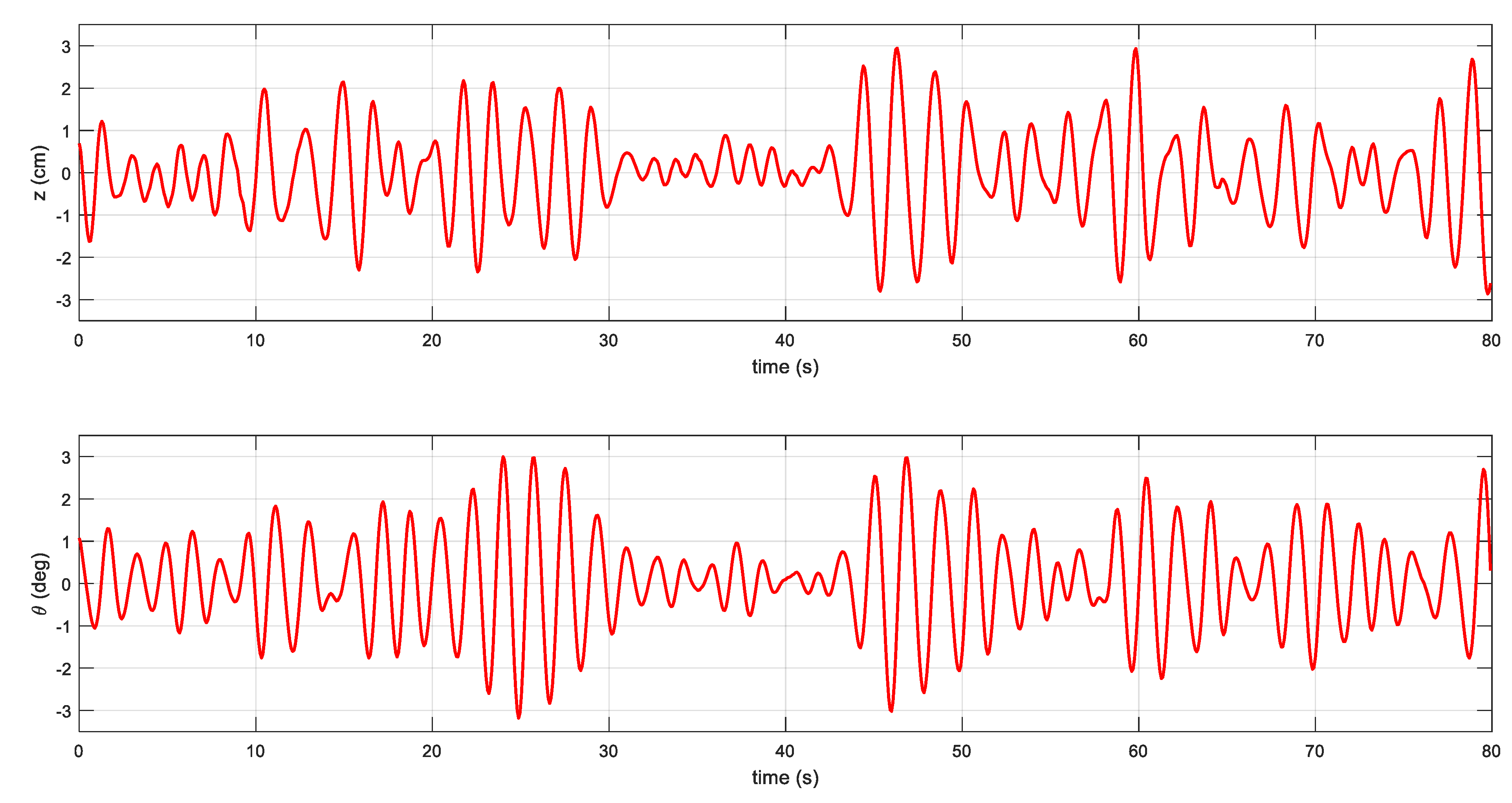
The experimental data of coupled heave-pitch motions of an FPSO model is also used to verify the effectiveness of the proposed modeling method. The experimental data are obtained from the State Key Laboratory of Ocean Engineering at Shanghai Jiao Tong University, and the principal particulars of the FPSO model are given in
Table 8 [
31]. The JONSWAP wave spectrum is used to actuate the FPSO model. The significant wave height and the peak spectral period are 0.1852 m and 1.68 s, respectively. There are 1000 samples, and the sampling interval is 0.08 s, as shown in
Figure 13. The first three-fifths of the data are used for training, and the rest is used for testing. The coarsest resolutions
and the finest resolutions
are set to 0 and 3 in the one-dimensional radial wavelets, and the coarsest resolutions
and the finest resolutions
are set to 0 and 2 in the two-dimensional radial wavelets. The maximum number of the continuous fine-tuning is not larger than 5. The coarse training condition for the wavelet model of heave motion is that the other significant terms must be added in the model when
or
, while the coarse training condition for the wavelet model of pitch motion is
or
. These values are determined by the trial-and-error approach.
The identified model is as follows:
where the related coefficients are given in
Table 9. The outputs of the identified model are inversely normalized to obtain the original system outputs.
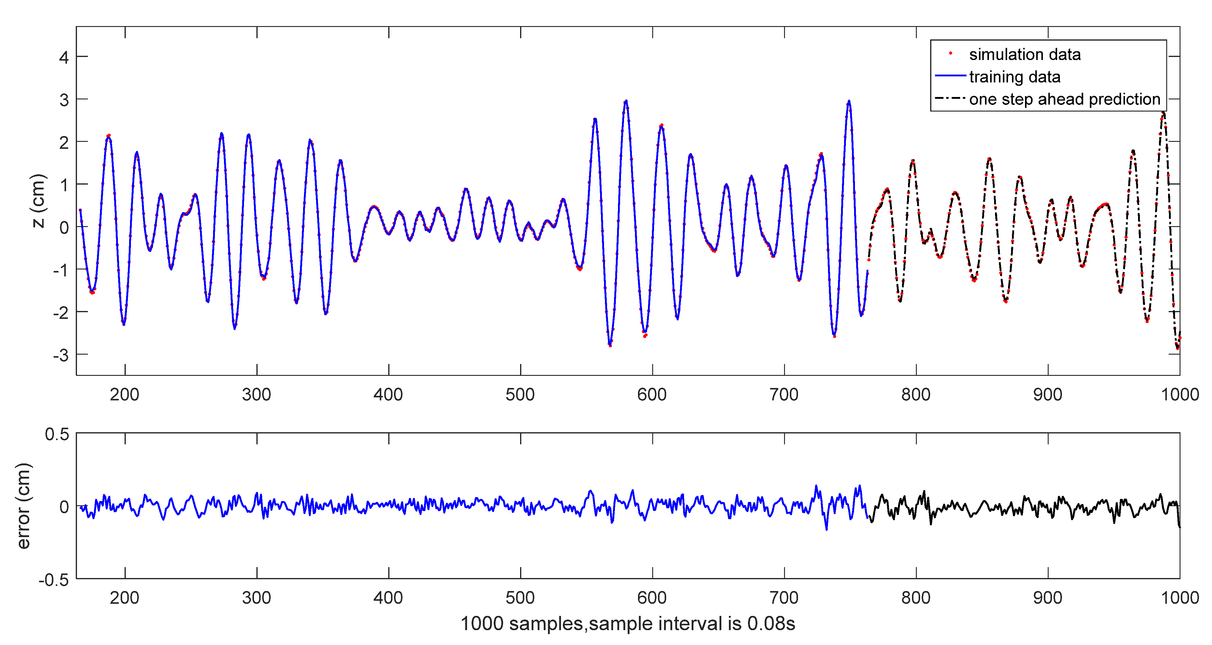
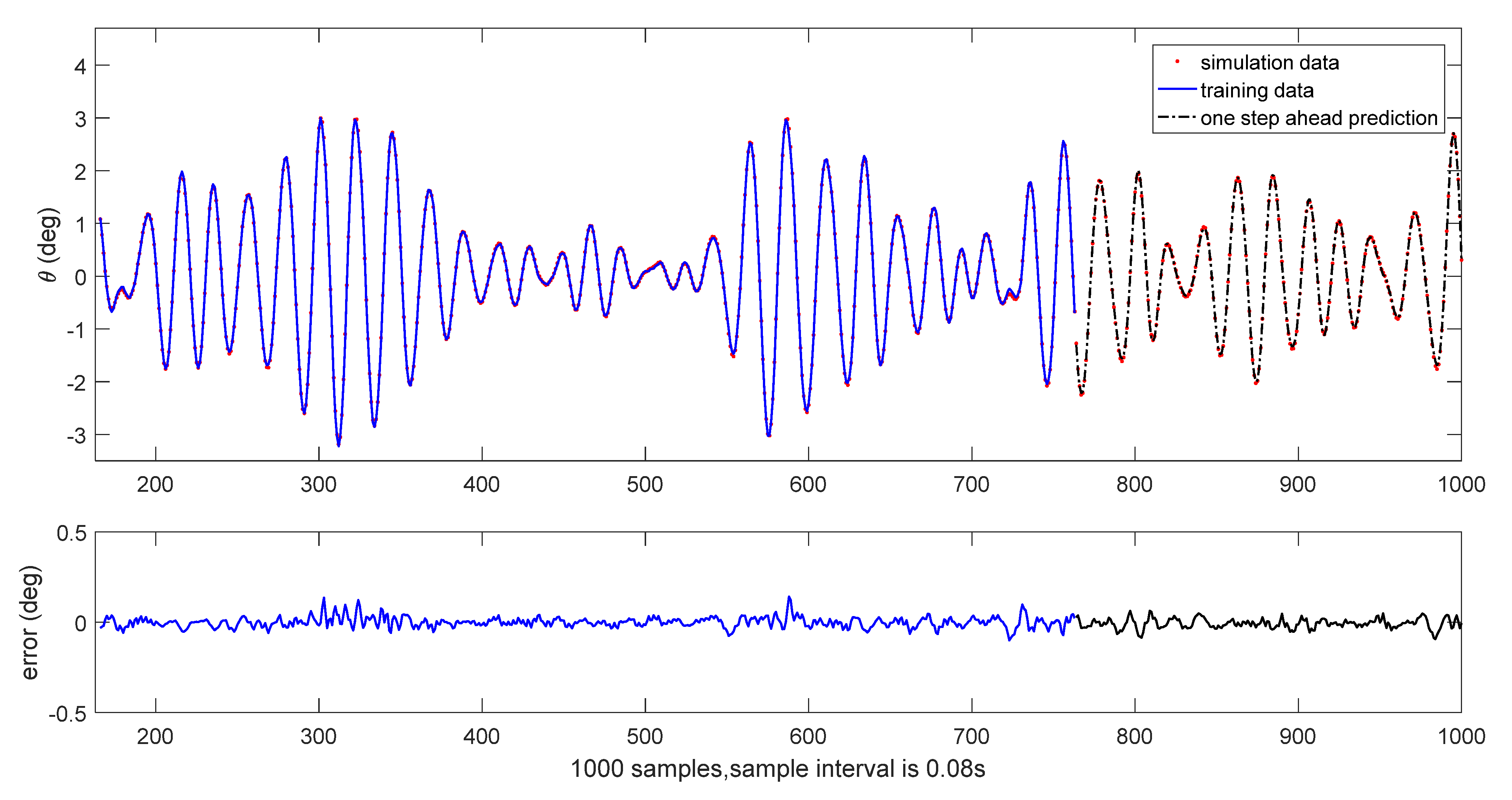
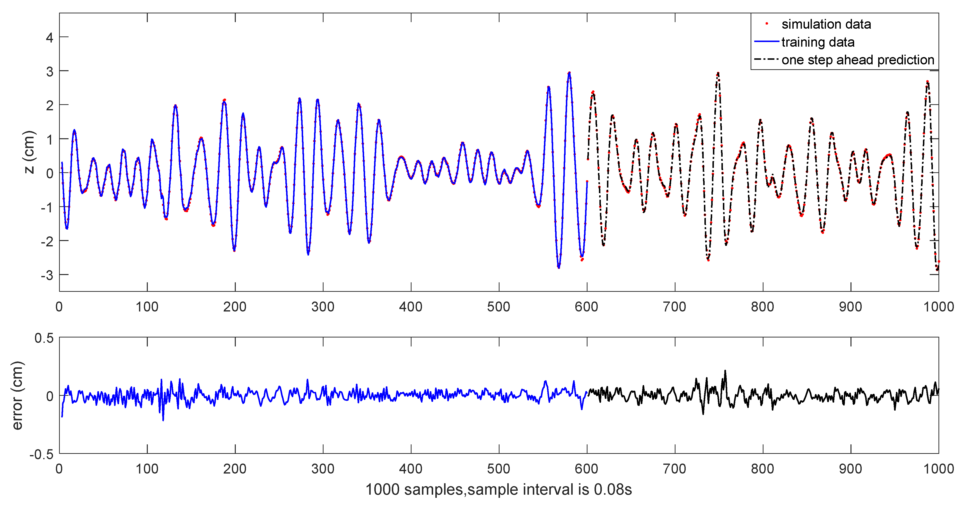
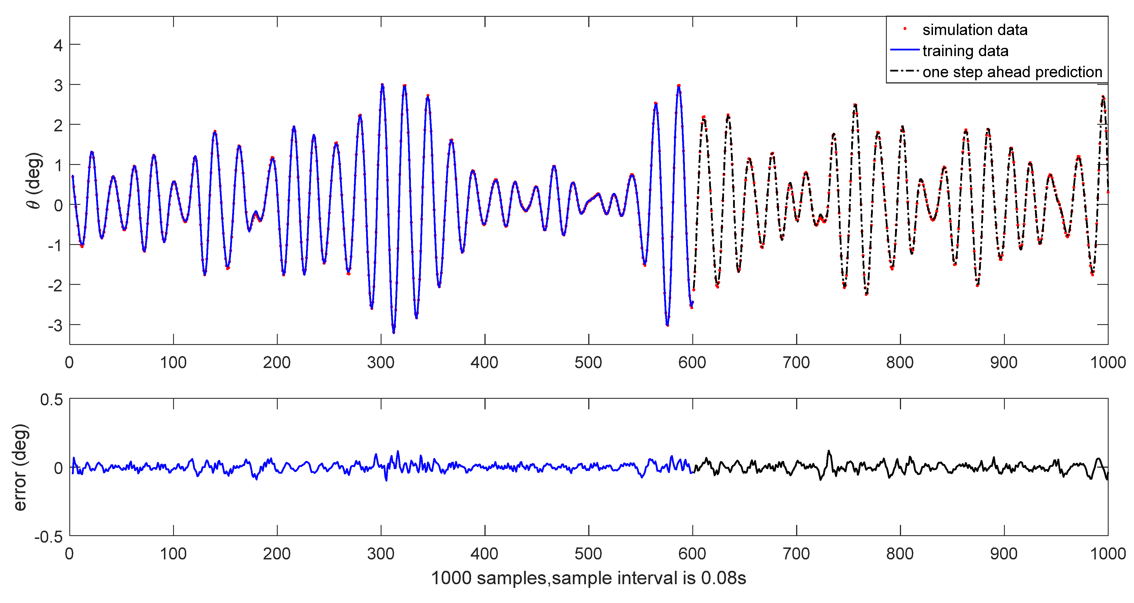
The results of initial one-step ahead prediction are depicted in
Figure 14 and
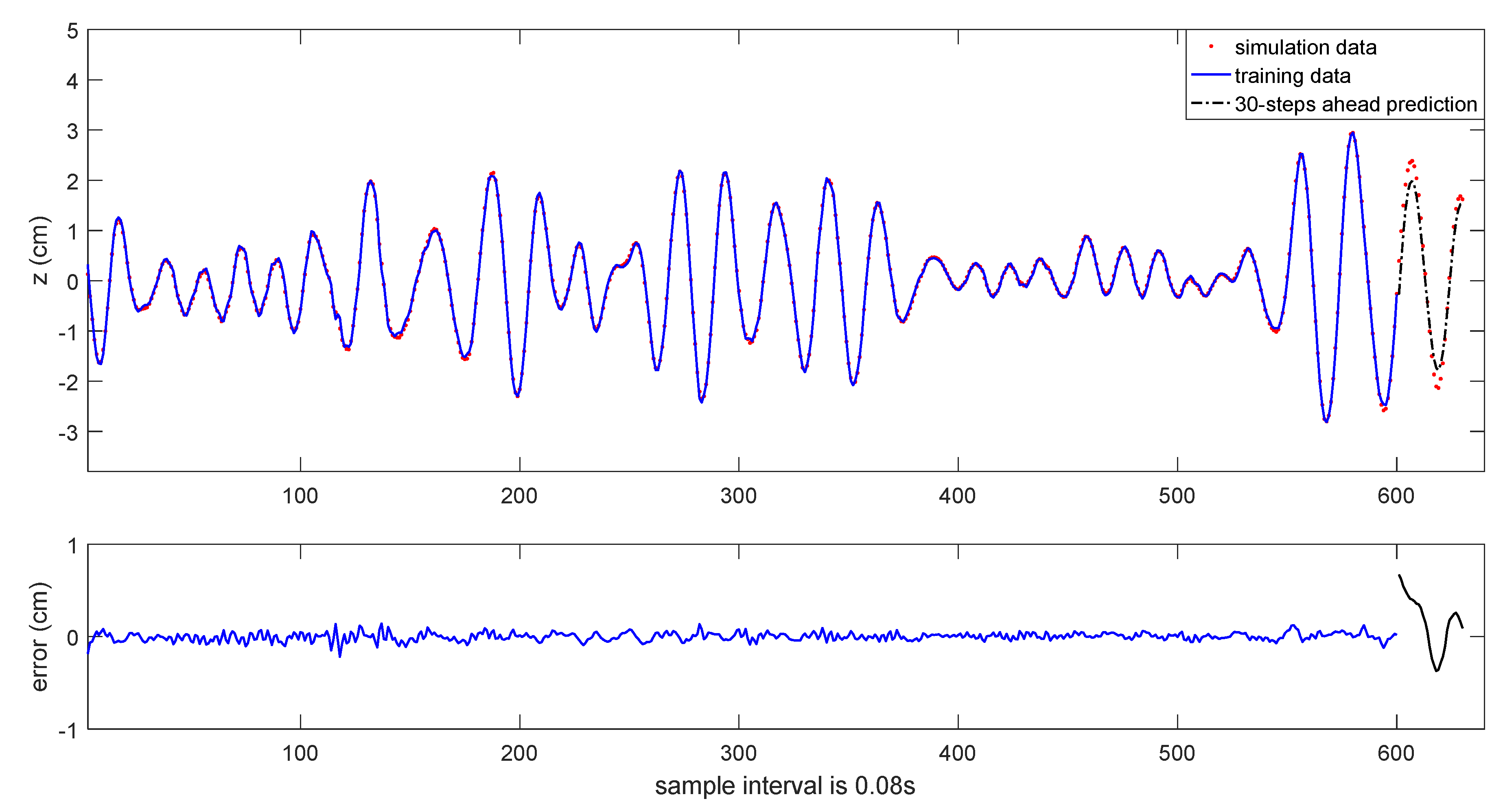
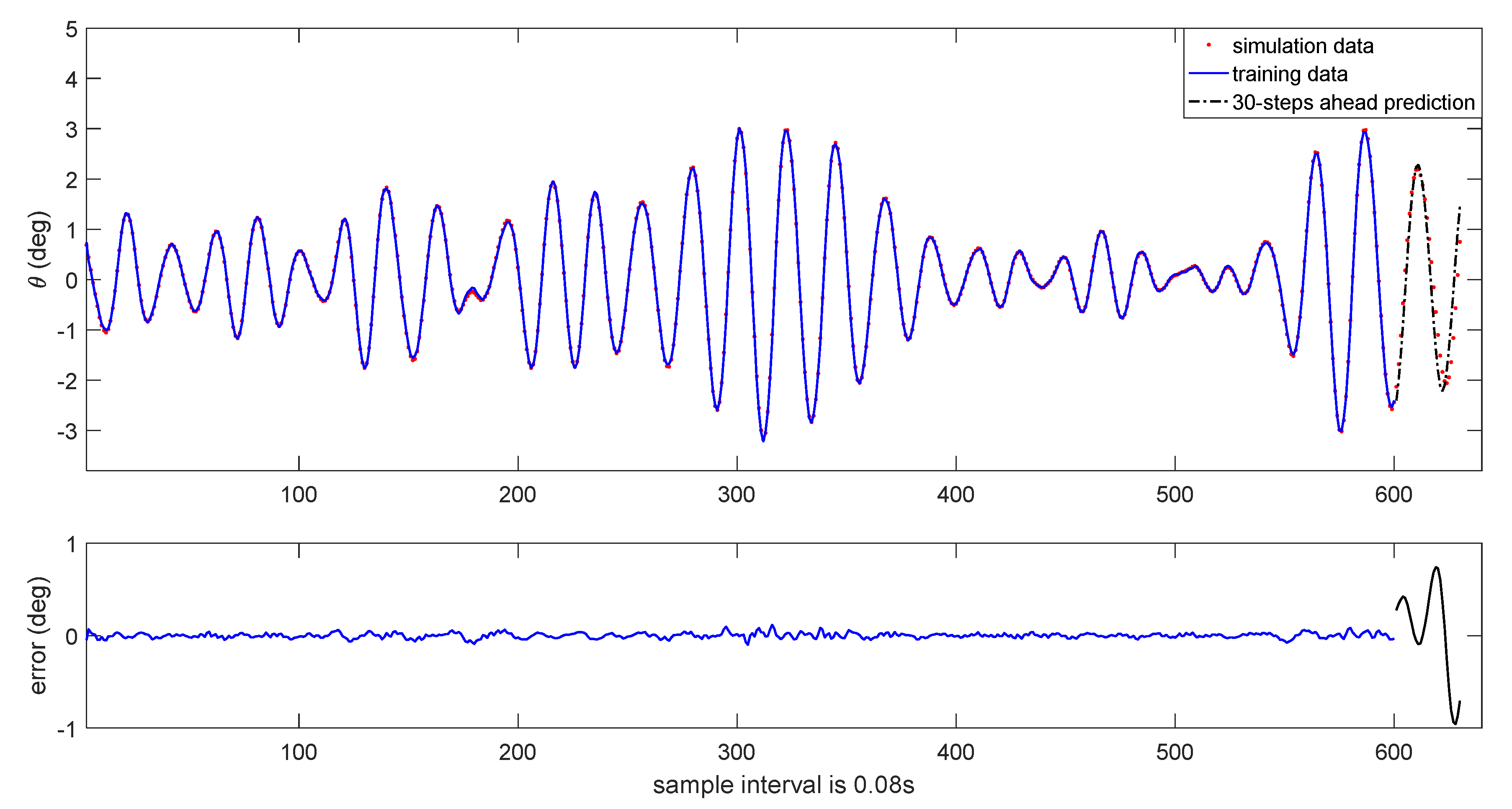
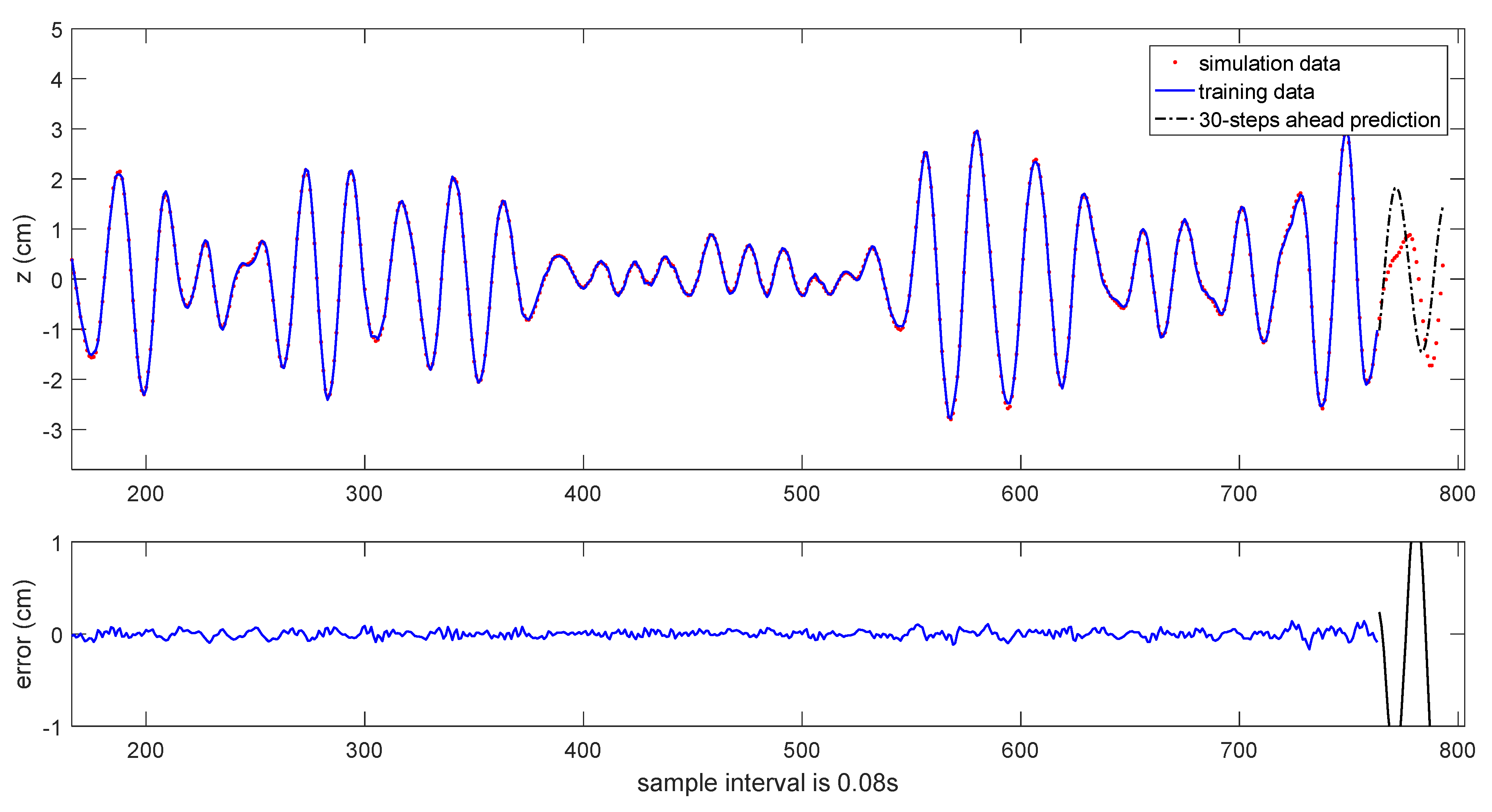
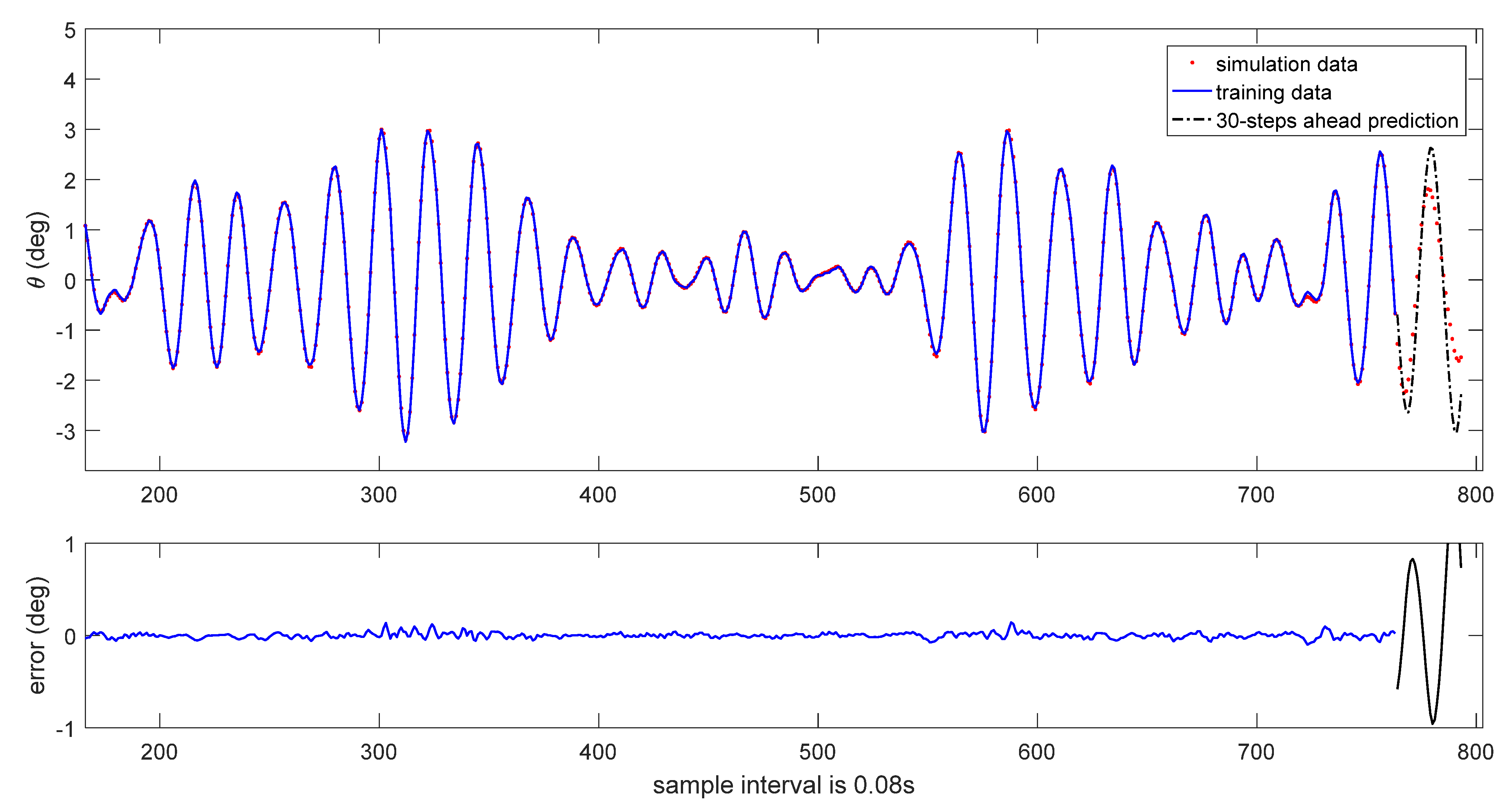
Figure 15. The results of 30-steps-ahead prediction are depicted in
Figure 16 and
Figure 17. It can be seen that the prediction performance is satisfactory.
As the sliding data window continues to move, it receives new data and the model can be adjusted online. For example, when the sliding data window receives the data at the sampling instant
k = 763, the corresponding model is identified as follows:
where the related coefficients are given in
Table 10.
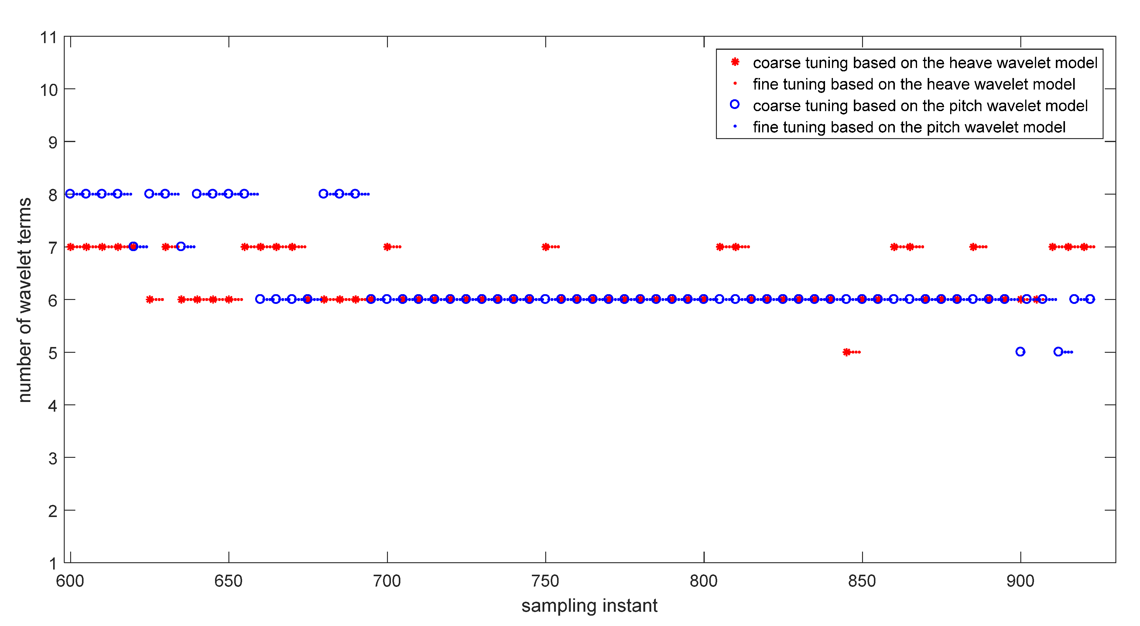
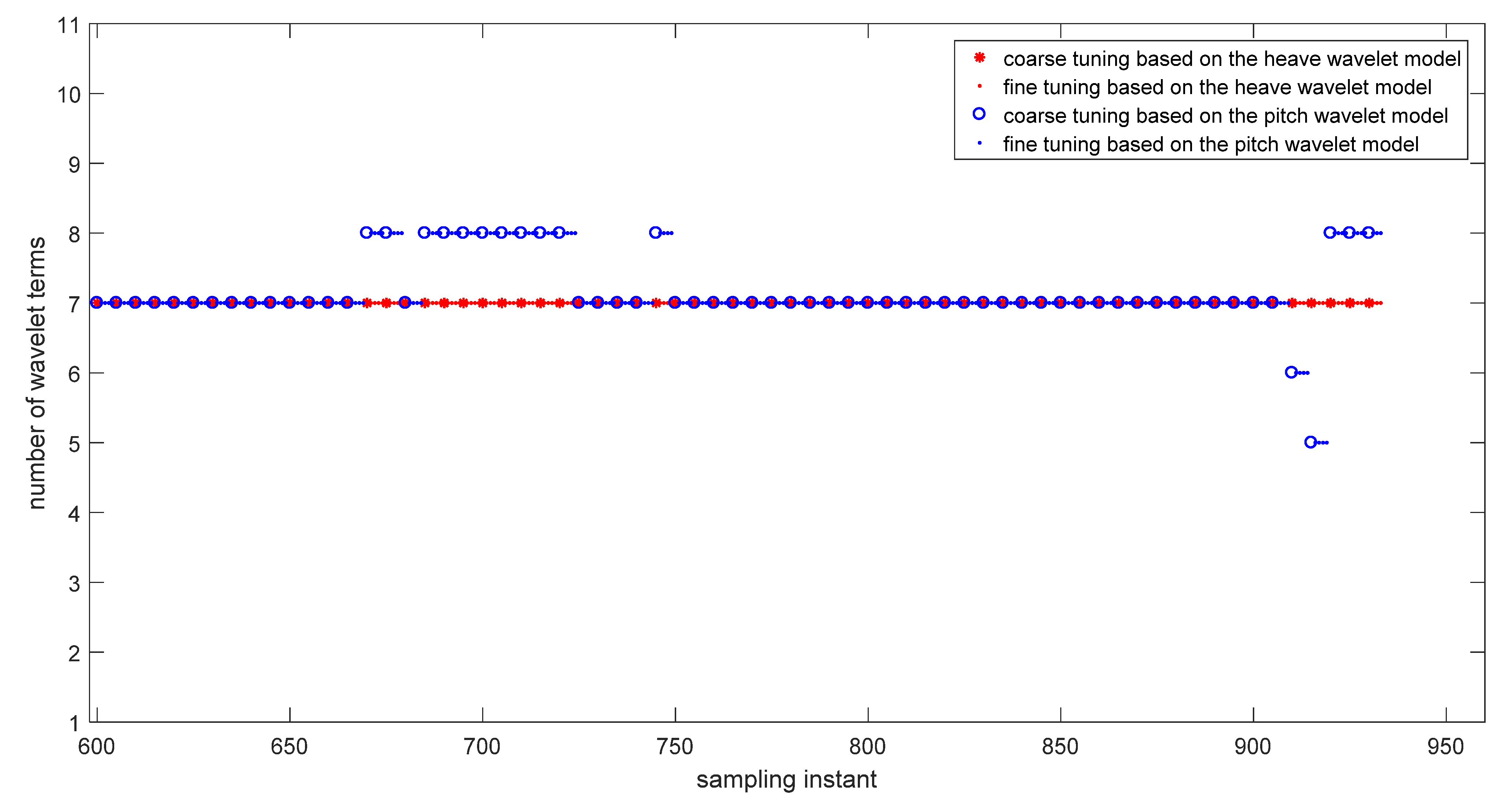
The structure of the CFT-FGWN can be adjusted online over time, and the change process is shown in
Figure 22. It can be seen clearly that several significant wavelet terms can characterize the coupled heave-pitch motions in irregular waves, which shows that the CFT-FGWN has a strong nonlinear fitting ability.
The computational time of the related modeling algorithm is given in
Table 11. It can be seen that the fine-tuning process takes less computational time than the coarse-tuning process. The computational efficiency is improved significantly due to the continuous fine-tuning process.


