Online Prediction of Ship Coupled Heave-Pitch Motions in Irregular Waves Based on a Coarse-and-Fine Tuning Fixed-Grid Wavelet Network

Abstract

A method based on a coarse- and fine-tuning fixed-grid wavelet networks is presented for online prediction of the coupled heave-pitch motions of a ship in irregular waves. The online modeling method contains two processes, i.e., coarse tuning and fine tuning. The coarse tuning is used to select the important wavelet terms, while the fine tuning is only used to compute the related coefficients of the selected wavelet terms. The Givens transformation algorithm is applied to realize the fine-tuning process. Due to the continuous fine-tuning process, the computational efficiency is improved significantly. Both simulation data and experimental data are used to verify the modeling method. The prediction results illustrate that the method has the ability to online predict the coupled heave-pitch motions of a ship in irregular waves.

1. Introduction

Due to the environmental disturbances such as wind, waves and current, it is very difficult to establish a precise mathematical model for ship motion at sea [1]. Over many years, a variety of methods have been proposed and used to predict ship motion. The classic method is Kalman filtering technique; but to use it, the state equation of ship motion must be known first [2,3]. Another commonly used method is time-series-analysis techniques, such as autoregression (AR) model and autoregressive moving average (ARMA) model, which are linear analysis methods. In many cases, they are not suitable for modeling nonlinear ship motion. The computational fluid dynamics (CFD) method is another important method for modeling and predicting ship motion at sea, but ship geometry and environmental information are prerequisites for using it, and it is extremely time consuming.

In recent years, with the development of artificial intelligence (AI) technology, the related machine-learning technology has been widely used in the naval architecture and shipping industry. Back-propagation neural networks have been used to predict ship motion [4,5]. The radial-basis-function neural network was proposed to predict vessels’ heave motion [6], a support vector machine was proposed to predict ship motion [7,8,9], and the adaptive wavelet network was used to predict short term ship motion [10,11]. With the development of deep learning, it has also been applied in ship-motion prediction; a hybrid deep-learning and ARIMA model was used for ships’ roll motion prediction [12]. Recurrent neural network (RNN) is used for predicting the vertical acceleration of a large-scale ship [13]. Convolutional neural networks (CNN) and long short-term memory (LSTM) neural networks are also used for ship-motion prediction. The dual-pass LSTM network is used for ship-heave prediction by Hu et al. [14]. CNN with LSTM is used for roll-motion prediction of unmanned surface vehicles (USVs) by Zhang et al. [15]. Deep-neural-network models usually contain many training parameters; thus, they often need a large number of training samples. Neural networks can theoretically fit arbitrary nonlinear functions with arbitrary precision [16]; because of this advantage, they are also used in ship motion modeling and parameter identification. Haddara and Xu used the random-decrement technique and neural networks to identity the parameters of coupled heave-pitch motion equations [17]. Yin et al. used neural networks to predict ship’s roll motion during maneuvering [18]. Hou et al. used support vector machines to identify the parameters of coupled heave-pitch motions of a ship in regular waves [19]. However, many neural networks trained by gradient-type algorithms are liable to fall into local optimum, and the number of neurons in the hidden layers is not easy to predetermine, especially for online modeling, as the structure of neural networks is difficult to change online.

Among the six degrees of freedom ship motions, the coupled heave-pitch motions are most important for ships’ seakeeping performance, since they are directly related to green water on deck, slamming, propeller racing, etc. Besides, the prediction of coupled heave-pitch motion is very important for motion compensation in marine operations, such as the landing of air vehicles on ship-based platforms, the launching of shipboard weapons, and lifting operations at sea; it is also important for ships’ motion control, especially by using model-predictive control algorithms. Therefore, the prediction of coupled heave-pitch motions of ships in waves has attracted great attention from the ship hydrodynamics community, and many studies have been carried out in this field. However, there are still some challenging issues, such as the online prediction of coupled heave-pitch motions of a ship in waves, which is worth studying.

In this paper, a coarse-and-fine tuning fixed-grid wavelet network (CFT-FGWN) is used to establish the prediction model of coupled heave-pitch motions of a ship in irregular waves, aiming at online prediction of the coupled heave-pitch motions of a ship sailing at sea. The CFT-FGWN was first presented in Huang et al. [20,21] for the online prediction of ships’ roll motion. The modeling method of CFT-FGWN can online change the structure of the wavelet network and avoid local optima, and usually converges fast. This modeling method was used for predicting ships’ roll motion in regular waves [20] and in irregular waves [21]; there was only once fine tuning in these studies. In this paper, continuous fine-tuning is implemented for two degrees of freedom ship motions, i.e., heave and pitch, in irregular waves, which makes the computing efficiency greatly improved. The results show that the online modeling method can effectively predict the coupled heave-pitch motions of a ship in irregular waves.

2. Fixed-Grid Wavelet Networks for a Multiple-Inputs Multiple-Outputs System

In general, a multiple-inputs multiple-outputs (MIMO) system can be represented as

$$\{\begin{array}{l}{y}_1(t)=f_1(x_1(t),x_2(t),\cdots ,x_n(t))+e_1(t)\\ y_2(t)=f_2(x_1(t),x_2(t),\cdots ,x_n(t))+e_2(t)\\ \hspace{1em}\hspace{1em}⋮\\ y_m(t)=f_m(x_1(t),x_2(t),\cdots ,x_n(t))+e_m(t)\end{array}$$

(1)

where $\mathit{x}(t)={[x_1(t),x_2(t),\cdots ,x_n(t)]}^{\mathrm{T}}$ and $\mathit{y}(t)={[y_1(t),y_2(t),\cdots ,y_m(t)]}^{\mathrm{T}}$ are the system input vector and system output vector, respectively; $\mathit{e}(t)={[e_1(t),e_2(t),\cdots ,e_m(t)]}^{\mathrm{T}}$ is the system noise vector; n and m are the numbers of input variables and output variables of the system, respectively. A neural network is a typical MIMO system model. By simple mathematical decomposition, it can also be expressed in the form of Equation (1). In fact, each MIMO system can be thought of as a combination of multiple-inputs single-output (MISO) systems, and each MISO system can be described by a multivariate nonlinear function. In this paper, a combination of wavelet-basis functions is used to represent this nonlinear function.

According to wavelet theory, the multivariate nonlinear function $f(x_1(t),x_2(t),\cdots ,x_n(t))$ can be expressed as [20,21,22,23,24]

$$\begin{array}{r}f(x_1(t),x_2(t),\cdots ,x_n(t))=c_0+{\displaystyle \sum _{i=1}^n}{c}_i{\psi }^{[1]}(x_i(t))+{\displaystyle \sum _{1<i<j\le n}}{c}_{i,j}{\psi }^{[2]}(x_i(t),x_j(t))+\cdots \\ +{\displaystyle \sum _{1<i_1<\cdots <i_m\le n}}{c}_{i,i_2,\cdots ,i_m}{\psi }^{[m]}(x_{i_1}(t),x_{i_2}(t),\cdots x_{i_m}(t))+\cdots +e(t)\hspace{1em}\hspace{1em}i,j\in Z\end{array}$$

(2)

where $c_0$ is a constant component representing the intrinsic varying trend; ${\psi }^{[1]}(\cdot )$, ${\psi }^{[2]}(\cdot )$ and ${\psi }^{[m]}(\cdot )$ are the univariate, bivariate and m-dimensional wavelet-basis functions, respectively; and $c_i$, $c_{i,j}$ and $c_{i_1,i_2,\cdots ,i_m}$ are the coefficients of the corresponding wavelet-basis functions. Equation (2) can be seen as the structure of the fixed grid wavelet network. Due to this variety of wavelet-basis functions, different wavelet-basis functions can be selected for different nonlinear systems. Especially for strongly nonlinear systems, the fixed-grid wavelet network usually converges very quickly.

In order to predict the coupled heave-pitch motions of a ship with two degrees of freedom, the model for this multivariate nonlinear system can be expressed as

$$\{\begin{array}{c}\begin{array}{l}{f}_1(x(t))=c_0+{\displaystyle \sum _{i=1}^n{c}_i{\psi }^{[1]}(x_i(t))}+{\displaystyle \sum _{1<i<j\le n}{c}_{i,j}{\psi }^{[2]}(x_i(t),x_j(t))}+\cdots \\ \hspace{1em}\hspace{1em}\hspace{1em}+{\displaystyle \sum _{1<i_1<\cdots <i_m\le n}{c}_{i_1,i_2,\cdots ,i_m}{\psi }^{[m]}(x_{i_1}(t),x_{i_2}(t),\cdots x_{i_m}(t))}+\cdots +e_1(t)\end{array}\\ \begin{array}{l}{f}_2(x(t))={c^{\prime }}_0+{\displaystyle \sum _{i=1}^n{c^{\prime }}_i{{\psi }^{\prime }}^{[1]}(x_i(t)})+{\displaystyle \sum _{1<i<j\le n}{c^{\prime }}_{i,j}{{\psi }^{\prime }}^{[2]}(x_i(t),x_j(t))}+\cdots \\ \hspace{1em}\hspace{1em}\hspace{1em}+{\displaystyle \sum _{1<i_1<\cdots <i_m\le n}{c^{\prime }}_{i_1,i_2,\cdots ,i_m}{{\psi }^{\prime }}^{[m]}(x_{i_1}(t),x_{i_2}(t),\cdots x_{i_m}(t))}+\cdots +e_2(t)\end{array}\end{array}$$

(3)

where $f_1(\cdot )$ and $f_2(\cdot )$ are the nonlinear functions of heave motion and pitch motion, respectively. Thus, the key problem of the modeling method is how to determine these wavelet terms and their corresponding coefficients. The coarse tuning has the ability to select more important univariate wavelet-basis functions, bivariate wavelet-basis functions and other wavelet-basis functions, while the fine tuning is used to determine the coefficients of the corresponding terms.

3. Coarse-Tuning and Fine-Tuning Algorithm

The coarse-tuning process can choose different important terms in the wavelet library, while the fine tuning only computes the coefficients of the selected important terms. The flow chart of the coarse-tuning and fine-tuning algorithm for the coupled heave-pitch motion modeling is shown in Figure 1. The dataset of coupled heave-pitch motions is a time series. Before modeling, this dataset must be normalized. The sliding data window is a data sequence; the sampling data entering the queue first go out first. The data in the sliding data window are used to establish the prediction model of the coupled heave-pitch motions. The wavelet library contains many different types of wavelet-basis functions; the variety is rich; the representation ability is strong. The orthogonal least squares (OLS) algorithm and error reduction ratio (ERR) criterion can quickly find the more important wavelet-basis functions in the library. First the most important, then the second most important, one after the other until the model meets the accuracy requirement of the design. After finding out the important wavelet-basis functions, the model is fine-tuned by the Givens transformation algorithm, that is, the corresponding coefficients of the selected wavelet-basis functions are calculated. The combination of coarse tuning and fine tuning can determine the corresponding nonlinear model effectively. With the sliding data window moving, the prediction model of coupled heave-pitch motions can be established online.

The OLS algorithm and ERR criterion are applied to realize the coarse-tuning process. The ${\mathrm{ERR}}_i$ caused by $q_i(t)$ is defined as [20,21,25,26]

$${\mathrm{ERR}}_i=\frac{{\langle Y(t),q_i(t)\rangle }^2}{\langle Y(t),Y(t)\rangle \langle q_i(t),q_i(t)\rangle }\times 100\%,\hspace{1em}\begin{array}{cc}& i=1,2,\cdots ,\end{array}$$

(4)

where $Y(t)$ is the output vector; $q_i(t)$ is the orthogonal column of the corresponding wavelet terms. The greater the ${\mathrm{ERR}}_i$, the more important the corresponding wavelet term. According to the ${\mathrm{ERR}}_i$ and model validation conditions, the structure of the fixed-grid wavelet networks can be easily determined.

The Givens transformation algorithm is applied to realize the fine-tuning process. The task of fine tuning is to online compute the coefficients of the selected wavelet terms, and the recursive transformation can be expressed as follows [20,21]:

$$\begin{array}{ccc}\left[\begin{array}{cc}{R}_{m(t)\times m(t)}(t)& V_{m(t)\times 1}(t)\\ {\psi }_1(t+1),\cdots ,{\psi }_{m(t)}(t+1)& y(t+1)\end{array}\right]& \stackrel{\begin{array}{cc}\mathrm{Givens}& \mathrm{rotation}\end{array}}{\to }& \left[\begin{array}{cc}{R}_{m(t)\times m(t)}(t+1)& V_{m(t)\times 1}(t+1)\\ O_1& \xi (t+1)\end{array}\right]\\ & & \downarrow \\ & & \left[\begin{array}{cc}{R}_{m(t)\times m(t)}(t+1)& V_{m(t)\times 1}(t+1)\\ O_1& O_2\end{array}\right]\end{array}$$

(5)

where m(t) is the number of the significant components at the instant t after the coarse tuning; $R_{m(t)\times m(t)}(t)$ is a unit upper triangular matrix at the instant t; $V_{m(t)\times 1}(t)$ is a column vector at the instant t that depends on the system output; $[{\psi }_1(t+1),\cdots ,{\psi }_{m(t)}(t+1)]$ are the outputs of wavelet terms depending on the system input at the instant t + 1; $y(t+1)$ is the system output at the instant t + 1; $O_1$ and $O_2$ are the corresponding zero matrixes, respectively; $\xi (t+1)$ represents the error at the instant t + 1. The estimation of ${\mathrm{\Theta }}_{m(t)\times m(t)}(t)$ is equal to $R_{m(t)\times m(t)}^{-1}(t)V_{m(t)\times 1}(t)$.

For the sparse matrix on the left-hand side of Equation (5), the Givens transformation algorithm is described as follows:

$$\begin{array}{l}\mathrm{For}i=1:m(t)\\ \hspace{1em}\hspace{1em}r=\sqrt{{\mathrm{A}}^2(i,i)+{\mathrm{A}}^2(m(t)+1,i)};\\ \hspace{1em}\hspace{1em}c=\frac{\mathrm{A}(i,i)}{r},s=\frac{\mathrm{A}(m(t)+1,i)}{r};\\ \hspace{1em}\hspace{1em}\mathrm{For}j=i:m(t)+1\\ \hspace{1em}\hspace{1em}\hspace{1em}\hspace{1em}\mathrm{A}(i,j)=c\mathrm{A}(i,j)+s\mathrm{A}(m(t)+1,j);\\ \hspace{1em}\hspace{1em}\hspace{1em}\hspace{1em}\mathrm{A}(m(t)+1,j)=-s\mathrm{A}(i,j)+c\mathrm{A}(m(t)+1,j);\\ \hspace{1em}\hspace{1em}\mathrm{End}\\ \mathrm{End}\end{array}$$

(6)

where $\mathbf{A}(i,j)$ represents the $i$-th row and $j$-th column element of the sparse matrix. Yet there is a drawback: if the sparse matrix is decomposed continuously by the Givens transformations, the first element of matrix $R(t)$ will tend to infinite, which may cause the ill-condition of matrix $R(t)$. This problem can be overcome by the back-operation, which is a reverse operation to eliminate the impact of the oldest data in the sliding data window [27,28]. The algorithm is as follows:

$$\begin{array}{l}\mathrm{For}i=1:m(t)\\ \hspace{1em}\hspace{1em}r=\mathbf{A}(i,i);\\ \hspace{1em}\hspace{1em}c=\frac{\sqrt{{\mathbf{A}}^2(i,i)+{\mathbf{A}}^2(m(t)+1,i)}}{r},s=\frac{\mathbf{A}(m(t)+1,i)}{r};\\ \hspace{1em}\hspace{1em}\mathrm{For}j=i:m(t)+1\\ \hspace{1em}\hspace{1em}\hspace{1em}\hspace{1em}\mathbf{A}(i,j)=\frac{\mathbf{A}(i,j)-s\mathbf{A}(m(t)+1,j)}{c};\\ \hspace{1em}\hspace{1em}\hspace{1em}\hspace{1em}\mathbf{A}(m(t)+1,j)=c\mathbf{A}(m(t)+1,j)-s\mathbf{A}(i,j);\\ \hspace{1em}\hspace{1em}\mathrm{End}\\ \mathrm{End}\end{array}$$

(7)

By eliminating the impact of the oldest data and adding the impact of the latest data, the parameter vector can be updated in an iterative way. In order to ensure the flexibility of the model’s structure, the maximum number for the continuous fine-tuning should not be set too large.

4. Simulation Results and Discussion

Based on the simulation data and the experimental data of coupled heave-pitch motions in irregular waves, the proposed CFT-FGWN is used to establish the forecast model of coupled heave-pitch motions. All the programs are executed by MATLAB R2016b under the condition of Intel^® Core™ i5-3230 (CPU) and 8.00 GB memory (RAM).

4.1. Prediction Results Based on Simulation Data

The coupled heave-pitch motions of a ship in irregular waves can be represented by two coupled second-order linear ordinary differential equations, which can be written in the following form [29]:

$$\{\begin{array}{c}\left(m_0+m_{33}\right)\ddot{z}+N_{33}\dot{z}+C_{33}z+(m_{35}-m_0{x}_G)\ddot{\theta }+N_{35}\dot{\theta }+C_{35}\theta ={\tau }_3\\ \left(I_{22}+m_{55}\right)\ddot{\theta }+N_{55}\dot{\theta }+C_{55}\theta +(m_{53}-m_0{x}_G)\ddot{z}+N_{53}\dot{z}+C_{53}z={\tau }_5\end{array}$$

(8)

where $z$ and $\theta$ are the heave displacement and pitch angle, respectively; $x_G$ is the longitudinal coordinate of the center of gravity of the ship; $m_0$ is the mass; $I_{22}$ is the pitch moment of inertia; $m_{33}$ and $m_{55}$ are the added mass and added moment of inertia, respectively; $N_{33}$ and $N_{55}$ are the damping coefficients, respectively; $C_{33}$ and $C_{55}$ are the restoring force coefficients, respectively; $m_{ij}$, $N_{ij}$, and $C_{ij}$ (i, j = 3, 5) are the coupled coefficients; ${\tau }_3$ and ${\tau }_5$ are the wave exciting force and moment, respectively.

After the normalization of the second-order derivative terms in Equation (8), the normalized differential equations of coupled heave-pitch motions can be obtained [19]:

$$\{\begin{array}{c}\ddot{z}+b_{33}\dot{z}+b_{35}\dot{\theta }+r_{33}z+r_{35}\theta ={{\tau }^{\prime }}_3\\ \ddot{\theta }+b_{53}\dot{z}+b_{55}\dot{\theta }+r_{53}z+r_{55}\theta ={{\tau }^{\prime }}_5\end{array}$$

(9)

where

$$\begin{gathered} \left(\begin{array}{cc}{b}_{33}& b_{35}\\ b_{53}& b_{55}\end{array}\right)={\left(\begin{array}{cc}{m}_0+m_{33}& m_{35}-m_0{x}_G\\ m_{53}-m_0{x}_G& I_{22}+m_{55}\end{array}\right)}^{-1}\left(\begin{array}{cc}{N}_{33}& N_{35}\\ N_{53}& N_{55}\end{array}\right) \\ \left(\begin{array}{cc}{r}_{33}& r_{35}\\ r_{53}& r_{55}\end{array}\right)={\left(\begin{array}{cc}{m}_0+m_{33}& m_{35}-m_0{x}_G\\ m_{53}-m_0{x}_G& I_{22}+m_{55}\end{array}\right)}^{-1}\left(\begin{array}{cc}{C}_{33}& C_{35}\\ C_{53}& C_{55}\end{array}\right) \\ \left(\begin{array}{c}{{\tau }^{\prime }}_3\\ {{\tau }^{\prime }}_5\end{array}\right)={\left(\begin{array}{cc}{m}_0+m_{33}& m_{35}-m_0{x}_G\\ m_{53}-m_0{x}_G& I_{22}+m_{55}\end{array}\right)}^{-1}\left(\begin{array}{c}{\tau }_3\\ {\tau }_5\end{array}\right) \end{gathered}$$

In order to simulate the coupled heave-pitch motions in irregular waves, the JONSWAP (Joint North Sea Wave Project) wave spectrum is used to generate the irregular waves. It is defined by [30]

$$S(f)=\frac{5H_s{}^2{f}_m{}^4}{16f^5{\gamma }^{\frac{1}{3}}}\exp (-\frac{5f_m{}^4}{4f^4}){\gamma }^{\exp [-\frac{{(f-f_m)}^2}{2{\sigma }^2{f}_m{}^2}]}$$

(10)

where $f$ is the wave frequency, $H_s$ is the significant wave height, $f_m$ is the peak frequency, $\gamma$ is the peak enhancement factor, and $\sigma$ is the shape parameter. The values of the parameters listed in

Table 1. The parameters of JONSWAP wave spectrum.

Parameter	$H_s$	$f_m$	$\gamma$	$\sigma$
Value	5 cm	0.7 Hz	3.3	$\begin{array}{c}0.07,f<f_m\\ 0.09,f\ge f_m\end{array}$

are chosen for simulation of the irregular waves [30]. The wave frequency range is between 0.01 Hz and 2 Hz, and the sampling interval is 0.01 Hz. There are 200 frequency components, and the simulated irregular waves are shown in Figure 2.

The ship model is the R-Class Icebreaker model, and the principal particulars of the model are listed in

Table 2. Principal particulars of the R-Class Icebreaker model.

Parameter	Value
Length between perpendiculars	2.1985 m
Length of waterline	2.3250 m
Waterline beam at midships	0.4840 m
Draft at midships	0.1735 m
Displacement	121.6 kg

. According to the strip theory, the related coefficients of Equation (9) are obtained and given in

Table 3. The parameters in Equation (9).

Parameter	$b_{33}$	$b_{35}$	$r_{33}$	$r_{35}$	$b_{53}$	$b_{55}$	$r_{53}$	$r_{55}$
Value	2.8235	0.1565	34.0961	0.2229	0.5797	2.6343	0.6261	30.8090

. More details can be found in Xu [30].

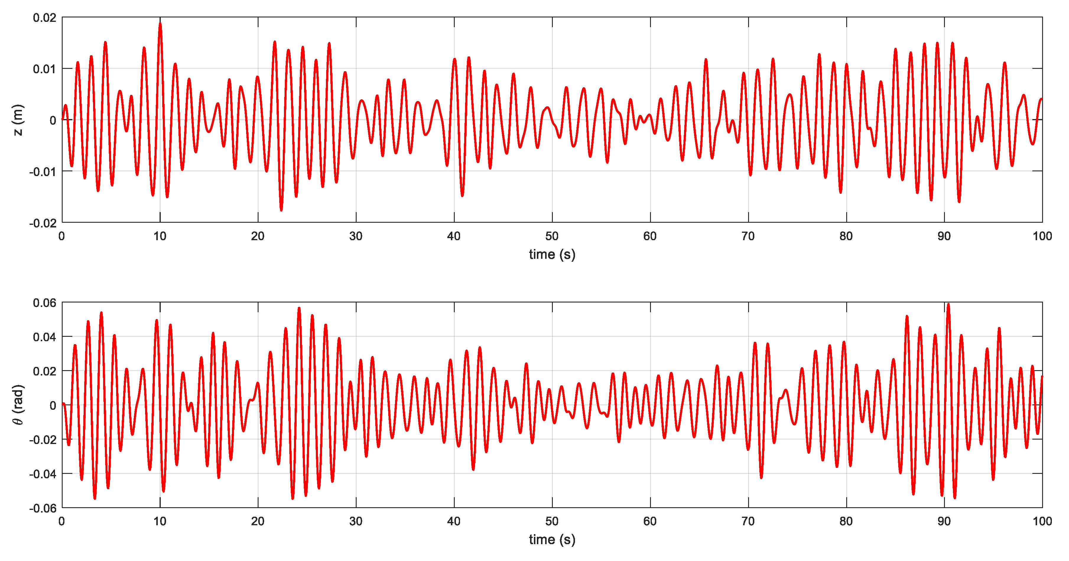
Under the initial conditions $\dot{z}=z=0,\dot{\theta }=\theta =0$ at $t=0$, Equation (9) can be solved by the fourth-order Runge-Kutta algorithm, and the integral step size is set as $\Delta t=0.05$. The simulation results are shown in Figure 3. There are 1000 samples $\left\{z(k), \theta (k)\right\},k=1,2,\cdots ,1000$, and the sampling interval is 0.1 s. The first three-fifths of the data are used for training, and the rest is used for testing the fixed-grid wavelet network. Before training the wavelet network, the data of coupled heave-pitch motions must be normalized into $[0,1]$. The original output of the system can be obtained by denormalizing the prediction results.

Equation (9) is discretized, and it gives:

$$\{\begin{array}{l}z(k)=f_1(z(k-1),z(k-2),{{\tau }^{\prime }}_3(k-1),\theta (k-1),\theta (k-2),{{\tau }^{\prime }}_5(k-1))\\ \theta (k)=f_2(z(k-1),z(k-2),{{\tau }^{\prime }}_3(k-1),\theta (k-1),\theta (k-2),{{\tau }^{\prime }}_5(k-1))\end{array}$$

(11)

where k denotes the k-th sampling instant.

It is easy to know that the six input variables in Equation (11) may be the most important. According to the prediction results, $\left\{z(k-1),z(k-2),\theta (k-1),\theta (k-2)\right\}$ are the most significant terms, and the nonlinear autoregressive (NAR) model is enough to describe the essential characteristics of the coupled heave-pitch motions in irregular waves. The structure of the fixed-grid wavelet networks is set as follows:

$$\begin{array}{cc}\hfill y_m(k)& =f_m(z(k-1),z(k-2),\theta (k-1),\theta (k-2))\hfill \\ \hfill & ={\displaystyle \sum _{i=1}^4{f}_i(x_i(k))+{\displaystyle \sum _{1\le i<j\le 4}{f}_{ij}(x_i(k),x_j(k))+e_m(k)}}\hfill \end{array}$$

(12)

where

$$y_1(k)=z(k),y_2(k)=\theta (k);x_i(k)=z(k-i)(i=1,2),\hspace{1em}{x}_i(k)=\theta (k-i)(i=3,4).$$

The functional components $f_i$ and $f_{ij}$ in Equation (12) can be fitted by the one- and two-dimensional Mexican-hat radial wavelets. The maximum number of the continuous fine-tuning is not larger than 5. The coarsest resolutions $j_1$ and the finest resolutions $j_{\max 1}$ are set to 0 and 3 in the one-dimensional radial wavelets, and the coarsest resolutions $j_2$ and the finest resolutions $j_{\max 2}$ are set to 0 and 2 in the two-dimensional radial wavelets. The sliding data window contains the data of coupled heave-pitch motions for training the wavelet model. The coarse training condition for the wavelet model of heave motion is that the other significant terms must be added in the model when ${\displaystyle {\sum }_{i}ER{R}_i<0.99}$ or $RMS{E}_{training}>0.012$, while the coarse training condition for the wavelet model of pitch motion is ${\displaystyle {\sum }_{i}ER{R}_i<0.99}$ or $RMS{E}_{training}>0.008$, where $RMS{E}_{training}$ represents the root mean square error (RMSE) of the training data. These values are determined by the trial-and-error approach, and the RMSE is defined as

$$RMSE=\sqrt{\frac{{\displaystyle {\sum }_{i=1}^N{(y_i-{\hat{y}}_i)}^2}}{N}}$$

(13)

where N represents the number of samples; $y_i$ is the sample data, and ${\hat{y}}_i$ is the estimated data by the model.

The identified model is given as

$$\{\begin{array}{l}z(k)=c_1\cdot {\psi }_{0;-1,4}^{[2]}(z(k-2),z(k-1))+c_2\cdot {\psi }_{1;-2,-2}^{[2]}(z(k-1),\theta (k-1))\\ \hspace{1em}\hspace{1em} +c_3\cdot {\psi }_{2;-1,4}^{[2]}(z(k-2),z(k-1))+c_4\cdot {\psi }_{0;1,-1}^{[2]}(z(k-2),z(k-1))\\ \hspace{1em}\hspace{1em} +c_5\cdot {\psi }_{1;2}(z(k-2))+c_6\cdot {\psi }_{2;6,2}^{[2]}(z(k-1),\theta (k-1))+c_7\cdot {\psi }_{3;0}(z(k-1))\\ \theta (k)=d_1\cdot {\psi }_{0;-1,4}^{[2]}(\theta (k-2),\theta (k-1))+d_2\cdot {\psi }_{2;4,-3}^{[2]}(\theta (k-2),\theta (k-1))\\ \hspace{1em}\hspace{1em} +d_3\cdot {\psi }_{2;-1,3}^{[2]}(\theta (k-2),\theta (k-1))+d_4\cdot {\psi }_{1;5,-2}^{[2]}(z(k-2),z(k-1))\\ \hspace{1em}\hspace{1em} +d_5\cdot {\psi }_{0;1,-1}^{[2]}(\theta (k-2),\theta (k-1))+d_6\cdot {\psi }_{2;7,-1}^{[2]}(\theta (k-2),\theta (k-1))\\ \hspace{1em}\hspace{1em} +d_7\cdot {\psi }_{0;-3,4}^{[2]}(z(k-2),z(k-1))+d_8\cdot {\psi }_{1;5,-1}^{[2]}(\theta (k-2),\theta (k-1))\end{array}$$

(14)

where the related coefficients are given in

Table 4. The coefficients in Equation (14).

Coefficient	$c_1$	$c_2$	$c_3$	$c_4$	$c_5$	$c_6$	$c_7$
Value	−34.1789	0.3242	−0.1250	−1.2824	−0.0652	−0.0677	−0.0100
Coefficient	$d_1$	$d_2$	$d_3$	$d_4$	$d_5$	$d_6$	$d_7$	$d_8$
Value	−35.6518	4.3020	−0.1215	60.1121	−0.9676	81.3790	−386.9376	12.1714

. The outputs of the identified model are inversely normalized to obtain the original system outputs.

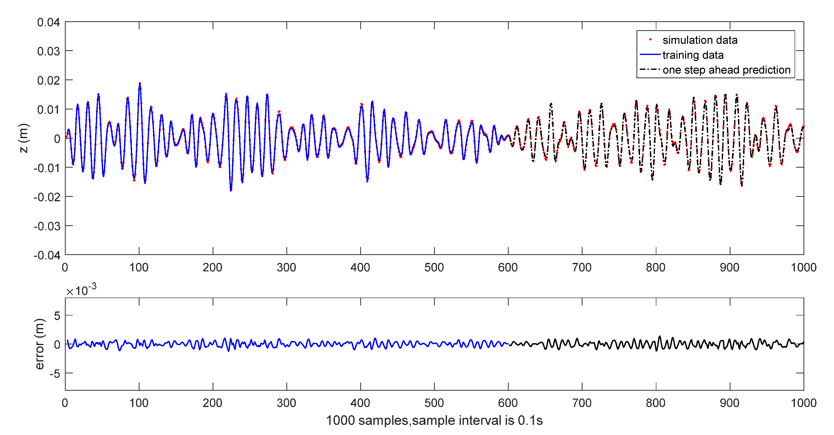
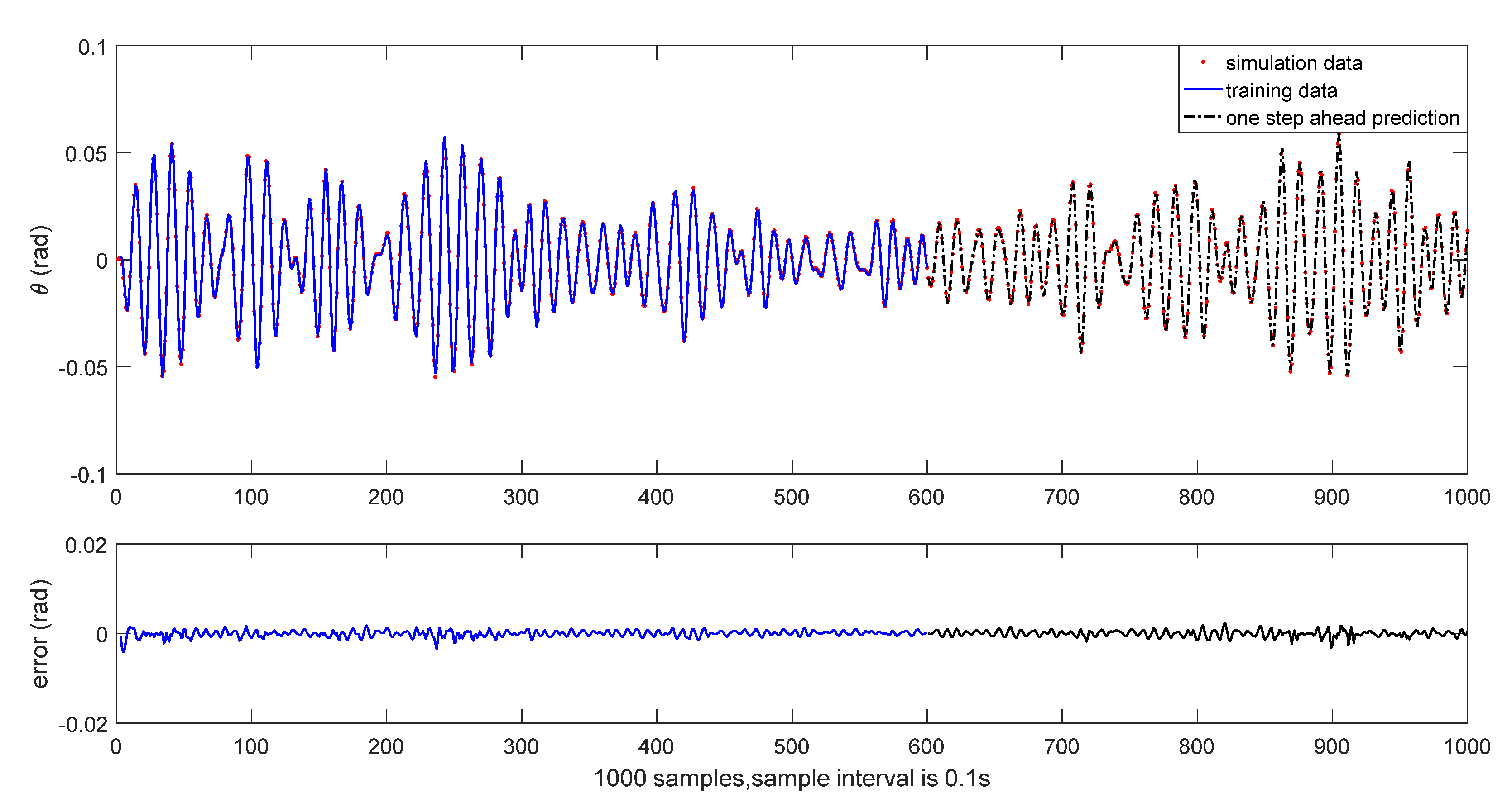
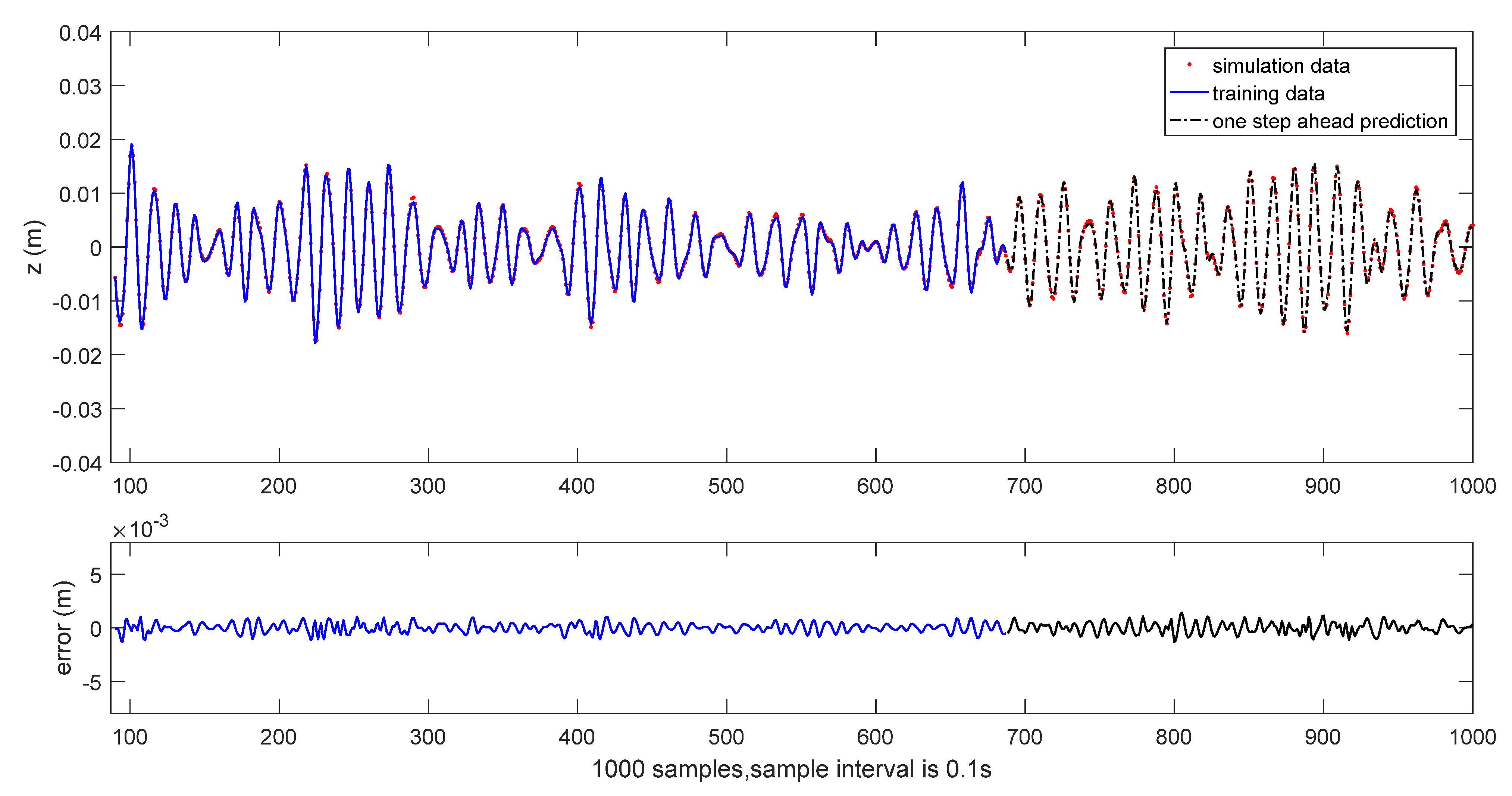
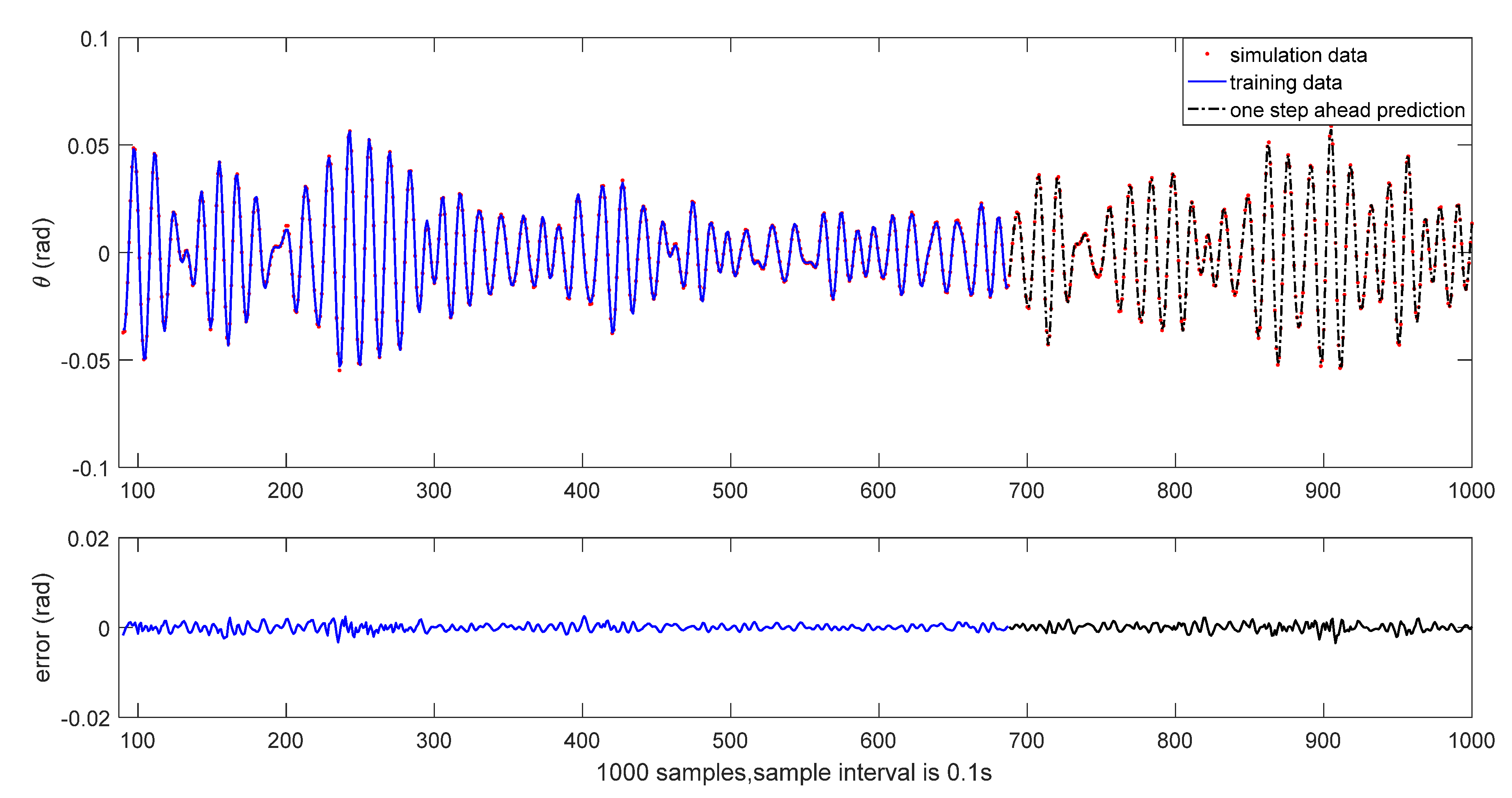
The results of initial one-step ahead prediction are depicted in Figure 4 and Figure 5, where the solid line shows the training part, and the dash line shows the testing part. The RMSE of the identified wavelet model is given in

Table 5. The RMSE of the identified wavelet model.

Motion	$RMS{E}_{training}$	$RMS{E}_{testing}$
Heave (m)	4.1442 × 10−4	4.7638 × 10−4
Pitch (rad)	7.1254 × 10−4	7.3482 × 10−4

.

The multi-steps-ahead prediction can be expressed as

$$\hat{y}(k+s)=f(\hat{z}(k+s-1),\hat{z}(k+s-2),\hat{\theta }(k+s-1),\hat{\theta }(k+s-2))$$

(15)

where s represents the prediction instant.

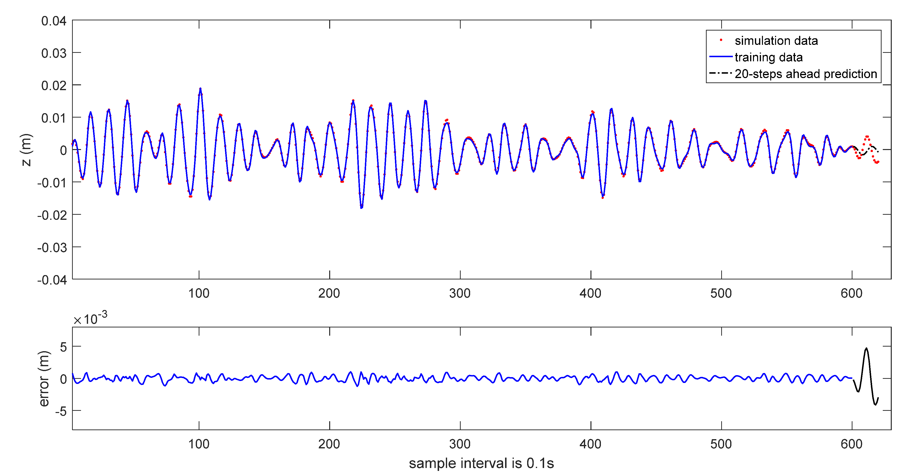
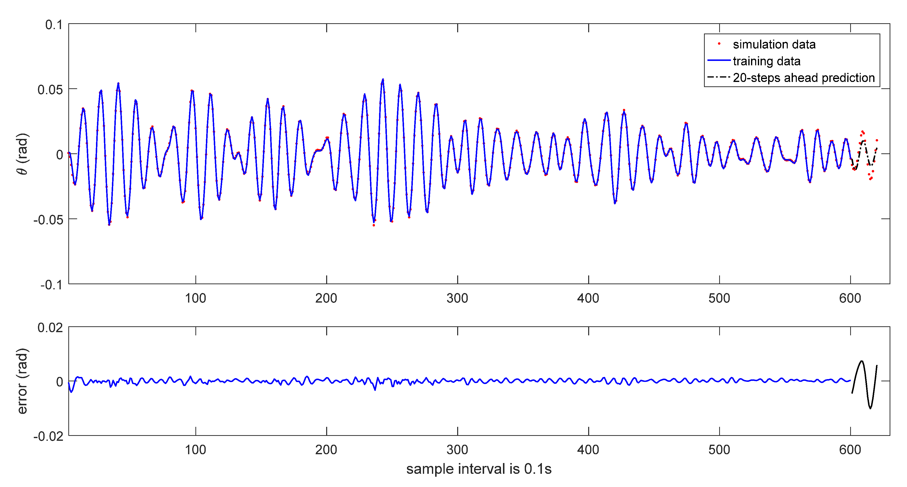
The 20-steps-ahead prediction results are depicted in Figure 6 and Figure 7. As it can be seen in these figures, the prediction performance is acceptable. Due to the accumulation of data error, the prediction performance is degraded.

When the sliding data window receives new sample data, the above modeling process will be repeated. For example, as the sliding data window moves to the sampling instant k = 687, the corresponding identified model is given as follows:

$$\{\begin{array}{l}z(k)=c_1\cdot {\psi }_{0;-1,4}^{[2]}(z(k-2),z(k-1))+c_2\cdot {\psi }_{1;-2,-2}^{[2]}(z(k-1),\theta (k-1))\\ \hspace{1em}\hspace{1em}+c_3\cdot {\psi }_{2;-1,4}^{[2]}(z(k-2),z(k-1))+c_4\cdot {\psi }_{0;1,-1}^{[2]}(z(k-2),z(k-1))\\ \hspace{1em}\hspace{1em}+c_5\cdot {\psi }_{1;2}(z(k-2))+c_6\cdot {\psi }_{2;6,2}^{[2]}(z(k-1),\theta (k-1))\\ \theta (k)=d_1\cdot {\psi }_{0;-1,4}^{[2]}(\theta (k-2),\theta (k-1))+d_2\cdot {\psi }_{0;-1,1}^{[2]}(\theta (k-2),\theta (k-1))\\ \hspace{1em}\hspace{1em}+d_3\cdot {\psi }_{0;1,1}^{[2]}(\theta (k-2),\theta (k-1))+d_4\cdot {\psi }_{1;0,2}^{[2]}(z(k-2),z(k-1))\\ \hspace{1em}\hspace{1em}+d_5\cdot {\psi }_{2;5,1}^{[2]}(\theta (k-2),\theta (k-1))+d_6\cdot {\psi }_{1;-3,4}^{[2]}(z(k-2),z(k-1))\\ \hspace{1em}\hspace{1em}+d_7\cdot {\psi }_{2;-3,5}^{[2]}(\theta (k-2),\theta (k-1))+d_8\cdot {\psi }_{2;-2,5}^{[2]}(z(k-2),z(k-1))\end{array}$$

(16)

where the related coefficients are listed in

Table 6. The coefficients in Equation (16).

Coefficient	$c_1$	$c_2$	$c_3$	$c_4$	$c_5$	$c_6$
Value	−36.0593	0.4879	−0.1297	−1.1814	−0.0633	−0.0577
Coefficient	$d_1$	$d_2$	$d_3$	$d_4$	$d_5$	$d_6$	$d_7$	$d_8$
Value	−30.9215	1.6543	0.3915	0.0211	0.0911	−151.9032	270.4504	14.9551

.

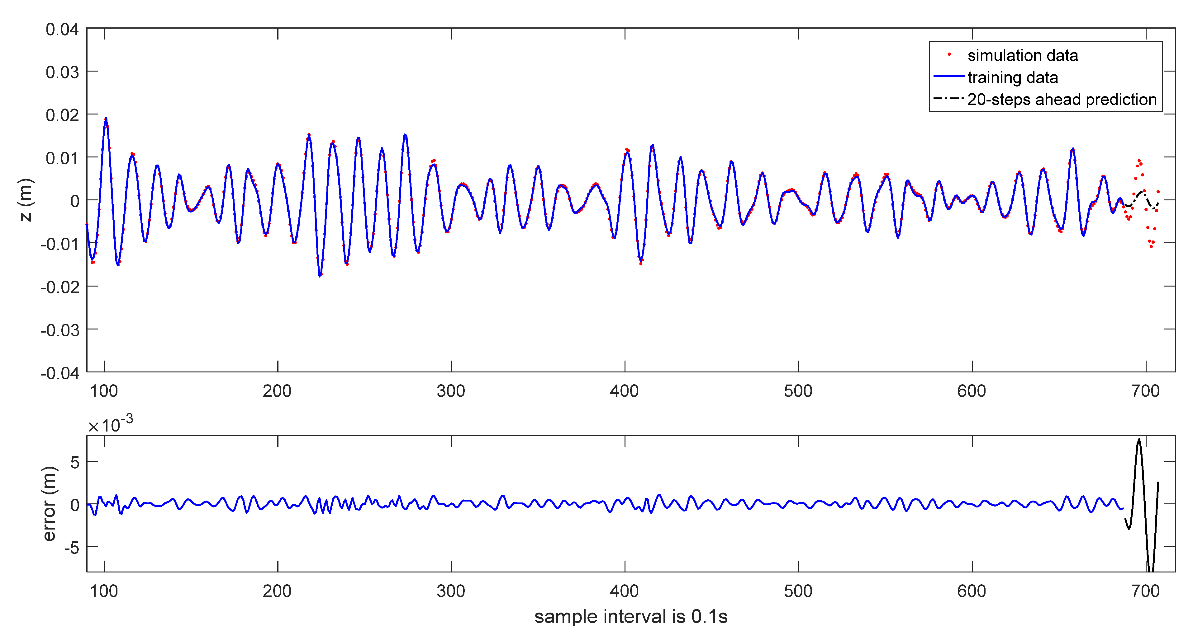
The corresponding results of one-step ahead prediction and 20-steps-ahead prediction are shown in Figure 8, Figure 9, Figure 10 and Figure 11.

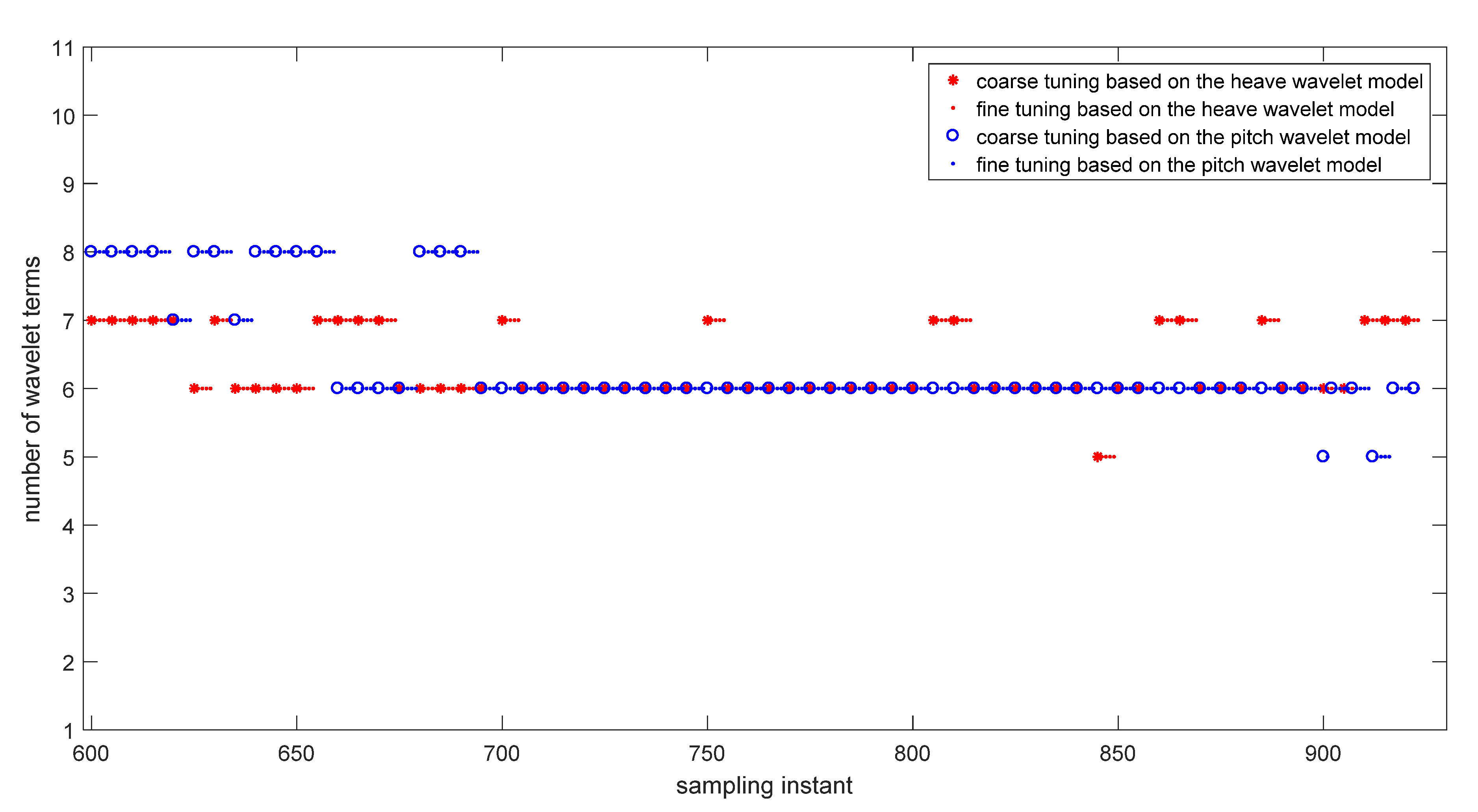
The proposed method is an online modeling method. The structure and parameters of the CFT-FGWN can change online as the sliding data window moves. When the sliding data window receives new sample data, the wavelet model can be adjusted online over time. The dynamic feature of the modeling process is shown in Figure 12. It shows that several significant wavelet terms can characterize the coupled heave-pitch motions in irregular waves very well. It is also shown clearly that the number of significant wavelet terms changes after the coarse-tuning process, and it is different for heave motion and pitch motion. The number of the continuous fine-tuning does not exceed 5, and the continuous fine-tuning can also satisfy related modeling conditions, which shows that this modeling method is effective.

The computational time of the related modeling algorithm is shown in

Table 7. Computational time with simulation data.

	Number of Coarse Tuning	Number of Fine Tuning	Computational Time of Coarse Tuning	Computational Time of Fine Tuning
Heave-FGWN	65	259	117.1726 s	1.3241 s
Pitch-FGWN	66	258	126.4073 s	1.2001 s

. Obviously, the coarse-tuning process needs more computational time than the fine-tuning process. Hence, the computational efficiency is improved by adding the continuous fine-tuning process.

It is clearly shown that the CFT-FGWN has the ability to represent the coupled heave-pitch motions in irregular waves. As a NAR modeling method, it is not necessary to measure the information of waves. This is an especially beneficial advantage, since the state of the waves is usually difficult to measure online at the open sea. As long as the past state of the coupled heave-pitch motions is obtained, the forecast model can be established online. Besides, it is easy to see that different system inputs contribute differently to the system output; thus, the influences of different system inputs can be distinguished. This is another advantage of the proposed modeling method over the conventional neural network.

4.2. Prediction Results Based on Experimental Data

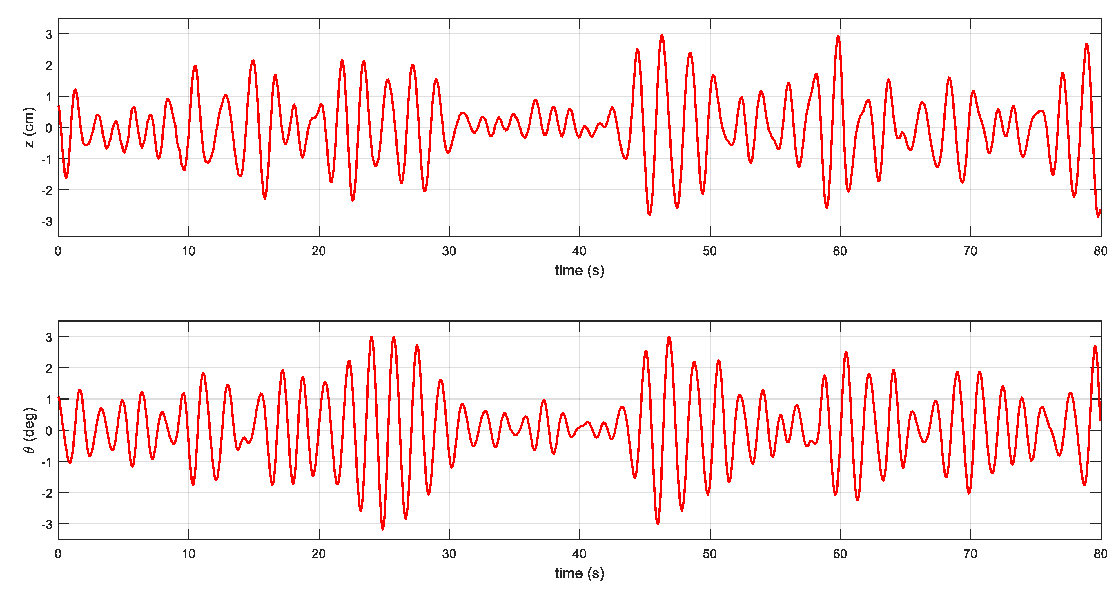
The experimental data of coupled heave-pitch motions of an FPSO model is also used to verify the effectiveness of the proposed modeling method. The experimental data are obtained from the State Key Laboratory of Ocean Engineering at Shanghai Jiao Tong University, and the principal particulars of the FPSO model are given in

Table 8. Principal particulars of the FPSO model.

Parameter	Value
Length between perpendiculars	3.71 m
Breadth	0.67 m
Depth	0.32 m
Mean draft	0.15 m
Displacement volume	0.363 m3

[31]. The JONSWAP wave spectrum is used to actuate the FPSO model. The significant wave height and the peak spectral period are 0.1852 m and 1.68 s, respectively. There are 1000 samples, and the sampling interval is 0.08 s, as shown in Figure 13. The first three-fifths of the data are used for training, and the rest is used for testing. The coarsest resolutions $j_1$ and the finest resolutions $j_{\max 1}$ are set to 0 and 3 in the one-dimensional radial wavelets, and the coarsest resolutions $j_2$ and the finest resolutions $j_{\max 2}$ are set to 0 and 2 in the two-dimensional radial wavelets. The maximum number of the continuous fine-tuning is not larger than 5. The coarse training condition for the wavelet model of heave motion is that the other significant terms must be added in the model when ${\displaystyle {\sum }_{i}ER{R}_i<0.99}$ or $RMS{E}_{training}>0.008$, while the coarse training condition for the wavelet model of pitch motion is ${\displaystyle {\sum }_{i}ER{R}_i<0.99}$ or $RMS{E}_{training}>0.006$. These values are determined by the trial-and-error approach.

The identified model is as follows:

$$\{\begin{array}{l}z(k)=c_1\cdot {\psi }_{0;-1,4}^{[2]}(z(k-2),z(k-1))+c_2\cdot {\psi }_{2;3,-2}^{[2]}(z(k-2),z(k-1))\\ \hspace{1em}\hspace{1em} +c_3\cdot {\psi }_{2;1}(z(k-2))+c_4\cdot {\psi }_{0;1,-1}^{[2]}(z(k-2),z(k-1))\\ \hspace{1em}\hspace{1em} +c_5\cdot {\psi }_{2;7,0}^{[2]}(z(k-2),z(k-1))+c_6\cdot {\psi }_{2;-3,-3}^{[2]}(z(k-2),z(k-1))\\ \hspace{1em}\hspace{1em} +c_7\cdot {\psi }_{3;10}(z(k-2))\\ \theta (k)=d_1\cdot {\psi }_{0;-1,4}^{[2]}(\theta (k-2),\theta (k-1))+d_2\cdot {\psi }_{2;3,-2}^{[2]}(\theta (k-2),\theta (k-1))\\ \hspace{1em}\hspace{1em} +d_3\cdot {\psi }_{2;1}(\theta (k-2))+d_4\cdot {\psi }_{0;1,-1}^{[2]}(\theta (k-2),\theta (k-1))\\ \hspace{1em}\hspace{1em} +d_5\cdot {\psi }_{2;6,0}^{[2]}(\theta (k-2),\theta (k-1))+d_6\cdot {\psi }_{3;-2}(\theta (k-1))\\ \hspace{1em}\hspace{1em} +d_7\cdot {\psi }_{2;5}(\theta (k-2))\end{array}$$

(17)

where the related coefficients are given in

Table 9. The coefficients in Equation (17).

Coefficient	$c_1$	$c_2$	$c_3$	$c_4$	$c_5$	$c_6$	$c_7$
Value	−37.5314	0.4640	0.0214	−1.2207	50.9184	9.0101	−0.0330
Coefficient	$d_1$	$d_2$	$d_3$	$d_4$	$d_5$	$d_6$	$d_7$
Value	−39.9604	0.3860	0.0167	−1.1384	1.8944	0.0368	0.0239

. The outputs of the identified model are inversely normalized to obtain the original system outputs.

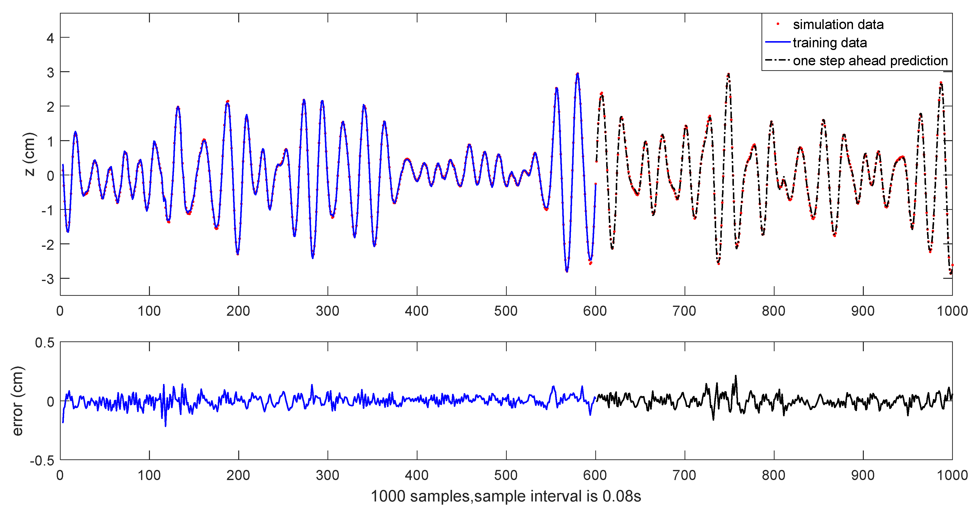
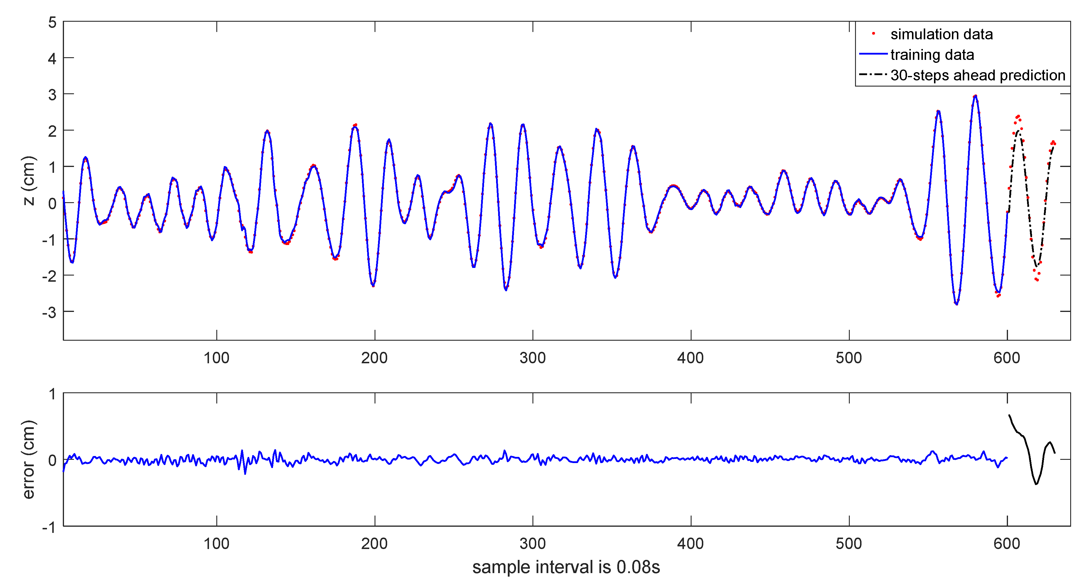
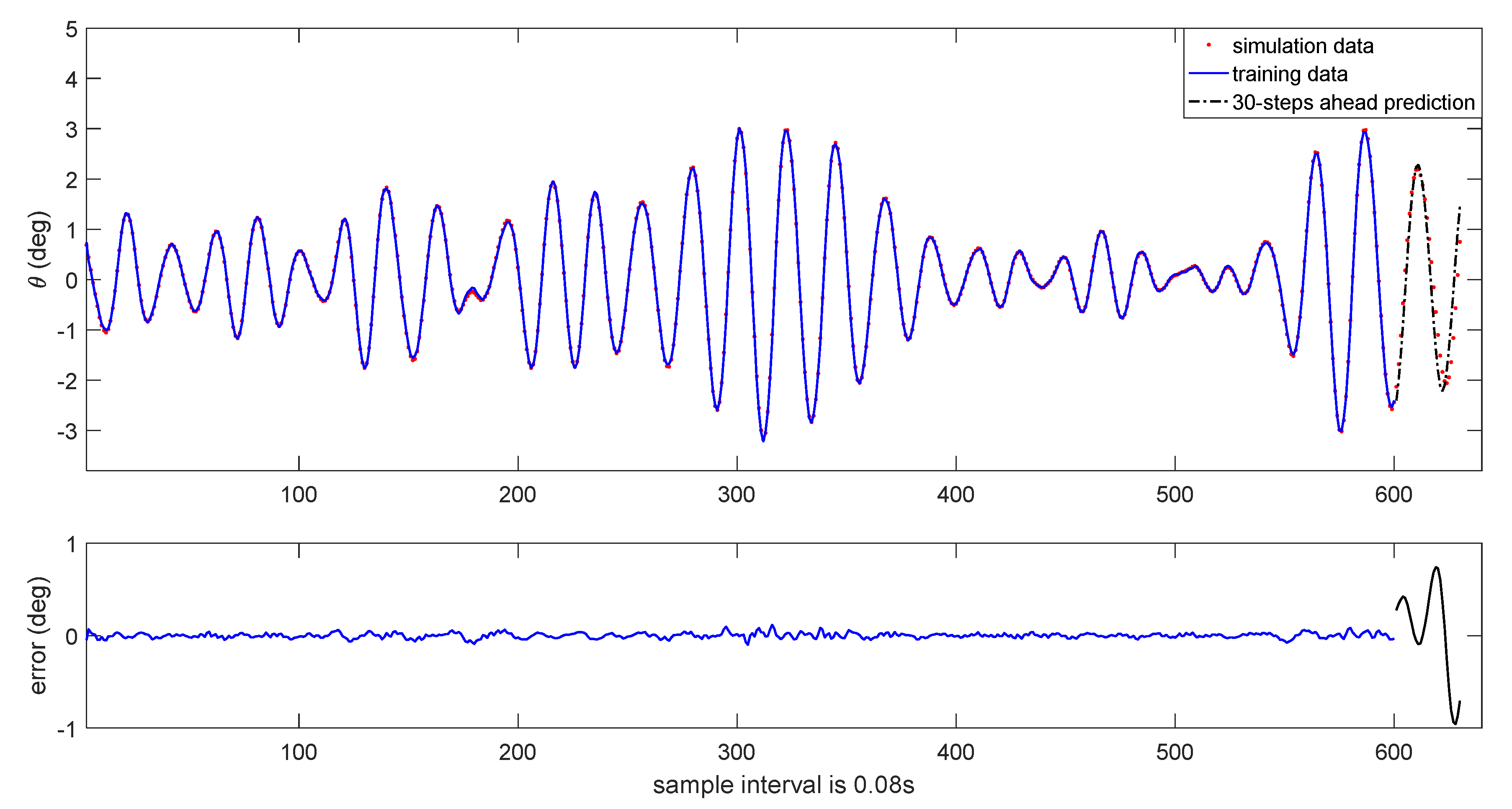
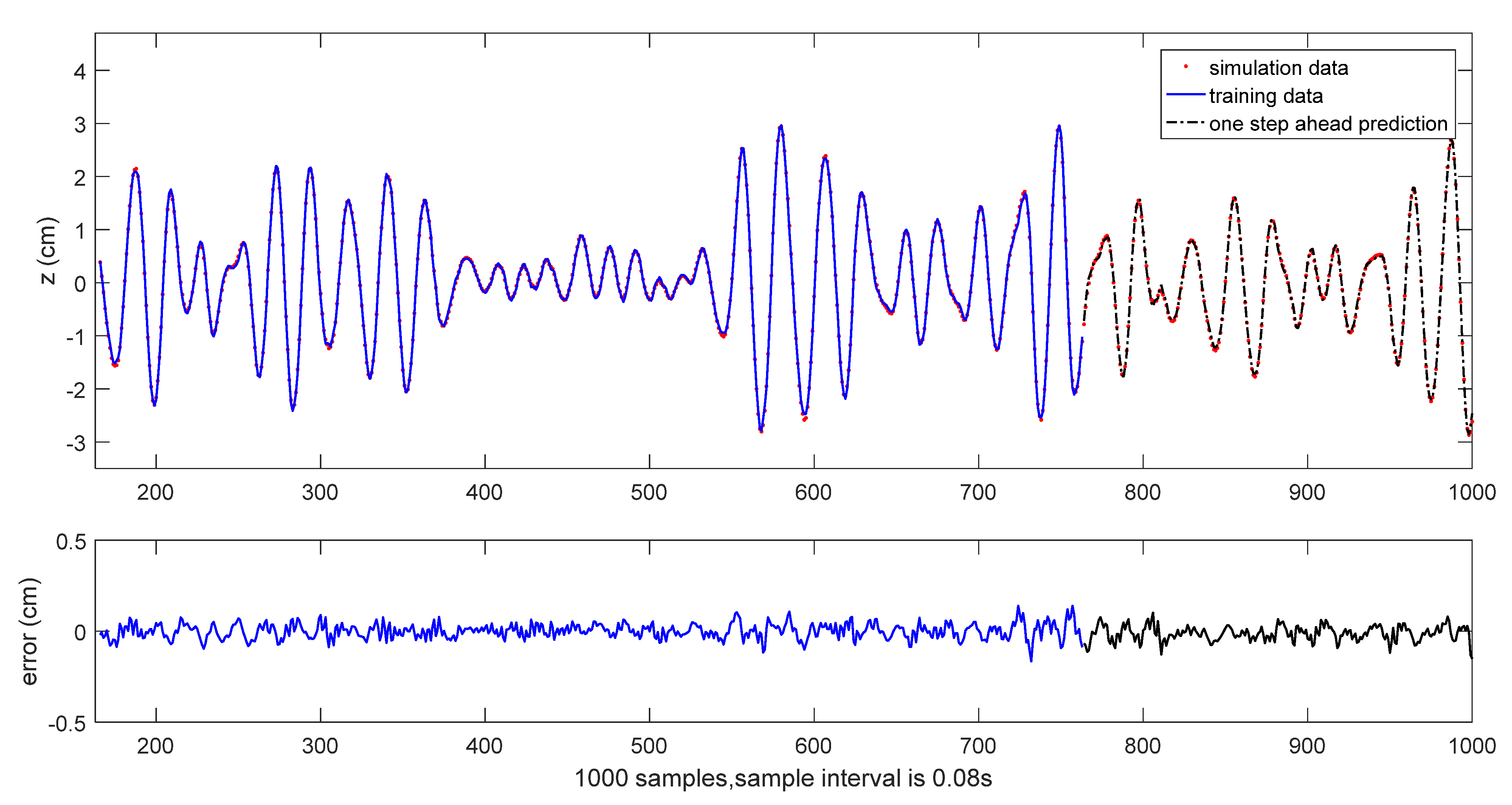
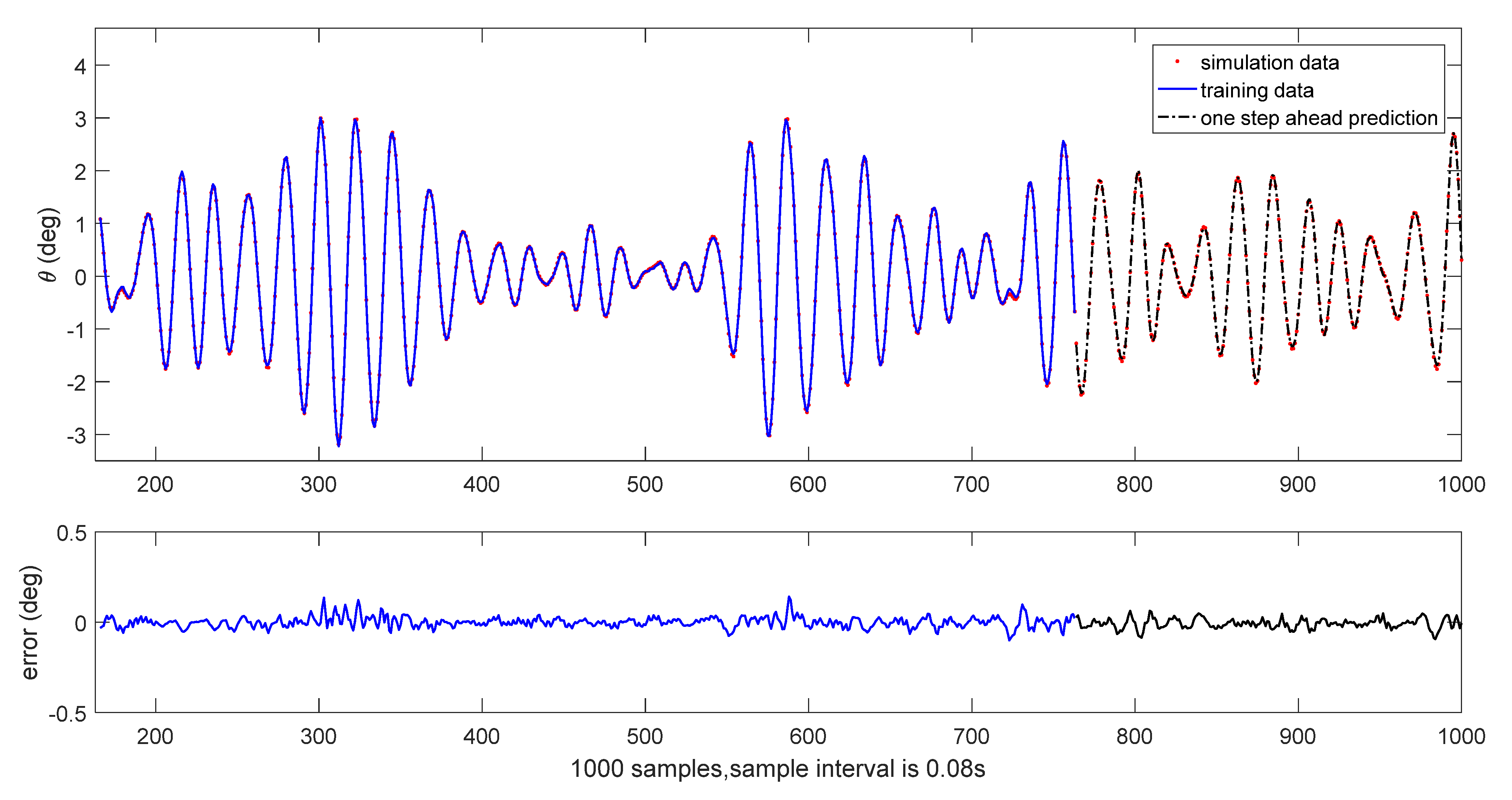
The results of initial one-step ahead prediction are depicted in Figure 14 and Figure 15. The results of 30-steps-ahead prediction are depicted in Figure 16 and Figure 17. It can be seen that the prediction performance is satisfactory.

As the sliding data window continues to move, it receives new data and the model can be adjusted online. For example, when the sliding data window receives the data at the sampling instant k = 763, the corresponding model is identified as follows:

$$\{\begin{array}{l}z(k)=c_1\cdot {\psi }_{0;-1,4}^{[2]}(z(k-2),z(k-1))+c_2\cdot {\psi }_{2;3,-2}^{[2]}(z(k-2),z(k-1))\\ \hspace{1em}\hspace{1em} +c_3\cdot {\psi }_{2;1}(z(k-2))+c_4\cdot {\psi }_{0;1,-1}^{[2]}(z(k-2),z(k-1))\\ \hspace{1em}\hspace{1em} +c_5\cdot {\psi }_{2;7,0}^{[2]}(z(k-2),z(k-1))+c_6\cdot {\psi }_{1;2,-3}^{[2]}(z(k-2),z(k-1))\\ \hspace{1em}\hspace{1em} +c_7\cdot {\psi }_{1;3,3}^{[2]}(z(k-2),z(k-1))\\ \theta (k)=d_1\cdot {\psi }_{0;-1,4}^{[2]}(\theta (k-2),\theta (k-1))+d_2\cdot {\psi }_{2;3,-2}^{[2]}(\theta (k-2),\theta (k-1))\\ \hspace{1em}\hspace{1em} +d_3\cdot {\psi }_{2;1}(\theta (k-2))+d_4\cdot {\psi }_{0;1,-1}^{[2]}(\theta (k-2),\theta (k-1))\\ \hspace{1em}\hspace{1em} +d_5\cdot {\psi }_{2;6,0}^{[2]}(\theta (k-2),\theta (k-1))+d_6\cdot {\psi }_{3;-2}(\theta (k-1))\\ \hspace{1em}\hspace{1em} +d_7\cdot {\psi }_{0;4,-2}^{[2]}(z(k-2),z(k-1))\end{array}$$

(18)

where the related coefficients are given in

Table 10. The coefficients in Equation (18).

Coefficient	$c_1$	$c_2$	$c_3$	$c_4$	$c_5$	$c_6$	$c_7$
Value	−36.5040	−0.1151	0.0192	−1.4192	42.8903	1.9687	0.0656
Coefficient	$d_1$	$d_2$	$d_3$	$d_4$	$d_5$	$d_6$	$d_7$
Value	−39.2299	0.4820	0.0175	−1.0484	2.2043	0.0422	−10.6728

.

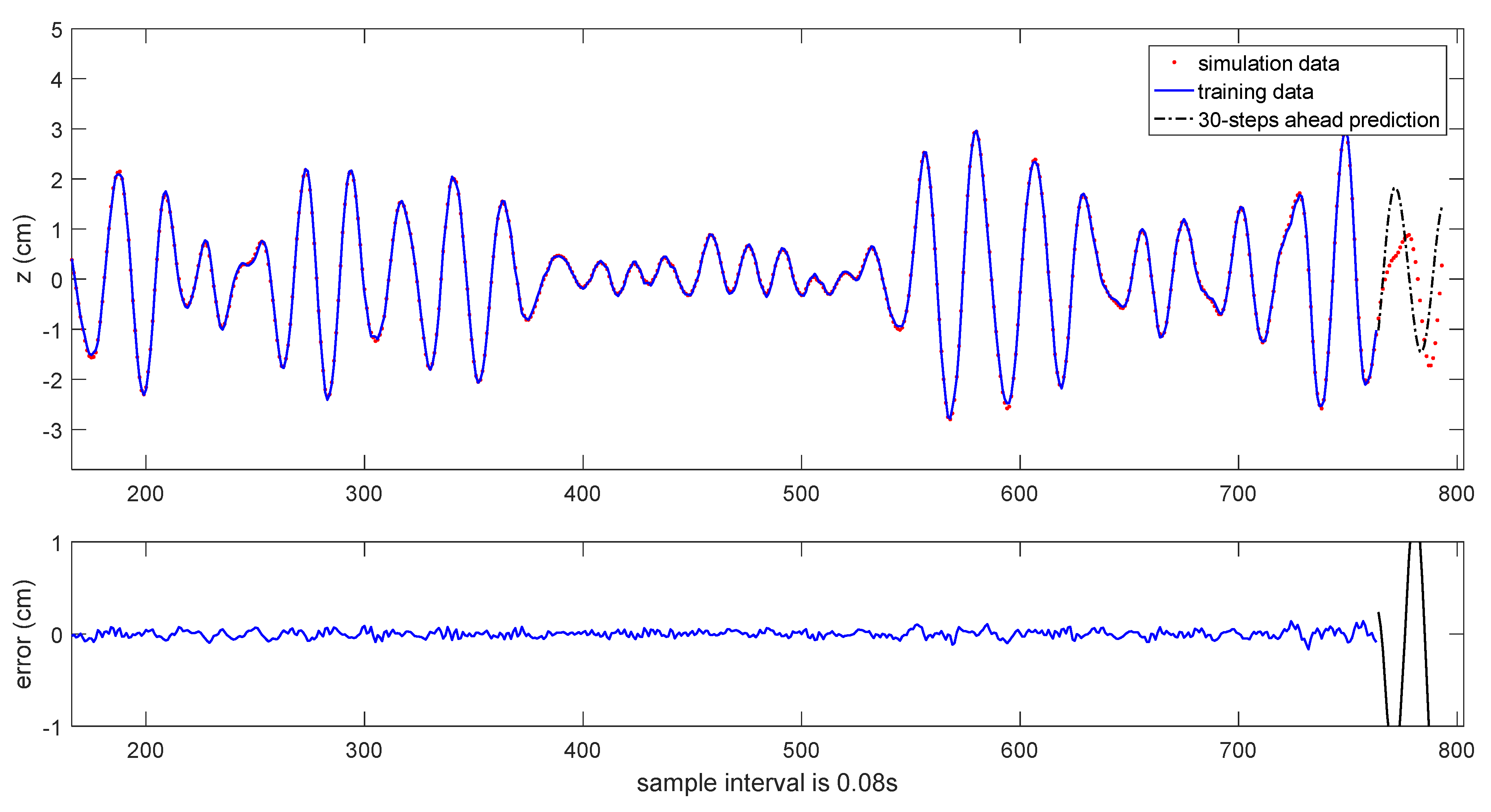
The results of the one-step ahead prediction and the 30-steps-ahead prediction are shown in Figure 18, Figure 19, Figure 20 and Figure 21.

The structure of the CFT-FGWN can be adjusted online over time, and the change process is shown in Figure 22. It can be seen clearly that several significant wavelet terms can characterize the coupled heave-pitch motions in irregular waves, which shows that the CFT-FGWN has a strong nonlinear fitting ability.

The computational time of the related modeling algorithm is given in

Table 11. Computational time with experimental data.

	Number of Coarse Tuning	Number of Fine Tuning	Computational Time of Coarse Tuning	Computational Time of Fine Tuning
Heave-FGWN	67	267	171.4563 s	1.4676 s
Pitch-FGWN	67	267	182.2069 s	1.3377 s

. It can be seen that the fine-tuning process takes less computational time than the coarse-tuning process. The computational efficiency is improved significantly due to the continuous fine-tuning process.

5. Conclusions

The CFT-FGWN is used for online modeling ship’s coupled heave-pitch motions in irregular waves. The effectiveness of the modeling method is verified by applying it based on the simulation data and the real experimental data. The prediction results using the established wavelet model showed that this online modeling method is not only feasible, but also has high computational efficiency, and several significant wavelet terms can capture the intrinsic nonlinear dynamics of the coupled heave-pitch motions, which indicates that the modeling method has the ability to give a good prediction of the coupled heave-pitch motions of a ship in irregular waves, and it can be applied to MIMO systems.

Based on the simulation results, the continuous fine-tuning process requires less computational time, which increases the computational efficiency largely. A heuristic method will be considered to determine the number of continuous fine-tuning in the future work.

References

1. Huang, B.G.; Zou, Z.J. Short-term prediction of ship pitching motion based on artificial neural networks. In Proceedings of the 35th International Conference on Ocean, Offshore and Arctic Engineering, Busan, Korea, 19–24 June 2016. [Google Scholar]
2. Triantafyllou, M.; Athans, M. Real time estimation of the heaving and pitching motions of a ship using a Kalman filter. In OCEANS 81; Marine Technology Society: Boston, MA, USA, 16–18 September 1981; pp. 1090–1095. [Google Scholar]
3. Triantafyllou, M.; Bodson, M.; Athans, M. Real time estimation of ship motions using Kalman filtering techniques. IEEE J. Ocean. Eng. 1983, 8, 9–20. [Google Scholar] [CrossRef] [Green Version]
4. Khan, A.; Marion, K.E.; Bil, C.; Simic, M. Motion prediction for ship-based autonomous air vehicle operations. Intell. Interact. Multimed. Syst. Serv. 2016, 2016, 323–333. [Google Scholar]
5. Li, G.Y.; Kawan, B.; Wang, H.; Zhang, H.X. Neural-network-based modeling and analysis for time series prediction of ship motion. Ship Technol. Res. 2017, 64, 30–39. [Google Scholar] [CrossRef] [Green Version]
6. De Masi, G.; Gaggiotti, F.; Bruschi, R.; Venturi, M. Ship motion prediction by radial basis neural networks. In Proceedings of the 2011 IEEE Workshop on Hybrid Intelligent Models and Applications, Paris, France, 11–15 April 2011; pp. 28–32. [Google Scholar]
7. Duan, W.Y.; Huang, L.M.; Han, Y.; Zhang, Y.H.; Huang, S. A hybrid AR-EMD-SVR model for the short-term prediction of nonlinear and non-stationary ship motion. J. Zhejiang Univ.-Sci. A 2015, 16, 562–576. [Google Scholar] [CrossRef] [Green Version]
8. Liu, S.; Yang, Z. Online prediction of ship rolling based on varying parameters LSSVM. J. Ship Mech. 2012, 16, 1024–1034. [Google Scholar]
9. Xu, C.Z.; Zou, Z.J. Online prediction of ship roll motion in waves based on auto-moving gird search-least square support vector machine. Math. Probl. Eng. 2021, 2021, 2760517. [Google Scholar]
10. De Masi, G.; Bruschi, R.; Gaggiotti, F. Short term vessel motion forecasting based on wavelet neural network for wave feed-forward dynamic positioning. In Proceedings of the 22nd International Offshore and Polar Engineering Conference, Rhodes, Greece, 17–22 June 2012; pp. 915–919. [Google Scholar]
11. Wang, Y.C.; Liu, F.M.; Fu, H.X. Ship rolling motion prediction based on wavelet neural network. Appl. Mech. Mater. 2012, 190, 724–728. [Google Scholar] [CrossRef]
12. Suhermi, N.; Suhartono Prastyo, D.D.; Ali, B. Roll motion prediction using a hybrid deep learning and ARIMA model. Procedia Comput. Sci. 2018, 144, 251–258. [Google Scholar] [CrossRef]
13. Su, Y.; Lin, J.; Zhao, D.; Guo, C.; Wang, C.; Guo, H. Real-time prediction of large-scale ship model vertical acceleration based on recurrent neural network. J. Mar. Sci. Eng. 2020, 8, 777. [Google Scholar] [CrossRef]
14. Hu, X.; Zhang, B.; Tang, G. Research on ship motion prediction algorithm based on dual-pass Long Short-Term Memory neural network. IEEE Access 2021, 9, 28429–28438. [Google Scholar] [CrossRef]
15. Zhang, W.; Wu, P.; Peng, Y.; Liu, D. Roll motion prediction of unmanned surface vehicle based on coupled CNN and LSTM. Future Internet 2019, 11, 243. [Google Scholar] [CrossRef] [Green Version]
16. Kecman, V. Learning and Soft Computing: Support Vector Machines, Neural Networks, and Fuzzy Logic Models; MIT Press: Cambridge, MA, USA, 2001. [Google Scholar]
17. Haddara, M.R.; Xu, J. On the identification of ship coupled heave-pitch motions using neural networks. Ocean. Eng. 1998, 26, 381–400. [Google Scholar] [CrossRef]
18. Yin, J.C.; Zou, Z.J.; Xu, F. On-line prediction of ship roll motion during maneuvering using sequential learning RBF neural networks. Ocean. Eng. 2013, 61, 139–147. [Google Scholar] [CrossRef]
19. Hou, X.R.; Zou, Z.J.; Xu, F. SVR-based parameter identification of coupled heave-pitch motion equations in regular waves. In Proceedings of the 26th International Ocean and Polar Engineering Conference, Rhodes, Greece, 26 June–1 July 2016. [Google Scholar]
20. Huang, B.G.; Zou, Z.J.; Ding, W.W. Online prediction of ship roll motion based on a coarse and fine tuning fixed grid wavelet network. Ocean. Eng. 2018, 160, 425–437. [Google Scholar] [CrossRef]
21. Huang, B.G.; Zou, Z.J. Online prediction of ship roll motion in irregular waves using a fixed grid wavelet network. J. Ship Mech. 2020, 24, 693–705. [Google Scholar]
22. Billings, S.A.; Wei, H.L. A new class of wavelet networks for nonlinear system identification. IEEE Trans. Neural Netw. 2005, 16, 862–874. [Google Scholar] [CrossRef] [PubMed] [Green Version]
23. Chen, Z. Fitting multivariate regression functions by interaction spline models. J. R. Stat. Soc. Ser. B (Methodol.) 1993, 55, 473–491. [Google Scholar] [CrossRef]
24. Wei, H.L.; Billings, S.A. Long term prediction of non-linear time series using multiresolution wavelet models. Int. J. Control 2006, 79, 569–580. [Google Scholar] [CrossRef]
25. Billings, S.A.; Korenberg, M.J.; Chen, S. Identification of non-linear output-affine systems using an orthogonal least-squares algorithm. Int. J. Syst. Sci. 1988, 19, 1559–1568. [Google Scholar] [CrossRef]
26. Chen, S.; Billings, S.A.; Luo, W. Orthogonal least squares methods and their application to non-linear system identification. Int. J. Control 1989, 50, 1873–1896. [Google Scholar] [CrossRef]
27. Gentleman, W.M. Least squares computations by Givens transformations without square roots. IMA J. Appl. Math. 1973, 12, 329–336. [Google Scholar] [CrossRef]
28. Luo, W.; Billings, S.A. Adaptive model selection and estimation for nonlinear systems using a sliding data window. Signal Process. 1995, 46, 179–202. [Google Scholar] [CrossRef]
29. Bhattacharyya, R. Dynamics of Marine Vehicles; John Wiley & Sons Inc.: New York, NY, USA, 1978. [Google Scholar]
30. Xu, J. Identification of Ship Coupled Heave and Pitch Motions Using Neural Networks; Memorial University of Newfoundland: St. John’s, NL, Canada, 1997. [Google Scholar]
31. Hou, X.R.; Zou, Z.J. Parameter identification of nonlinear roll motion equation for floating structures in irregular waves. Appl. Ocean. Res. 2016, 55, 66–75. [Google Scholar] [CrossRef]
Figure 1. Flow chart of the coarse-tuning and fine-tuning algorithm for the coupled heave-pitch motions.
Jmse 09 00989 g001
Figure 2. The JONSWAP wave spectrum and related irregular waves.
Jmse 09 00989 g002
Figure 3. The coupled heave-pitch motions of the R-Class Icebreaker model in irregular waves.
Jmse 09 00989 g003
Figure 4. The one-step-ahead prediction of heave motion in irregular waves for the R-Class Icebreaker model.
Jmse 09 00989 g004
Figure 5. The one-step-ahead prediction of pitch motion in irregular waves for the R-Class Icebreaker model.
Jmse 09 00989 g005
Figure 6. The 20-steps-ahead prediction of heave motion in irregular waves for the R-Class Icebreaker model.
Jmse 09 00989 g006
Figure 7. The 20-steps-ahead prediction of pitch motion in irregular waves for the R-Class Icebreaker model.
Jmse 09 00989 g007
Figure 8. The one-step-ahead prediction of heave motion in irregular waves at the instant k = 687 for the R-Class Icebreaker model.
Jmse 09 00989 g008
Figure 9. The one-step-ahead prediction of pitch motion in irregular waves at the instant k = 687 for the R-Class Icebreaker model.
Jmse 09 00989 g009
Figure 10. The 20-steps-ahead prediction of heave motion in irregular waves at the instant k = 687 for the R-Class Icebreaker model.
Jmse 09 00989 g010
Figure 11. The 20-steps-ahead prediction of pitch motion in irregular waves at the instant k = 687 for the R-Class Icebreaker model.
Jmse 09 00989 g011
Figure 12. The structure of the CFT-FGWN changing over time based on the simulation data.
Jmse 09 00989 g012
Figure 13. The coupled heave-pitch motions of the FPSO model in irregular waves.
Jmse 09 00989 g013
Figure 14. The one-step ahead prediction of heave motion in irregular waves for the FPSO model.
Jmse 09 00989 g014
Figure 15. The one-step ahead prediction of pitch motion in irregular waves for the FPSO model.
Jmse 09 00989 g015
Figure 16. The 30-steps-ahead prediction of heave motion in irregular waves for the FPSO model.
Jmse 09 00989 g016
Figure 17. The 30-steps-ahead prediction of pitch motion in irregular waves for the FPSO model.
Jmse 09 00989 g017
Figure 18. The one-step ahead prediction of heave motion in irregular waves at the instant k = 763 for the FPSO model.
Jmse 09 00989 g018
Figure 19. The one-step ahead prediction of pitch motion in irregular waves at the instant k = 763 for the FPSO model.
Jmse 09 00989 g019
Figure 20. The 30-steps-ahead prediction of heave motion in irregular waves at the instant k = 763 for the FPSO model.
Jmse 09 00989 g020
Figure 21. The 30-steps-ahead prediction of pitch motion in irregular waves at the instant k = 763 for the FPSO model.
Jmse 09 00989 g021
Figure 22. The structure of the CFT-FGWN changing over time based on the experimental data.
Jmse 09 00989 g022