A Cost-Effective Approach to the Risk Reduction of Cable Fault Triggered by Laying Repeaters of Fiber-Optic Submarine Cable Systems in Deep-Sea

Abstract

Long-distance submarine cable systems, such as the transoceanic system, generally consist of a series of cables and repeaters. Repeater units are spaced at regular intervals to boost the attenuated optical signal and presently contain optical amplifiers in a pressure vessel made of copper alloy. Since the repeater unit is more massive than the cable, it pulls the cable catenary locally toward the seabed. In the 1990s, several studies numerically simulated cable behavior in the water and showed that the seabed slack runs short, and the seabed cable tension increases just before the repeater reaches the seabed. Therefore, it has been pointed out that an unarmored cable with a polyethylene sheath can be easily damaged. However, no reports have been published regarding the actual situation of cable faults related to the laying of repeaters. This study quantitatively analyzes the mechanism of cable damage related to the laying of repeaters, based on experiments, simulations, maintenance records, and a comparative analysis between the simulation results and actual cable faults. Cost-effective methods to mitigate cable faults triggered by laying a repeater in the deep sea are also explored to ensure mechanical stability during the design lifetime.

1. Introduction

The first submarine cable, in the 1850s, crossed the English Channel, between England and France, to enable telegraphic communication [1]. Cables in the 19th century were composed of iron wire wrapped around natural insulation material, such as Gutta-Percha, which surrounded single or multi-strand copper wires at the core. The communication path was between the copper core wire and the earth [2]. The transmission data rate was limited to 15 words per minute by the considerable distortion of the signal’s waveform, due to the inherent capacitance of the cable [1]. By 2016, the fiber-optic submarine cable system (hereafter referred to as the system), which is not related to cable capacitance, had evolved to a mind-boggling 10 Tbps (terabits per second) of bandwidth per fiber [3]. Without these cables, the internet would quickly hit gridlock, and social activities that depend heavily on digitalized information would be severely restricted. Therefore, a highly reliable system is strongly demanded by society. A system supported by state-of-the-art technology may be subject to complete network outages, due to human activity or natural factors, until the completion of repairs. The system is vulnerable at points where the infrastructure passes through geographic “chokepoints,” such as the Luzon Strait, between Taiwan and the Philippines, which are susceptible to earthquakes, particularly between Japan and Southeast Asia [4]. In the East China Sea, off the coast of China, systems are frequently damaged by anchors from fishing activities or shipping industries [5].

Another cause of system failures, in addition to those mentioned above, is the method of laying repeaters. Since the 1950s, when the coaxial cable system was developed to enable the use of telephones, the periodic strengthening of signals transmitted over a significant distance has been necessary [1]. Therefore, repeaters are arranged in-line, at regular intervals, between landing stations. Initially, with the use of the coaxial cable, the great difficulty encountered during the installation of a repeater was supporting its weight in the catenary to the seabed, and it would cause excess strain on the cable. A method was needed to relieve this additional strain. One solution was to attach parachutes to repeaters when they were deployed [6]. The theory is that the parachute will open in the water column and bear some of the repeater weight during its descent to the seabed. After a more durable cable was developed in 1968, the usage of parachutes was abandoned [6].

The need to understand cable behavior in the water began to be recognized, and the theory for calculating the kinematic behavior of a cable in the water was developed in the latter half of the 1950s [7]. However, since this theory did not consider repeaters, studies to develop mathematical solutions were conducted in the 1960s. In the 1980s, with the improvement of computer performance, numerical simulations of cable behavior in the water were applied [8,9].

In fiber-optic submarine cable systems, there is a significant difference in the weights of the repeater and the cable, and each element behaves differently in the water. Therefore, the cable length is shorter than the seabed distance in some areas just before the repeater reaches the seabed (potentially several kilometers in deep water, as explained in Section 3.4). As a result, the cable becomes stressed and drags along the seabed. Due to the design trend of unarmored cables with a thinner polyethylene insulation layer, the weight of the cable has become lighter. As a result, the difference between the weights of cables and repeaters has continued to increase, which increases the risk of a cable fault. Therefore, the drag range of the cable is more likely to cause faults. The above risk was pointed out in several studies, based on simulation results [8,9]. However, to date, there have been no reports of cable faults associated with repeater installations anywhere in the world (within the scope of our literature search).

For system reliability, it is crucial to ensure not only the manufacturing quality of the submergible equipment but also the overall reliability, including the construction method. An objective for the reliability associated with the production of the system is the need for fewer than three repairs within 25 years of the system design lifetime [10]. The construction quality of the system is not standardized because natural factors make it difficult to standardize the mechanical durability of installed systems. The cause of system failures has been studied since 2004 [11]. Reference [12] analyzed data on submarine cable faults caused by external damage from 1960 to 2005. The causes were broadly classified into fisheries, shipping, human activities, and natural disasters, such as earthquakes, submarine landslides, and a component of submergible equipment.

Although the causes of the cable faults investigated in this study have been included among natural factors in previous studies [11,12], the occurrence of cable faults caused by repeater installation remains unknown. Therefore, this study was focused mainly on obtaining an accurate understanding of the fault situation triggered by repeater installation at great water depths. The purpose of this research work is to improve the mechanical reliability of the system in a cost-effective manner by optimizing the laying of repeaters to mitigate cable faults that occur in the cable drag range.

In order to clarify the causes of the cable faults investigated in this study, the paper is divided into six sections. In Section 1, the background is presented by reviewing previous studies, and the purpose of this research is explained. Section 2 presents the physical parameters and specifications of the repeater and cables of the system, the experiment for the sinking speed of the repeaters, the calculation of the sinking speed of cables, and the actual situation of repeater placement intervals. In Section 3, the definition of slack, an outline of the numerical simulation, the simulation analysis of cable behavior with the repeater, and a comparison of the simulation results in different repeater laying conditions are described. In Section 4, the results, regarding cable faults associated with repeater installation, are analyzed, based on the system dynamics obtained from the simulation results in Section 3, and the geographical locations where cable faults tend to occur are presented. Section 5 discusses reducing the risk of cable faults by shortening the cable drag range, based on the shipboard cable tension when the repeater reaches the seabed, and cost-effective measures, aimed at mitigating cable faults caused by repeater installation, are proposed. Finally, the main conclusions of this study are presented in Section 6.

2. The Mechanical Construction of Repeaters and Cables and Their Sinking Speeds

Understanding the critical elements of the system, the repeater, and the physical components of the cable is the basis for analysis and suggestions. The mechanical construction and sinking speed of the repeaters and cables are assessed in this section.

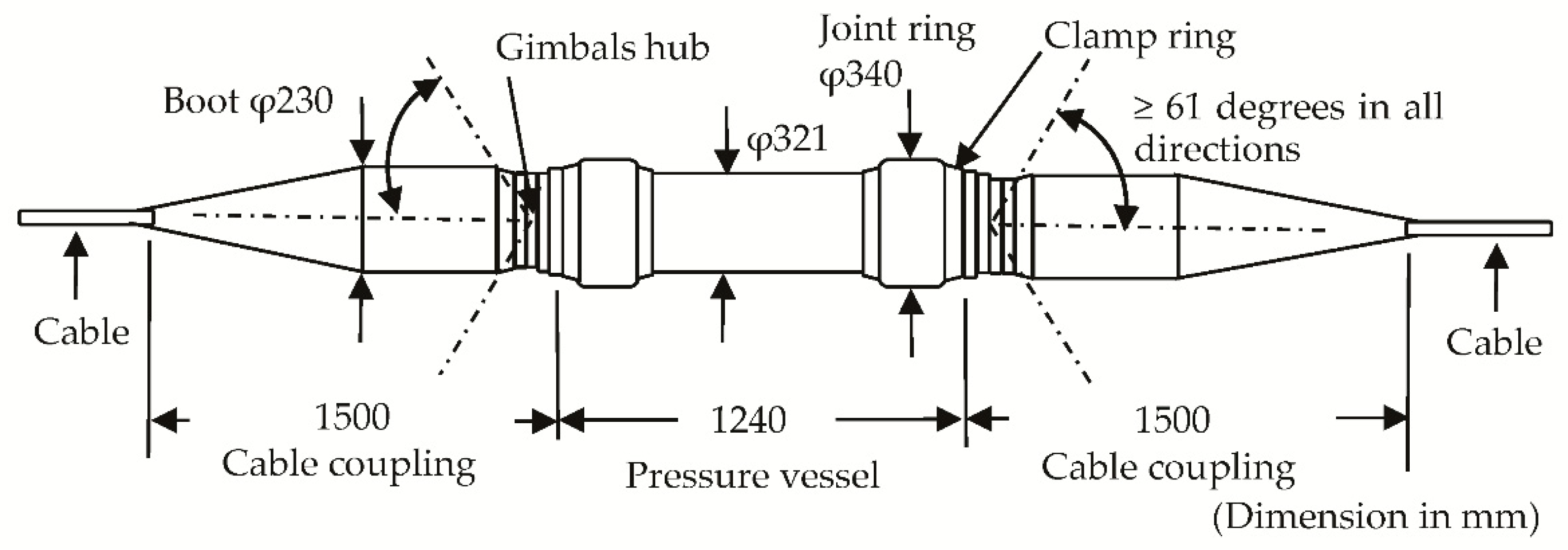
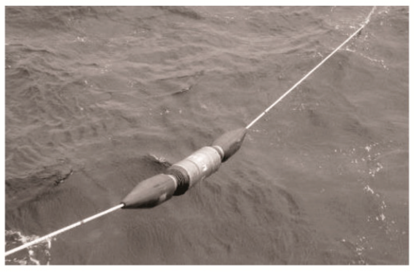
2.1. Repeater

Figure 1 shows the basic overall construction of a repeater unit for a fiber-optic submarine cable system [13] used in Japan, since the 1990s. The repeater unit consists of a pressure vessel, which houses electronics in the center and a cable coupling at each end. The required physical design must withstand water pressure, vibration, heat dissipation, and chemical erosion by the seawater, at a maximum water depth of 8000 m. Therefore, the pressure vessel is cylindrical, and the material is beryllium copper (BeCu) alloy, which has excellent corrosion resistance, mechanical strength, and thermal conductivity. BeCu alloys typically contain 98% copper, 1.7% beryllium, and 0.3% cobalt [14].

The cylinder structure connects to a conical coupling that bends freely by a gimbal mechanism at each end to facilitate passage while winding around the curved surface of the laying gear, such as a drum cable engine or sheave on the cable ship. The overall weight, including cable terminations in the air and water, is approximately 550 kgf and 440 kgf, respectively.

Figure 2 shows a repeater being laid from a cable ship. The repeaters generate the optical signals after attenuation by propagation through each span along the cable.

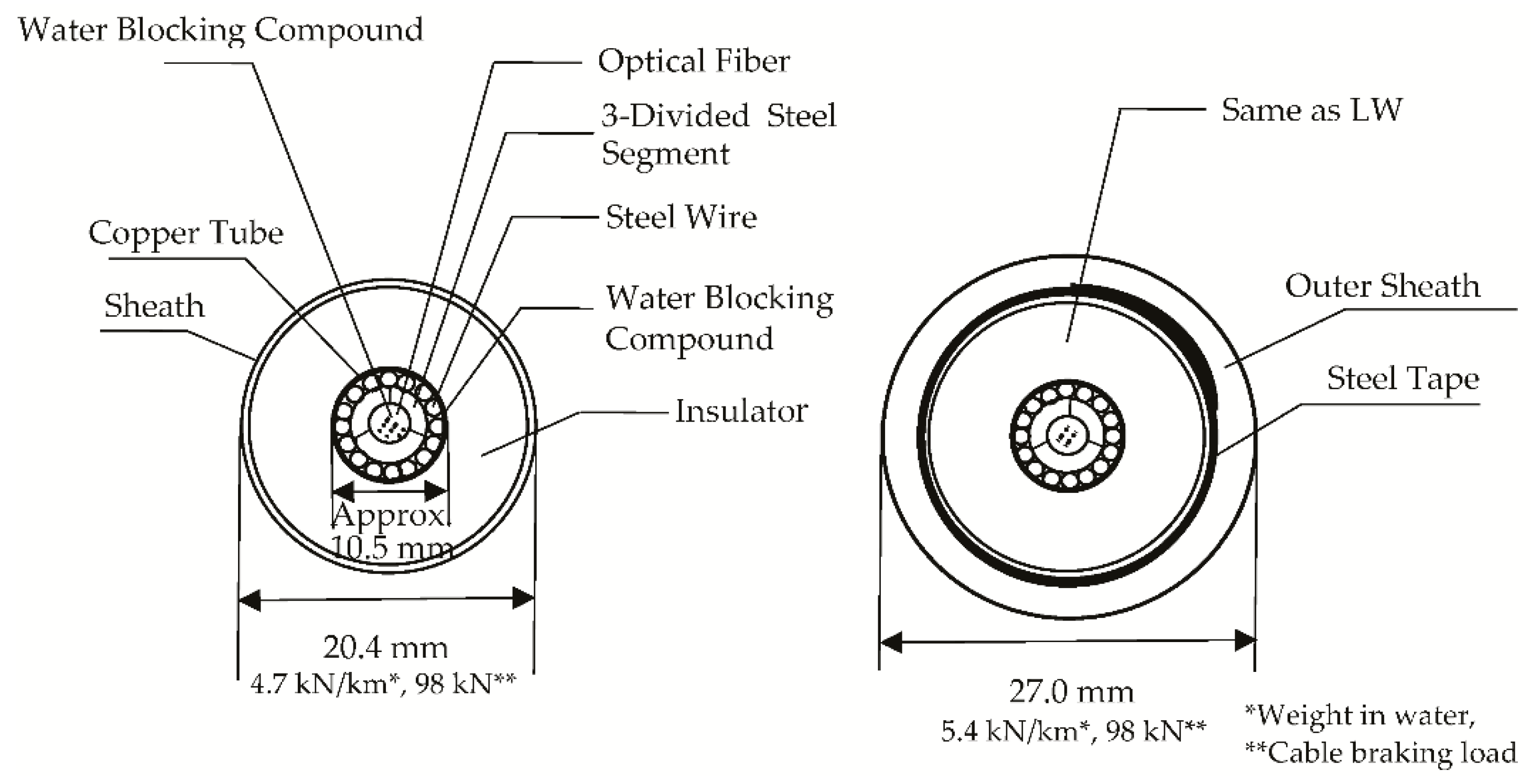
2.2. Cables

Fiber-optic submarine cables for repeated systems mainly consist of light guides made of silica-based glass and power-feeding copper conductors, which supply electric power to submergible plants. Among commercially available cables, two typical cables are lightweight and lightweight screened cables. The basic fiber-optic submarine cable is an unarmored LW (lightweight) cable. The cross-section of the LW cable [15] is shown in Figure 3 (left). The LW cable has a polyethylene sheath to electrically insulate the copper tube from the seawater and can be applied to water depths up to 8000 m.

The construction of the LWS (lightweight screened) cable is the same as that of the LW cable, but with an added steel tape layer and an additional polyethylene sheath. The cross-section of the LWS cable [15] is shown in Figure 3 (right). The LWS cable is designed to resist large fish bites, abrasion during deployment, external damage while in service, and water depths up to 6000 m.

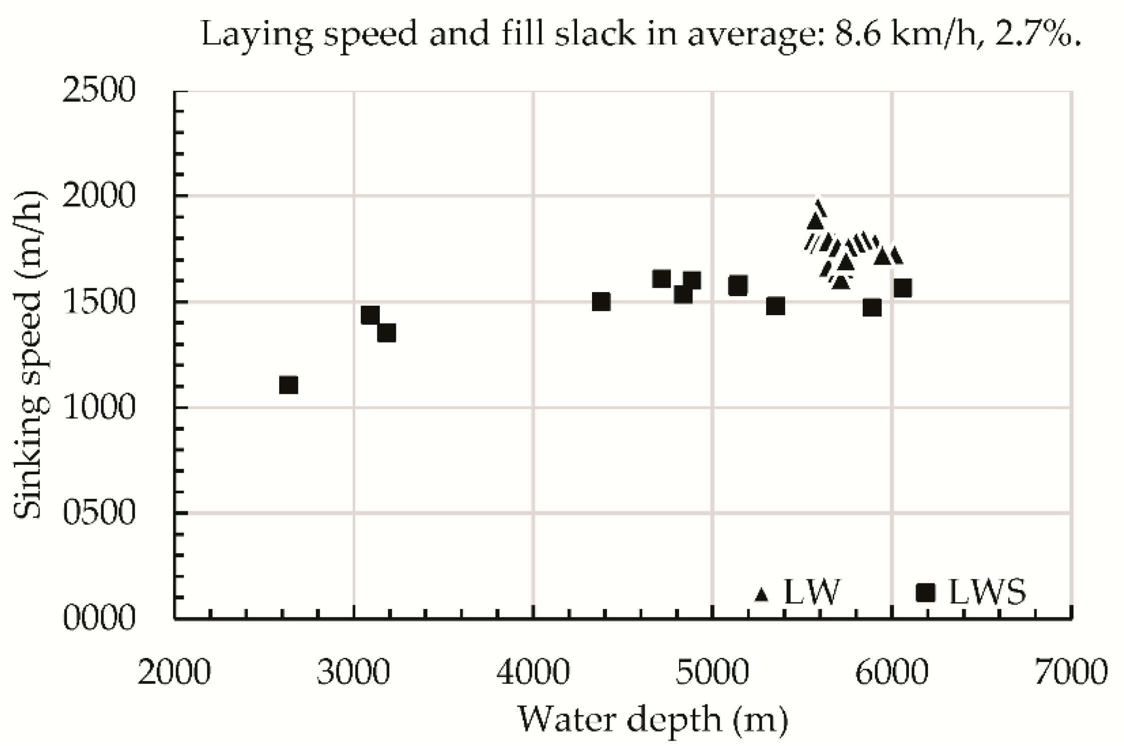
2.3. Comparison of Sinking Speeds of Repeater and Cables

2.3.1. Method for a Physical Experiment to Confirm the Sinking Speed of the Repeater with Cables

The system is laid directly on the seabed, while repeaters are laid in conjunction with laying the cable and are inseparable from that process. The sinking speed of the repeater was experimentally obtained using a series of system installation stages consisting of LW and LWS cables at both ends. The procedure is as follows:

• Step 1: Record the position of the laying ship and the time at the beginning of the repeater laying process.
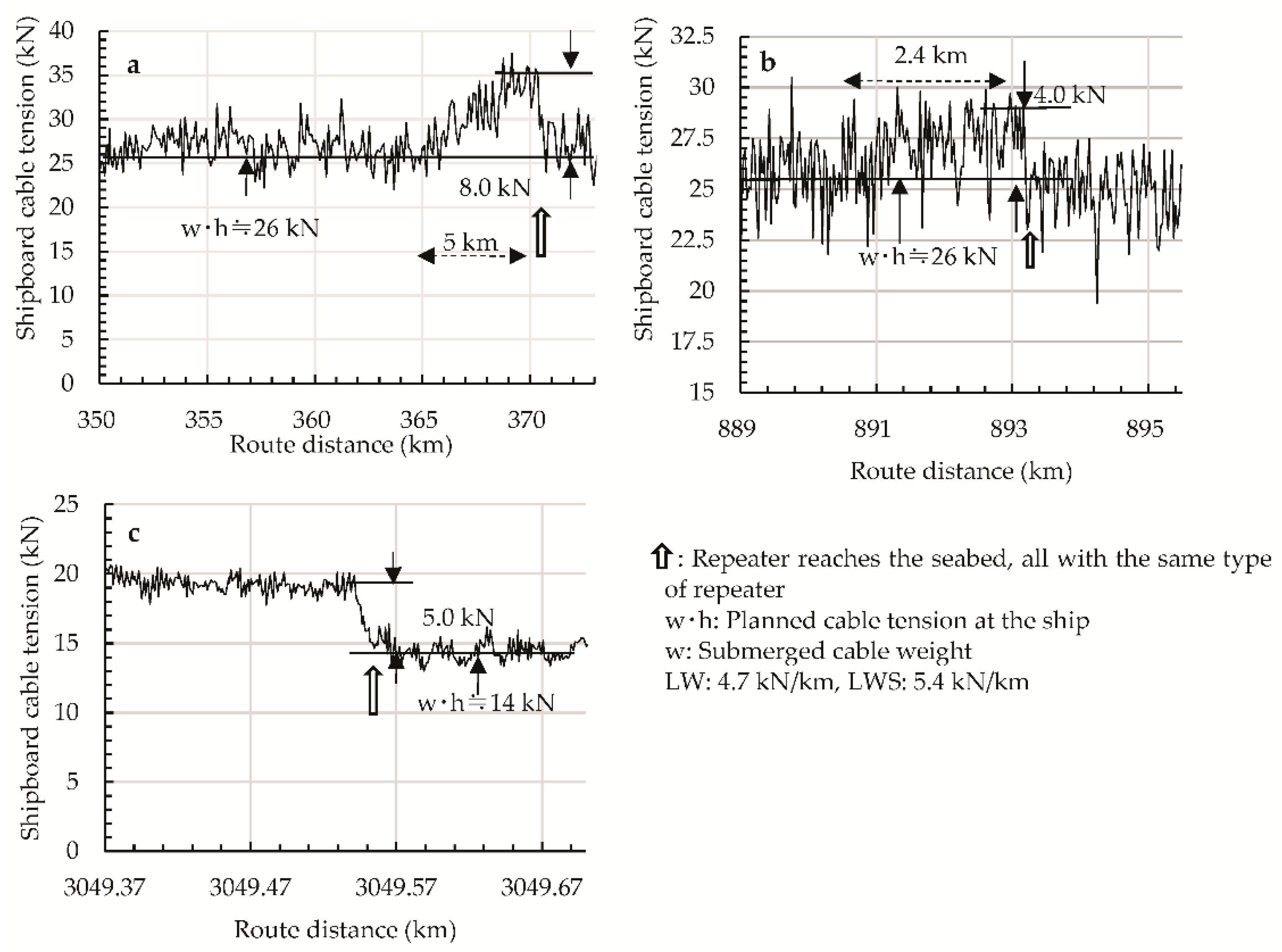
• Step 2: Based on the change in the cable tension on the ship (details are explained in Section 3), record the time when the repeater reaches the seabed, the estimated seabed position, and the water depth from the bathymetry data (obtained by the route survey before the system design).
• Step 3: Calculate the sinking speed from the time difference between Steps 1 and 2.

Figure 4 shows the experimental results for the sinking speed of the same type of repeater with cables on both ends. For the repeater with LW cables, the sinking speed is distributed mainly around 1750 m/h, at water depths between 5800 and 6000 m; for the repeater with LWS cables, the speed is distributed around the center of 1500 m/h, in water depths ranging from 2600 to 6000 m. The difference in the water depth range between the two cable types is due to differences in cable design specifications, as described in Section 2.2.

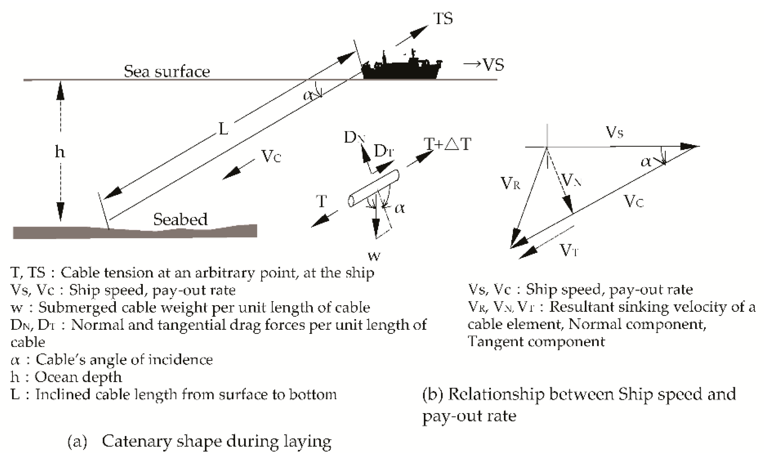
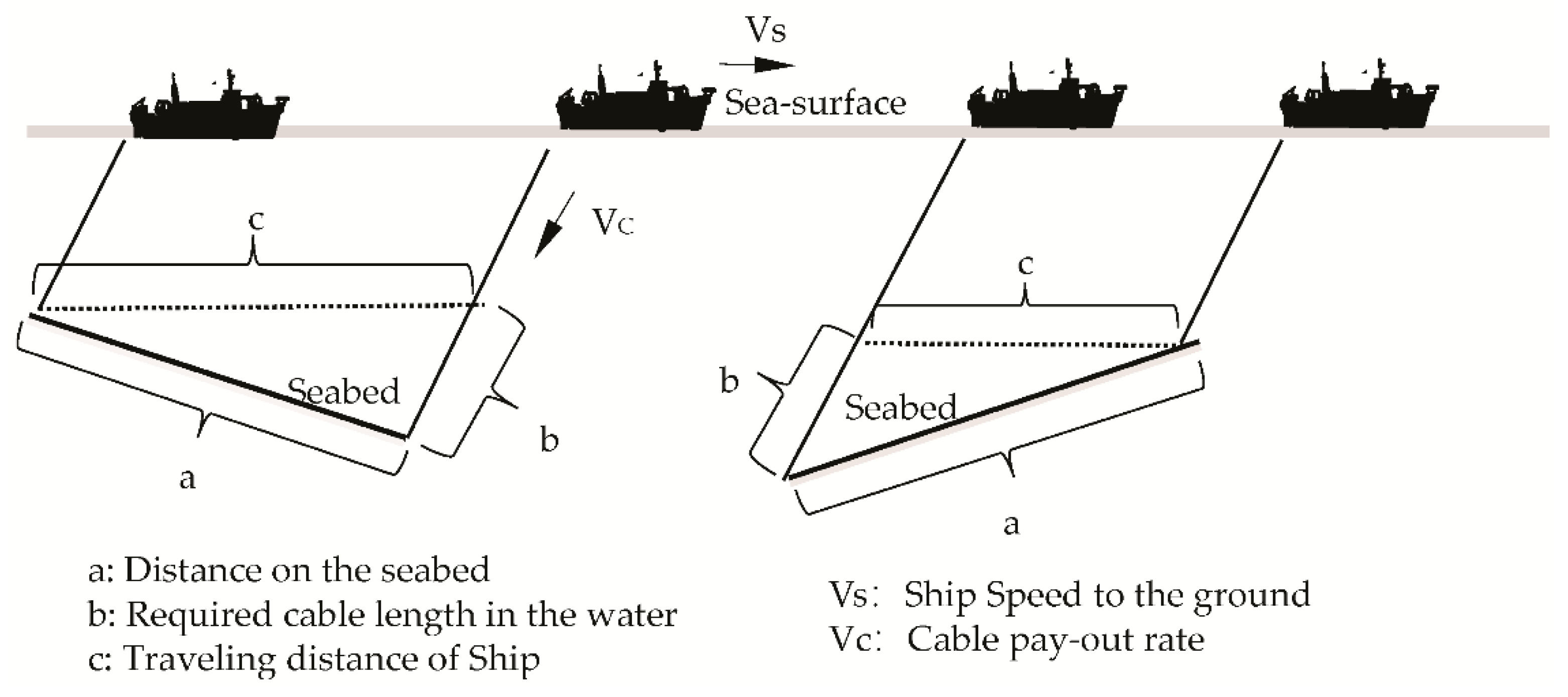
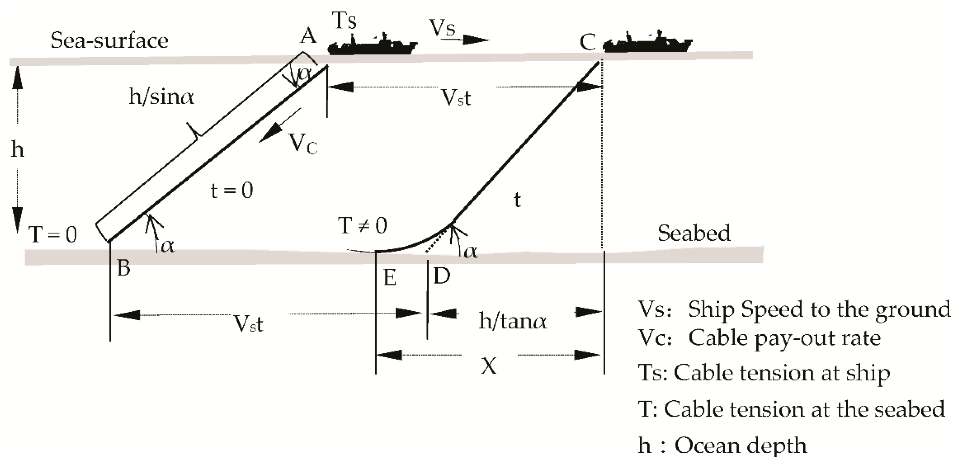
2.3.2. Calculation of Transversal Sinking Speed of Cables

In this section, to obtain the transversal sinking speed of cables, the cable configuration is analyzed and discussed based on the dynamics of a two-dimensional stationary model [7]. The forces acting on the cable during the laying process are shown in Figure 5.

At a sufficiently slow speed, the resistance to a fluid flow around an immersed body varies as the square of the fluid velocity; therefore, the relationship between normal unit drag force, D_N, and other parameters is usually determined by Equation (1) [7]:

D_N = C_D ρ V_N² d/2

(1)

where C_D is the hydrodynamic coefficient of the cable drag, ρ is the density of seawater, V_N is the standard component of the resultant sinking velocity, and d is the cable diameter.

In the case of transverse or normal flow around the cable, the variation of D_N, with the square of the relative transverse velocity, gives (V_N/U_S)² = D_N/w [7]. D_N is calculated using Equation (2).

Here, U_S is defined as the terminal velocity attained by a straight, horizontal cable sinking in water.

D_N = w (V_N/U_S)²

(2)

Substituting for D_N in Equation (1), Equation (3) is obtained.

U_S = (2 w/C_D ρ d)^1/2

(3)

Here, the quantity (2 w/C_D ρ d)^1/2 is defined as the hydrodynamic constant H for a given cable. Thus, the transverse sinking velocity U_S is identical to the hydrodynamic constant H, as shown in Equation (4):

U_S = H

(4)

where U_S is in knots.

Table 1. Parameters used in calculation and calculated results.

Cable Parameter and Physical Constants Required for Calculation	LW	LWS
d: Diameter (mm)	20.4	27.0
w: Weight in water (kN/km)	4.7	5.4
CD: Hydrodynamics coefficient of the cable drag [16]	2.5
ρ: Density of seawater (kg·sec2/m4) [16]	102
Calculation result
H: Hydrodynamic constant (degree·knot)	47.8	44.6
Us: Transverse sinking velocity (m/h)	1544	1441

shows the cable parameters and physical constants used in the calculation and the calculation results for each cable type.

The values of H and U_S for LW and LWS cables are then calculated based on the mechanical specifications, shown in Section 2.2.

2.3.3. Comparative Sinking Speeds between Repeater and Cables

Table 2. Comparative sinking speed between repeater and cables.

Targets	Sinking Speed (m/h)	Ratio of Repeater Sinking Speed to Cable (%)
Repeater with LW	1750	+13.34
LW (Calculation)	1544	---
Repeater with LWS	1500	+4.09
LWS (Calculation)	1441	---

shows the sinking speed of the repeater with the cables, the sinking speed of the cables, and the ratio of the sinking speed of the repeater to that of the cable, based on experiments in Section 2.3.1 and calculations in Section 2.3.2. The comparison shows that the repeater’s sinking speed is strongly dependent on the cable construction, increasing by 13.34% for LW and 4.09% for LWS relative to the cable sinking speed. The reason for this difference is that the sinking speed of the LW cable is much faster than that of the LWS cable.

2.4. Repeater Spacing

The repeater spacing of the system was investigated because it affects the number of laid repeaters and is, therefore, related to the risk of cable faults. To understand repeater placement intervals, we surveyed several transpacific systems commercialized from 1989 to 2016. The distance between repeaters varies, depending on the transmission technology used. The spacing is about 40–150 km, centered on about 60 km.

3. Numerical Simulation of Cable Behavior in the Water

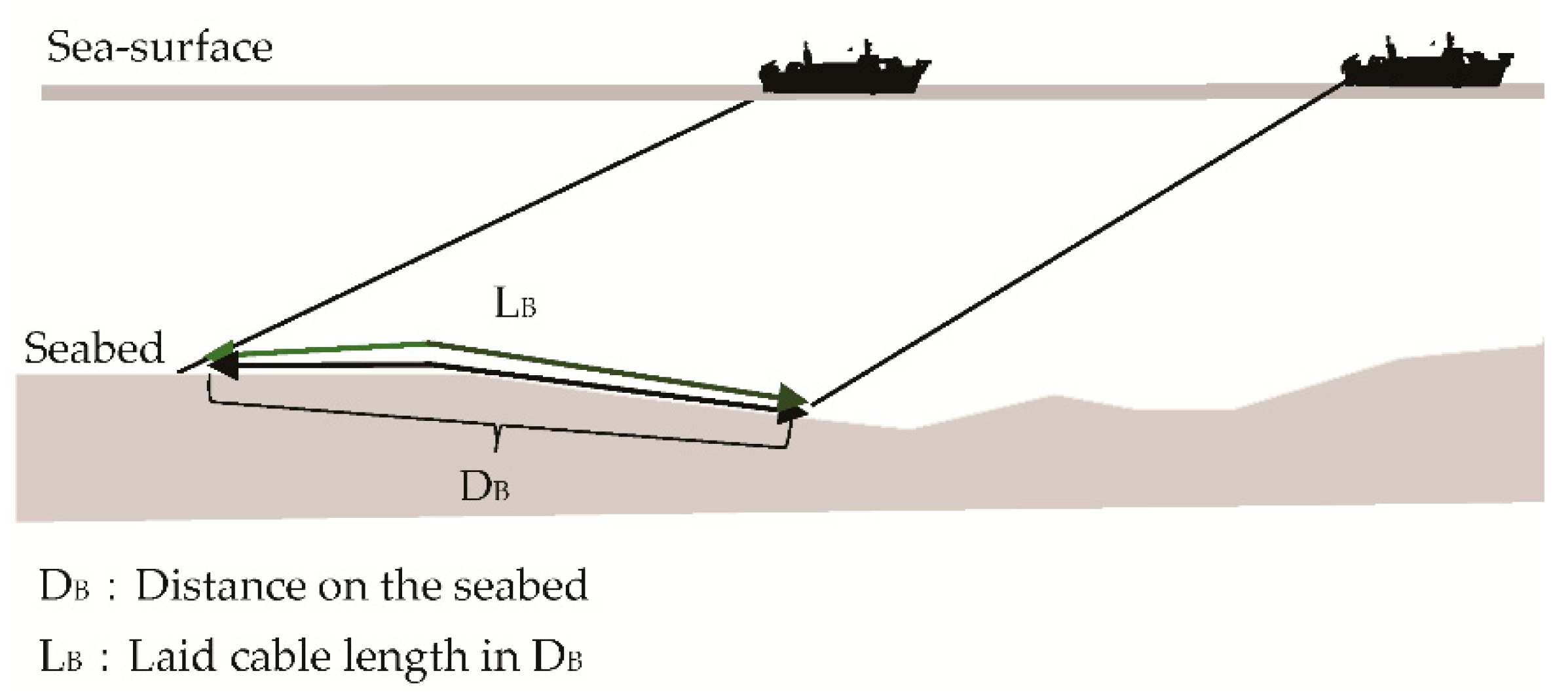
3.1. Definition of Slack

If the cable being laid is to follow the descending slope of the seabed, then it is necessary to lay the cable at a speed, V_C, that exceeds the laying ship speed, Vs. The percentage of this extra cable speed relative to the ship speed is called “slack.” The word “slack” is commonly used, without being precisely defined. There are several definitions, so it is necessary to clearly define these terms before continuing the discussion. The main definitions used here are:

(1)

Fill slack

The minimum required slack along changes in the slope of the seabed is defined as the fill slack. As an example, Figure 6 shows a cable being laid on the descending and ascending slopes of the seabed, and the fill slack is expressed in Equations (5) and (6).

Fill slack (descending slant) = (Vc − Vs)/Vs = (a + b − c)/c (%)

(5)

Fill slack (ascending slant) = (Vc − Vs) / Vs = (a – b − c)/c (%)

(6)

(2)

Seabed slack

The seabed slack is defined to accommodate the seabed profile. As an example, Figure 7 shows a conceptual diagram of seabed slack, which is defined by Equation (7).

Seabed slack = (L_B − D_B)/D_B (%)

(7)

The distance along the seabed, for this calculation, is interpolated from bathymetry information, obtained by the route survey before the system design.

(3)

Meaning of a Negative slack value

Assume that the ship is sailing at a constant speed and that there are no sea currents. If the cable pay-out rate is equal to the ship speed, then the cable tension at the ship will be nearly equal to the cable weight in the water, w·h [7]. Here, w is the cable weight per unit length in the water, and h is the water depth at which the cable reaches the seabed. Figure 8 shows the change in the cable catenary with negative slack. The seabed topography is flat, the distance moved by the ship from A to C in time t is Vst, and the cable laying length is denoted by Vct. When the cable laying length Vct is less than the distance moved by the ship Vst, the fill slack is defined by Equation (8).

Fill slack (Flat seabed) = (Vct − Vst)/Vst = Negative (%)

(8)

For positive slack, the tension at the point where the cable reaches the seabed is equal to zero, and for negative slack, extra cable tension T is generated and acts upon the cable. Thus, the practical cable tension at the ship Ts is expressed as (9):

Ts = w·h + T

(9)

While the ship sails from A to C (V_st), the shortage of the cable length can be approximated by the following Equation (10):

$$\overline{\mathrm{DE}}=\mathrm{X}-\mathrm{h}/\tan \mathsf{\alpha }$$

(10)

Negative slack means that the extra force, T, generated at the point of contact between the cable and the seabed causes drag on the cable. This can cause damage to the polyethylene sheath of the unarmored cable. The above situation also occurs on the seabed after laying the repeater and just before the repeater reaches the seabed. Section 3.4.2 presents the quantitative simulation of the area where negative slack occurs, due to the laying of repeaters.

3.2. Reason for Simulation

In conventional cable laying, engineers planned the ship speed and cable pay-out rate (based on their experience) and cable dynamics (based on a stationary response). In cable laying, the average fill slack greatly influences the cable characteristics. By measuring the average fill slack on the ship, the vessel and the cable engine are controlled to maintain the planned settings during the actual laying. However, since engineers only optimized the average fill slack on the ship because they could not measure the conditions of seabed cables, they could not know whether the cables were optimally laid.

To optimize cable laying, we must measure the seabed cable slack and tension in real time and feed this information back to the speed and course of the ship, as well as the rate of pay-out cables. Engineers can optimize the installation of the cable length on the seabed, based on the seabed slack calculated by the simulation of the system onboard. Compared to fill slack control, seabed slack control is an economically and mechanically superior control method that enables the laying of a cable system along undulations of the seabed, improving the construction quality.

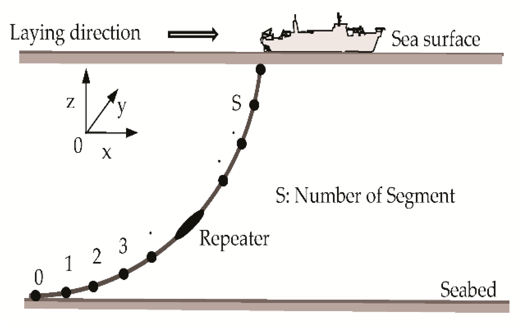
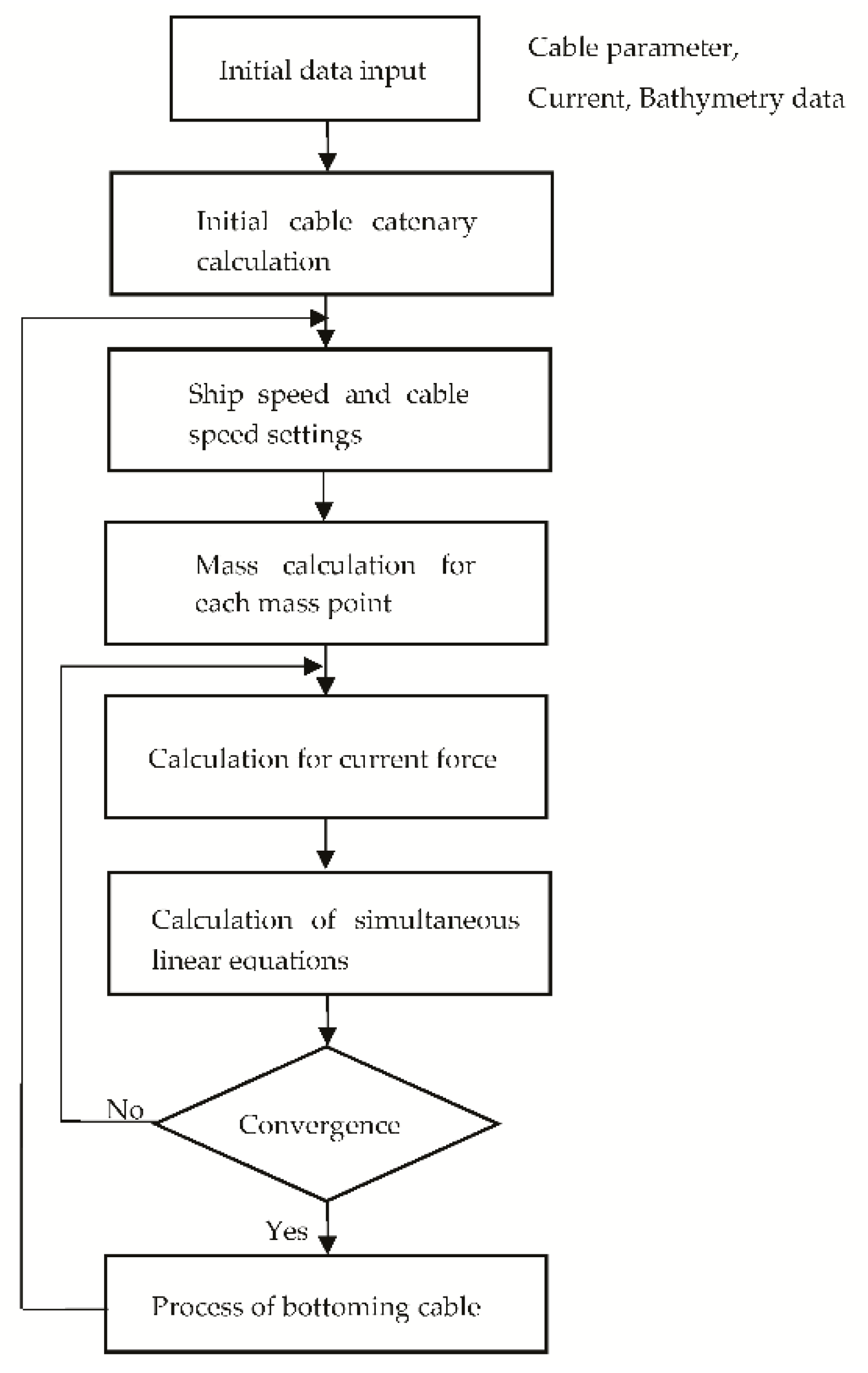
3.3. Calculation Procedure

At present, finite element procedures are very widely used in engineering analysis. Indeed, FEM (finite element method) is useful in virtually every field of engineering analysis. Traditional models of laying and recovering submarine cables deal with the behaviors of cables in a steady state. A 3D dynamic model using FEM has advantages over conventional models of cable laying and recovery. The cable catenary in the water is divided into multiple elements in this model, as shown in Figure 9. The mass and acting force of each element are considered to be concentrated at one point. Thus, the calculation proceeds in the actual program, according to the flowchart shown in Figure 10.

3.4. Simulation Analysis of Cable Behavior, including Repeaters

3.4.1. Typical Behavior of Cable Catenary in the Water

The upper figure in Figure 11 shows an example of the cable simulation from the sea surface to the seabed with one repeater. Black circles indicate the repeater, and solid lines indicate cables. After laying the repeater from the ship, the shape of the cable catenary, at both ends of the repeater, is gradually pulled locally toward the seabed by the weight of the repeater, and the change in catenary shape increases as the repeater descends. As a result, the repeater reaches the seabed faster than the cable at both ends. Hence, the cable drag area is behind the repeater (opposite the laying direction), due to negative slack and the increased cable tension on the seabed. Details are explained in the next section. The lower figure in Figure 11 shows the cable drag-start range from the repeater, based on the simulation results in Section 3.4.3.

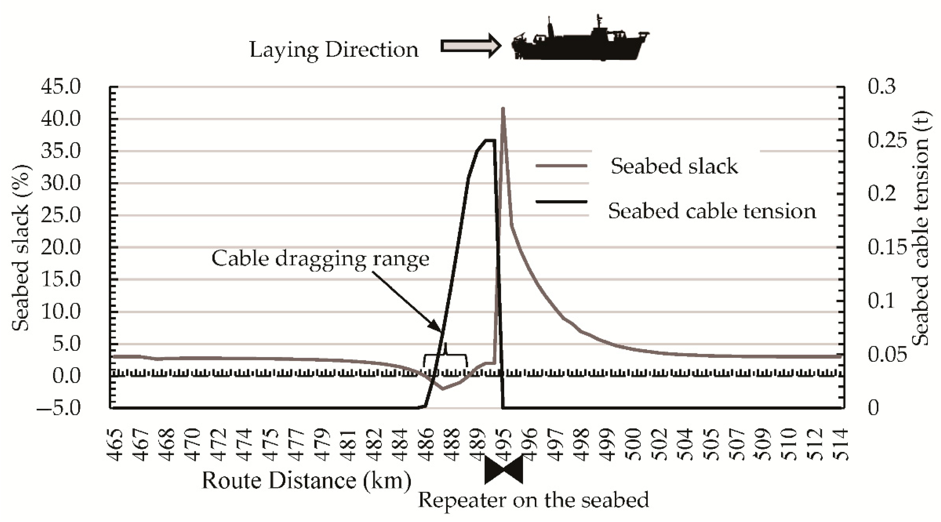
3.4.2. Simulation Analysis of Seabed Slack and Seabed Cable Tension, before and after the Repeater Reaches the Seabed

Figure 12 shows details of the simulated seabed slack and seabed cable tension changes before and after the repeater reaches the seabed under conditions of a fill slack of 3%, additional slack of 0%, laying speed of 7 km/h, water depth of 6000 m, flat seabed, and LW cable type.

The distance-based changes are as follows:

(1)

In the 465–484 km range, the seabed slack is 3%, which is the same as the fill slack, and the seabed tension is constant at 0 t.

(2)

At 484 km, the seabed slack begins to decrease.

(3)

In the 485–488.5 km range, the seabed slack decreases from zero to negative 2% and then gradually returns to zero. The increase in the seabed cable tension is inversely proportional to the change in the seabed slack, and when the seabed slack becomes positive, the seabed cable tension changes at a slower rate. As a result, the cable behind the repeater will be dragged by the increased seabed cable tension, due to negative slack.

(4)

At 489 km, the seabed slack increases to positive 2%, and the curve of the seabed cable tension change becomes flat. As a result, the drag force acting on the cable will be gradually reduced.

(5)

At 495 km, the repeater reaches the seabed, and the seabed cable tension suddenly drops from about 0.27 t to zero. The seabed slack rises sharply to about 43% and then slowly declines. The seabed slack rises rapidly because the cable is pulled while it sinks, due to the weight of the repeater; for that reason, when the repeater reaches the seabed, the cable length is longer than the distance on the seabed.

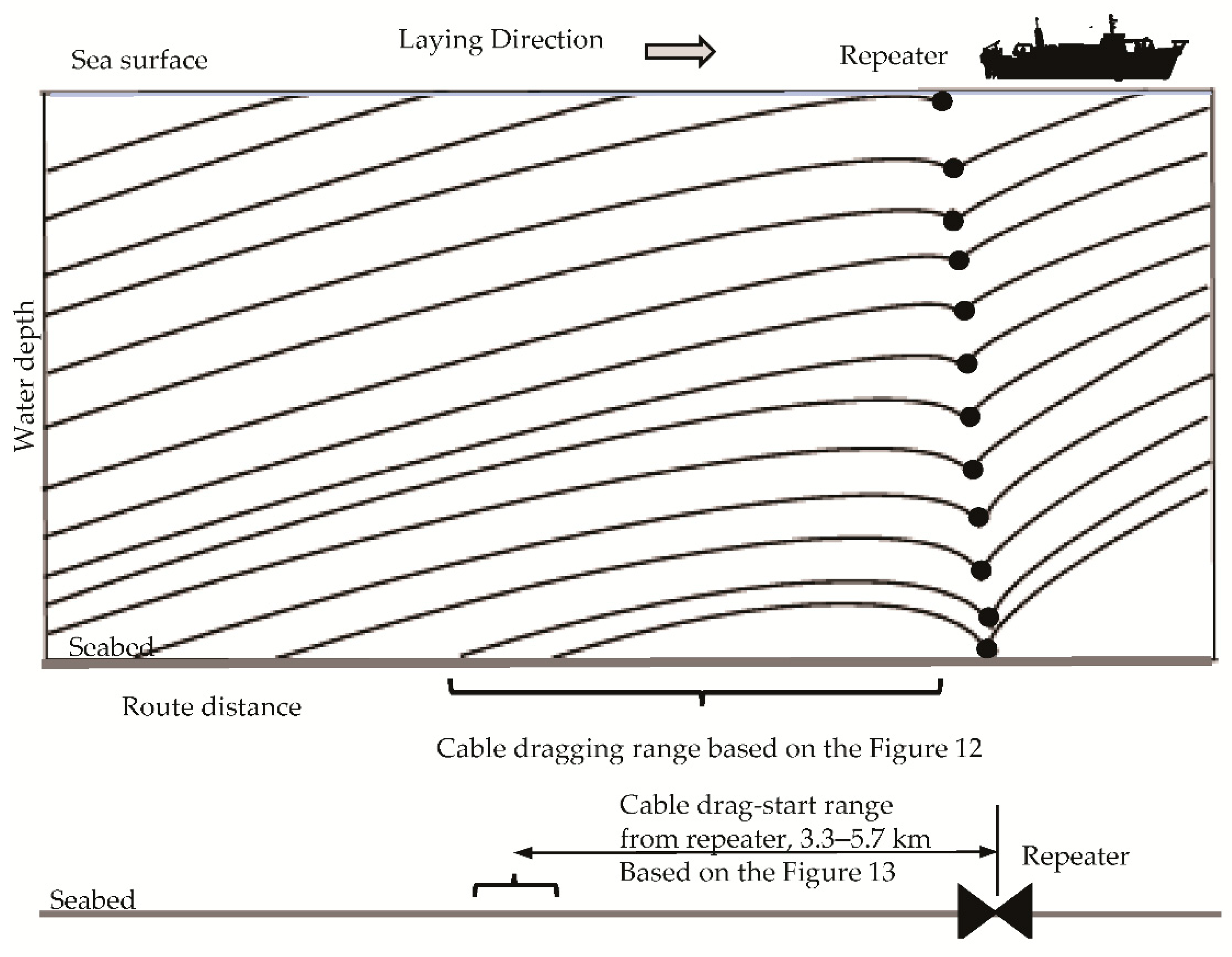
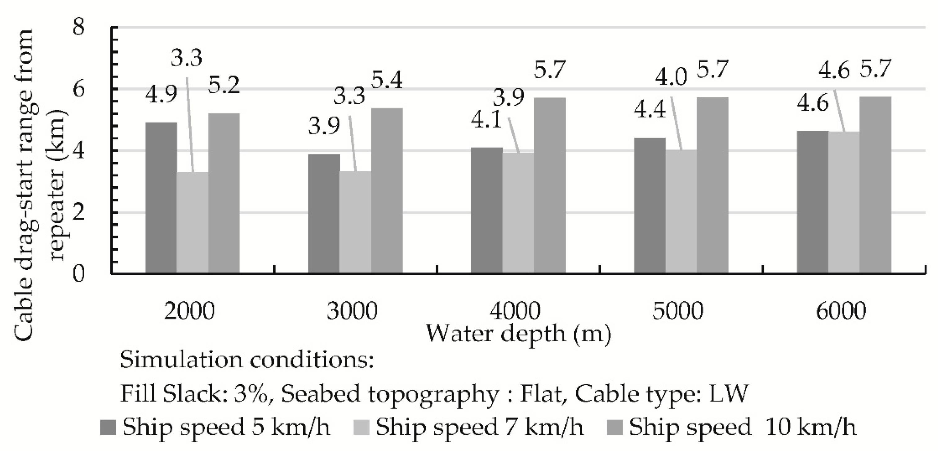
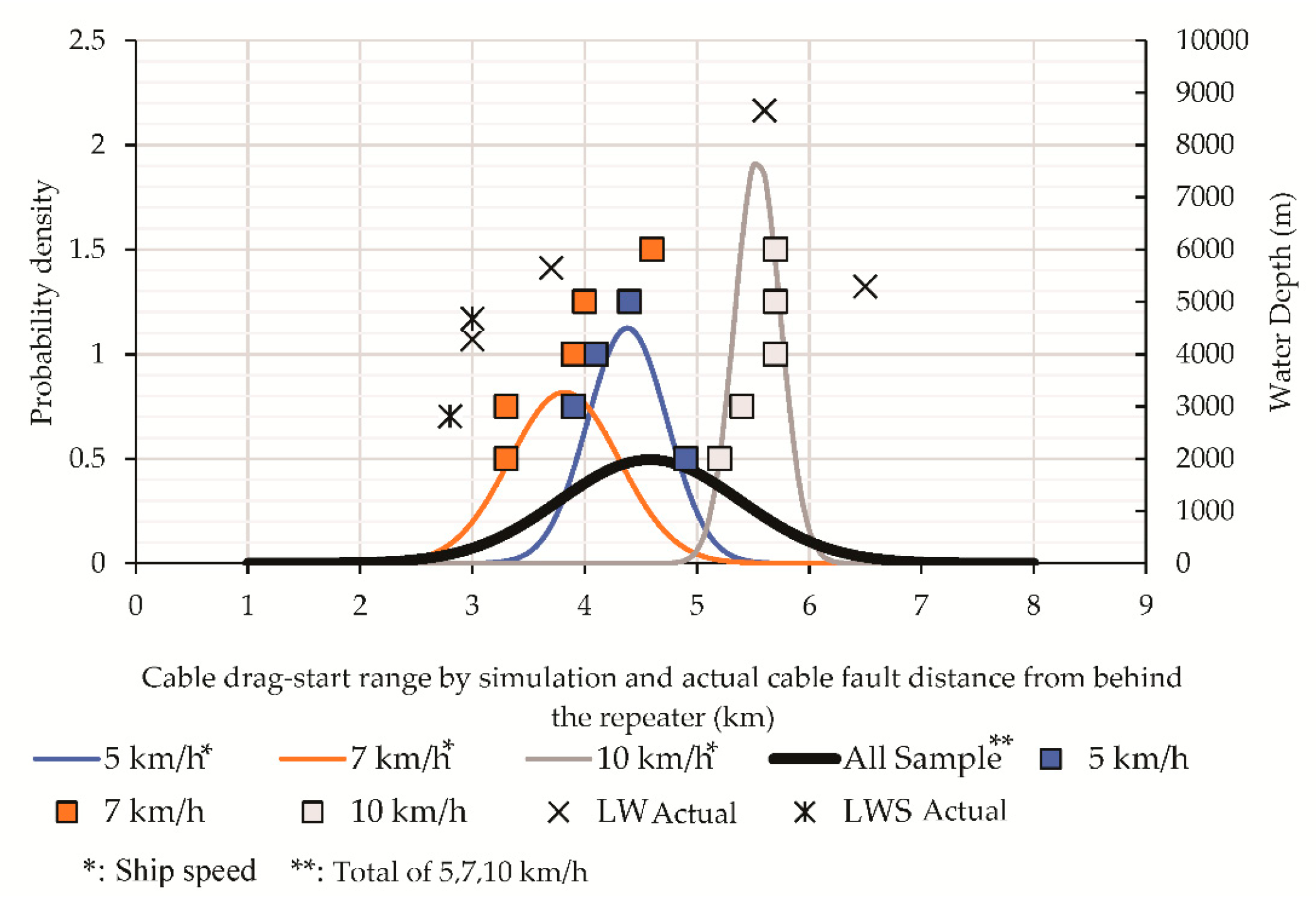
3.4.3. Analysis of Cable Drag-Start Range from Repeater

Figure 13 shows the change in the cable drag-start range from the repeater when the repeater is laid at depths of 2000–6000 m, with laying speeds of 5–10 km/h. The cable drag-start distance from the repeater is defined by the location where the seabed slack changes to 0%. The simulation results show that the cable drag-start range from the repeater is distributed from 3.3 to 5.7 km. It does not have a strong relationship with ship speed and water depth. This simulation result suggests that the cable catenary shape near the seabed at great water depths becomes almost horizontal and is, therefore, not strongly dependent on the laying speed within a range of 5–10 km/h.

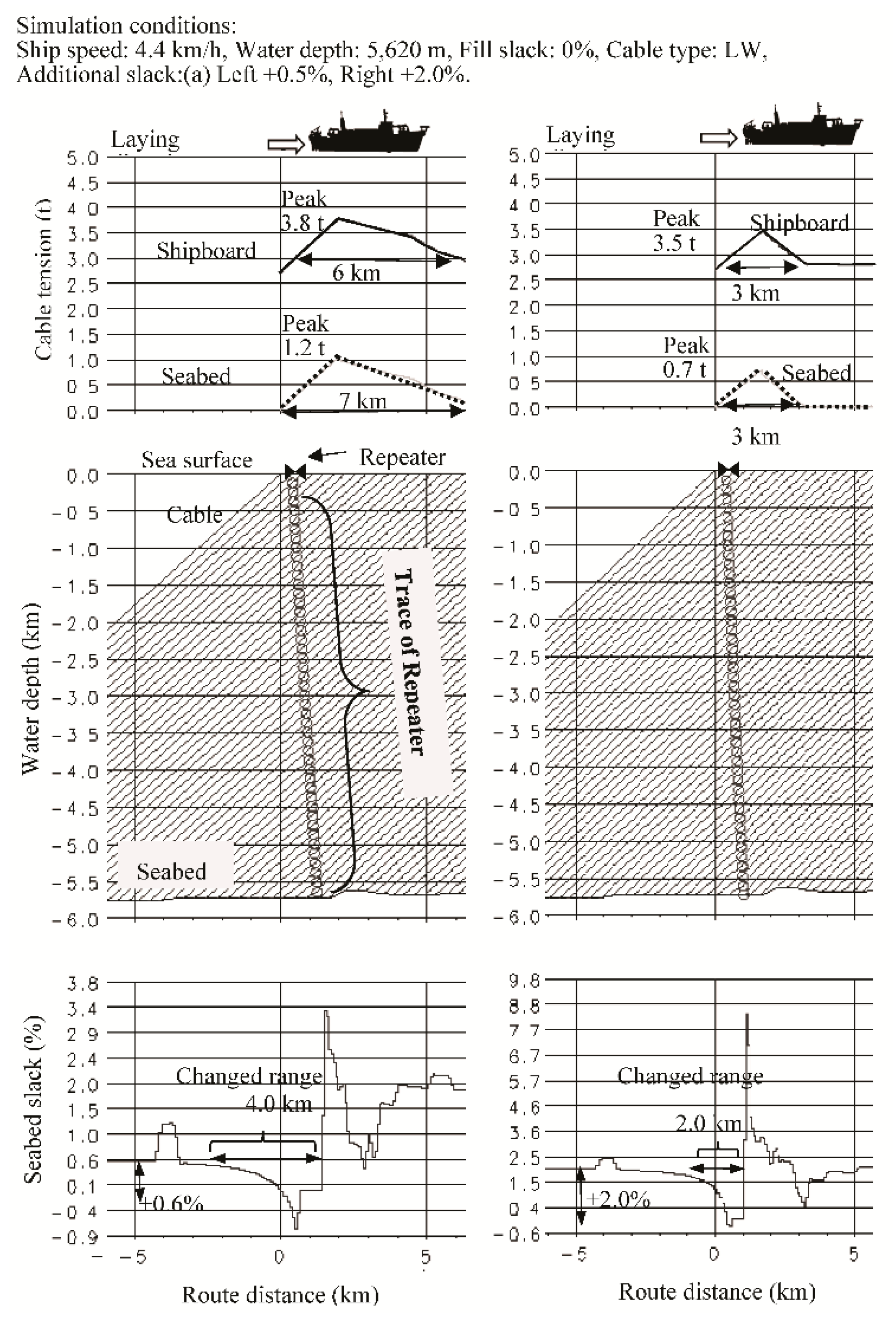
3.5. Comparative Verification of Cable Behavior in Different Repeater Laying Conditions

From the simulation results in Section 3.4.2, when the seabed slack decreases and the seabed cable tension increases in the range just before the repeater reaches the seabed, the cable will drag. The reduction in the drag force on the cable is achieved by shortening the distance over which the seabed cable tension changes at the point where the cable reaches the seabed and by decreasing its peak value just before the repeater reaches the seabed. Therefore, the mechanical reliability of the cable is expected to improve. Figure 14 shows two simulation cases with different additional slack, including the repeater. The upper figure shows the cable tension on the ship (straight line) and seabed (dashed line); the middle figure shows the path traced by a descending repeater (circle). The lower figure shows the continuous change in the seabed slack.

Compared to the additional slack of +0.5%, +2.0% reduces the peak and the range of the cable tension change on both the ship and the seabed, showing a 50% reduction in seabed slack and a change in the range from 4.0 km to 2.0 km. This result confirms that increasing the additional slack is an effective method of reducing the cable drag range on the seabed when laying a repeater. As an economical and effective method, it is practical to set the additional slack only in the actual fault range behind the repeater. Details are described in Section 5.

4. Study of Cable Faults Triggered by Laying Repeater at Great Water Depths

For the analysis in this section, we collected data on actual cable faults triggered by laying repeaters at great water depths, in order to compare and verify factors contributing to cable damage, based on the simulation analysis in Section 3. In addition, since the damage to unarmored cables was closely related to the surface conditions of the seafloor, we examined the literature on seafloor seismographs and physical evidence obtained from cable maintenance activities to understand the characteristics of the deep seafloor.

4.1. Collection and Classification of Cable Faults behind the Repeater

We reviewed the system maintenance records of cable faults at water depths greater than 1500 m, where human activity is not involved in the Northwest Pacific. The fault results were grouped under the following titles:

(1)

period: years 1999–2016;

(2)

time and date of the occurrence of a fault;

(3)

laying direction of the system in the installation stage;

(4)

fault category;

(5)

cable types;

(6)

water depth;

(7)

cable fault within 7 km behind the repeater, determined by the maximum cable drag-start distance from the repeater (5.7 km) in the simulation in Section 3.4.3 and an uncertainty factor of about 1.2 times;

(8)

the topographic gradient of the seabed was obtained by calculations, based on the distance between two points, changes in the water depth, and the water depth at the fault point;

(9)

time from system deployment to the occurrence of a fault.

Out of 21 total faults, 6 cable faults (within 7 km behind the repeater) were due to repeater laying, while cable faults caused by the 2011 Tohoku Earthquake (off the Pacific coast) were not included. The maintenance records cover many decommissioned and in-service cable systems. Typically, a system failure is reported for a specific cable system, based on the time of occurrence, fault location, water depth, fault type, seabed gradient, and other relevant environmental factors. Therefore, the maintenance record is a primary document that allows us to compile cable faults related to repeater laying. The recorded positions in the maintenance records are reliable because the vessels used for maintenance are equipped with DGPS (differential global positioning system), which provides high-accuracy positioning, with an error of less than 1 m for the vessel on the sea surface, from which accurate fault positions can be determined.

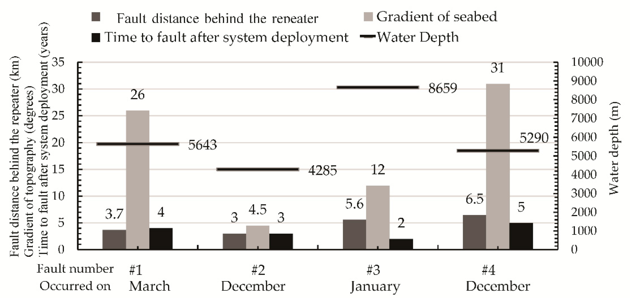
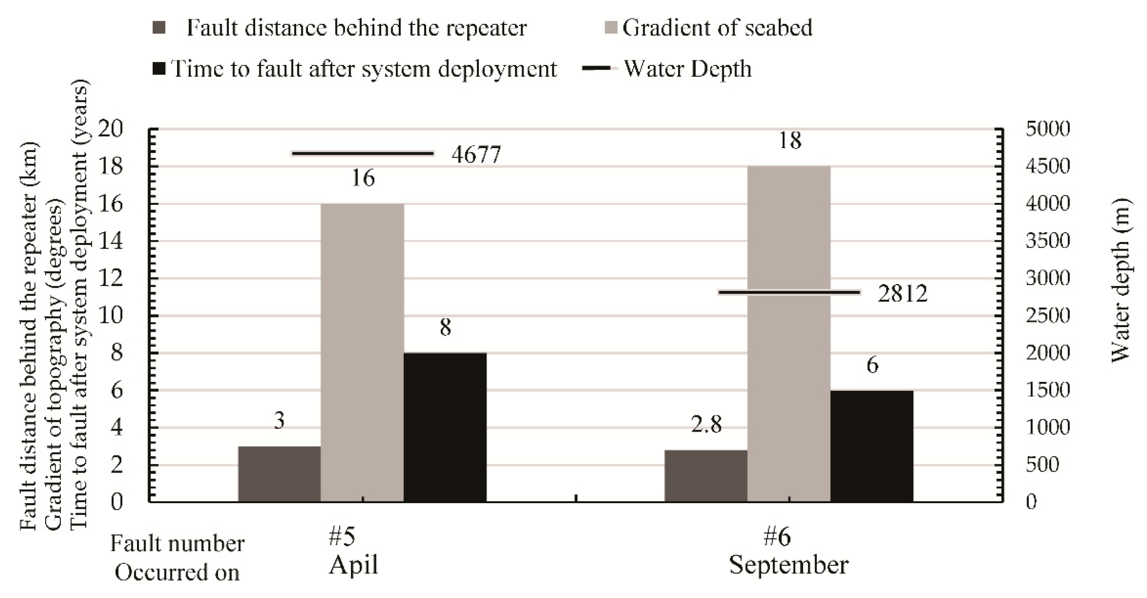
4.2. Results of Cable Fault Analysis

(1)

Fault category: all shunt (insulation fault) for LW and LWS types.

(2)

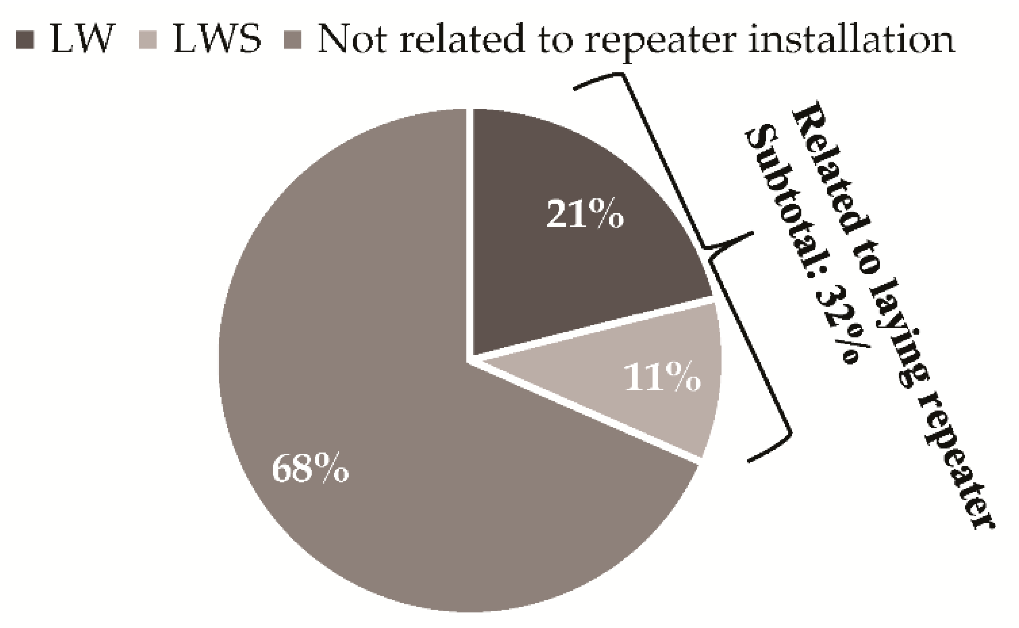
The proportion and distribution of cable faults.

Figure 15 shows the proportion of LW and LWS cable faults triggered by laying repeaters relative to all cable faults, and Figure 16 shows the fault location for each cable type.

(3)

Details of the fault.

Figure 17 and Figure 18 show the individual fault situations for LW and LWS cables, namely, the fault distance in the cable drag range behind the repeater, the gradient of the seabed, the time to the fault after system deployment, and the water depth.

In Figure 19, the normal distribution of the cable drag-start range behind the repeater in various laying conditions, based on the simulation results in Section 3.4.3 (see Figure 13) is compared with the actual cable fault distance.

4.3. Summary of the Fault Analysis in the Northwest Pacific

The above fault analysis reveals an approximate trend with the following characteristics.

(1)

Overall trend.

A total of 32% of all faults are related to laying repeaters, with 21% for LW and 11% for LWS (see Figure 15). Faults occur nearly twice as often for LW as LWS.

(2)

Geographical distribution of fault locations.

The locations of cable faults tend to be distributed along trenches and seamounts. This is the case for faults #2, #5, and #6, which occurred along the Emperor Seamounts (see Figure 16).

(3)

Fault distance behind the repeater.

The actual fault distance behind the repeater is 3.0–6.5 km for LW and 2.8–3.0 km for LWS, and the laying ship speed for each data point is unknown. The cable drag-start range behind the repeater is 3.3–5.7 km in various laying conditions (laying ship speed and water depth) in the simulation (see Figure 13). These values mean that the simulation result matches well with the actual cable fault range (see Figure 19).

(4)

Topographic gradient of the seabed.

The seabed topography is likely to cause a cable fault when the gradient is 12 degrees or more for LW cables and 16 degrees or more for LWS (see Figure 17 and Figure 18). Based on these findings, unarmored cable faults are more likely to occur if the seabed gradient exceeds 12 degrees. However, LW fault #2 was observed in a low-gradient region of 4.5 degrees.

(5)

Time to fault after system deployment and total fault number.

In LW cables, faults tend to occur within the first five years after deployment. LWS cable faults tend to appear from six to eight years after deployment. The reason is that the LWS cable is mechanically more robust than the LW cable (see Figure 3).

(6)

Season of fault occurrence.

In the Emperor Seamount area, both LW and LWS cable faults occur from autumn to spring, as observed for faults #2, #5, and #6.

(7)

Fault-free area.

A fault-free area can be observed within 2.8 km behind the repeater for both the LW and LWS cable types. This observation is supported by the simulation results in Section 3.4.2 (4).

4.4. Consideration of Geographical Locations Where Cable Faults Tend to Occur

In this section, we consider the causes of cable faults that tend to be distributed in trenches and Emperor Seamount areas, which is described in Section 4.3. The factors are verified based on the cabled submarine seismic observation system in the trench around Japan and system maintenance records.

4.4.1. Cable Faults in Trenches

In order to verify the causes of faults, we reviewed the literature on the cabled seismic observation system near the trench east of Japan and the maintenance records of the fiber-optic submarine cable system.

(1)

Review of the literature on cabled submarine seismic observation system

Several optical-cabled, ocean-bottom observation systems have been installed in trenches on the Pacific side of Japan. They function as disaster prevention infrastructure, in preparation for natural disasters. It was found that the roll angle of seismometers had measured ground shaking associated with the earthquake, rather than the pitch angle owing to the cylindrical shape of the pressure vessel in the unburied section. This cause indicates that the pressure vessels themselves can tumble or be rotated by strong motions because of unsatisfactory coupling between the pressure vessel and the hard seabed rock, and the flat area is limited, due to the rough undulations of the seabed [17,18]. This fact suggests that the seabed surface of the trench is rough and hard underneath.

(2)

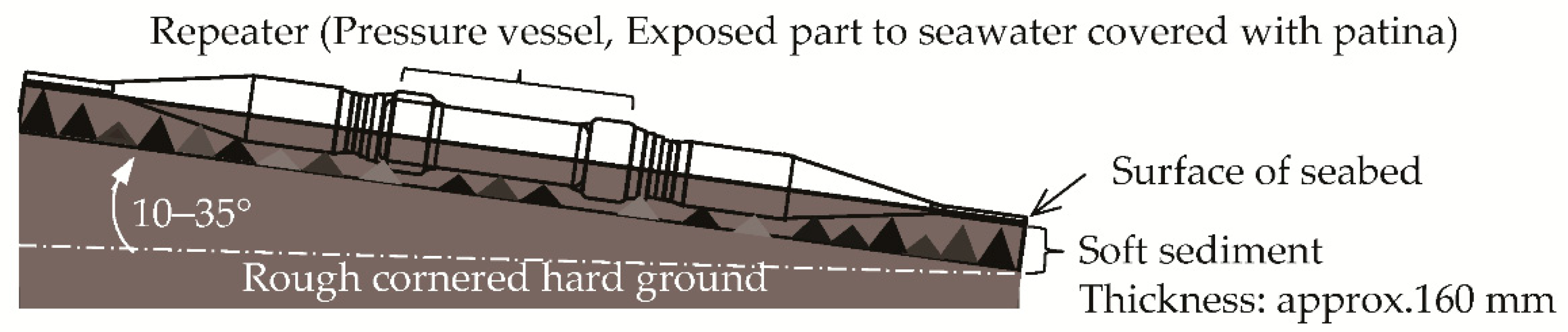
Features of the deep seafloor surface, based on physical evidence of submarine cable system.

Figure 20 shows the positions of recovered repeaters in the Northwest Pacific basin on a flat seabed at depths of 5400–5500 m and the Nankai trough on a sloping seabed at a depth of 3300 m, based on submarine cable maintenance records. All three recovered repeaters show similar changes on the surface of the pressure vessel, with Figure 21 showing the appearance of repeater C.

4.4.2. A Factor of Unarmored Cable Damage by the Deep Seafloor

From the above results, the following can be inferred. The polyethylene sheath of unarmored cables is mechanically vulnerable to hard, deep seafloor surfaces with rough corners in negative slack areas. Figure 22 shows an example of a repeater laid on the seabed of a subduction zone or the Emperor Seamounts.

5. Discussion on the Mitigation of Cable Faults Associated with Laying Repeater

5.1. Best Approach to Protecting Submarine Cable Systems from Natural Hazards

The Northwest Pacific region is tectonically active, and as a result of the movement of the continental plates, large-scale trenches and chains of seamounts have formed along its boundaries. Moreover, the combination of frequent earthquakes, faulting, landslides, and turbidity currents has produced steep slopes or steps and caused seriously eroded and irregular seabed topography [5]. It is clear that submarine cable systems, especially unarmored cables in the deep sea, are exposed to potential threats from natural hazards in the above areas. It is recommended that cable routes avoid the above areas in the canyon profile. In the intervening reaches of the canyon, there is less erosion, so the cables have a better chance of survival (see Section 5.3, Table 4, step 3).

5.2. Shipboard Cable Tension Measurement When Repeater Reaches the Seabed

Based on the simulation results in Section 3.5, we verified the effect of different additional slack and laying cable speeds during the laying operation to reduce the drag range of the cable behind the repeater.

Table 3. Repeater laying conditions for Figure 23a–c.

Items/Figure 23	a	b	c
Ship speed (km/h)	6.0	10.0	1.3
Water depth (m)	5400	5423	2620
Fill slack (%)	0.0	0.0	−1.7
Additional slack (%)	+1.6	+2.5	0.0
Cable type	LW	LW	LWS

shows repeater laying conditions for Figure 23a–c, and the same Figure shows the changes in the shipboard cable tension, measured by a calibrated load cell when the repeater reached the seabed. In each case, when the repeater reached the seabed, the cable tension on the ship exceeded the planned cable tension (w·h), indicating that negative slack caused extra tension at the contact point between the cable and the seabed. Since the cable tension cannot be measured directly (at the point where the cable reaches the seabed), it can be indirectly determined, based on the change in the shipboard cable tension using Equation (9) in Section 3.1 (3).

Comparing Figure 23a,b, it can be seen in Figure 23b that the ranges of changes in the shipboard cable tension (from 8 to 4 kN) and its distance (from 5 to 2.4 km) are each reduced by approximately 50% of additional slack. Comparing Figure 23a,c, it is found in Figure 23c that the range of change in shipboard cable tension decreases (from 8 to 5 kN) by 38% by a slower laying speed. A reduction in the shipboard cable tension (when the repeater reaches the seabed), due to the additional slack and slower laying speed, suggests that the cable drag range is shortened, and its force is reduced, based on the simulation results in Section 3.4.2.

5.3. Proposal to Minimize the Impact of Cable Faults Relating to Laying Repeaters

We explored multiple measures, including a practical solution, such as changing the planned cable route or cable type, to mitigate cable faults. However, ultimately, we decided that the best path forward was to focus on cost-effectiveness. In order to optimize these measures, we investigated the construction process of the submarine cable system. A typical scenario is usually divided into the following steps [19]. The repeater span is determined during the design step of optical signal performance in Step 3 [20].

• Step 1: marine route survey;
• Step 2: route design;
• Step 3: submarine plant design;
• Step 4: submergible equipment manufacturing;
• Step 5: system assembly and test;
• Step 6: marine installation, including laying design;
• Step 7: land cable and terminal equipment manufacturing, installation, and test;
• Step 8: system test.

Comparative Verification of Each Process to Reduce Cable Faults

Steps 2 and 3, above, fundamentally eliminate the risk of cable damage associated with laying a repeater by changing to a route with a lower risk of cable damage or applying mechanically reinforced cables. Step 6, on the other hand, is a measure that mitigates cable damage by allocating more cables to specific risk areas associated with laying repeaters.

Table 4. Comparison of measures and cost impact on construction costs.

Steps	Measures		Cost Impact
Step 3	If the planned repeater location on the seabed cannot avoid the hazardous terrain, place the repeater outside the range.		High
	If the planned repeater location on the seabed cannot avoid the hazardous terrain, use the LWS cable within the allowable water depth range.		Middle
Step 6	Method 1	Apply “a” or “b” at cable lengths to repeaters 2.8-6.5 km after laying the repeater, not applied.	Low
		a. Compensate for +3.0 to +4.5% extra cable slack
		b. Decrease the laying speed by half with transient cable slack
	Method 2	Keep laying cable at a low speed less than 2 km/h

shows our proposed, specific measures with a comparative evaluation of their economic impact on construction costs. Here, the tendency for a cable fault to be caused by laying a repeater is defined as the presence of hazardous terrain, due to a topographic gradient larger than 12 degrees, within 6.5 km behind the repeater on the seabed. This definition is based on the experiments, simulations, and discussions presented in the above sections.

Evaluation of Table 4:

The measures in Step 3, which fundamentally solve the cable fault triggered by laying repeaters, are economically disadvantageous.

Fundamental measures: Step 3

This step directly leads to an increase in capital expenditure because the scale of the system modification is large.

On the other hand, the measures in Step 6, to mitigate the same fault, are practical because they are cost-effective, based on the following.

Mitigation measures: Step 6

Adopting Step 6 is realistic and economically advantageous.

Method 1: compensate slack in a limited range that drags the cable behind the repeater on the seabed:

• a: increase the extra slack to +3–4.5% [5], which requires a cable length of about 150 m;
• b: reduce the laying speed by half.

For example, if the laying speed is reduced from 7.0 to 3.5 km/h, it needs an additional 160 m of cable length as transient slack.

These methods do not affect the performance of the laying operation because the laying speed can be maintained in the high-speed range of 5–10 km/h, which is economically advantageous for system construction work of long-haul projects, such as transpacific lines.

Method 2: When laying a repeater, keep the cable catenary length short in the water by slowing the laying speed. This is valid for a location where the seabed topography is severe, such as trenches and seamount terrains, or where repair work is occurring in a limited area.

6. Conclusions

In this study, analysis and comparative evaluation based on experiments, simulations, and submarine cable maintenance records quantitatively demonstrated the cable fault mechanism and actual faults associated with laying repeaters. The simulations revealed the potential risk range of cable faults behind repeaters, and the results are in close agreement with the actual fault situation. Regarding the seafloor surface in the deep sea, based on the observation results of the seafloor seismometer and the physical evidence of the pressure vessel of the recovered repeater, we also established that cable faults tend to be distributed in trenches and seamount areas. Based on a discussion of mitigation measures for cable faults associated with laying repeaters, some cost-effective approaches are proposed. These proposals have important significance in an information-oriented society, where digitalization is advanced by improving the construction quality of systems and realizing mechanically stable systems.

References

- Ash, S.; Godwin, M.; Green, M.; Morgan, N. From Elektron to “e” Commerce: 150 Years of Laying Submarine Cables; Global Marine Systems: Chelmsford, UK, 2000; pp. 13, 17, 51. ISBN 0953907805. [Google Scholar]
- Wildman Whitehouse Patent 2027 of 1860, Specification in Pursuance of the Conditions of the Letters Patent, Filed by the said Edward Orange Wildman Whitehouse in the Great Seal Patent Office on the 23 February 1861. Available online: https://atlantic-cable.com/Books/Whitehouse/Patents/2027.htm (accessed on 30 June 2020).
- NEC Press Release; June 2016. Faster Cable System Is Ready for Service, Boosts Trans-Pacific Capacity, and Connectivity. Available online: https://www.nec.com/en/press/201606/global_20160629_02.html (accessed on 30 July 2021).
- Gavey, R.; Carter, L.; Liu, J.T.; Talling, P.J.; Hsu, R.; Pope, E.; Evans, G. Frequent Sediment Density Flows from 2006 to 2015, Triggered by Competing Seismic and Weather Events: Observations from subsea Cable Breaks Off Southern Taiwan. Mar. Geol. 2017, 384, 147–158. [Google Scholar] [CrossRef]
- Ogasawara, Y.; Natsu, W. Proposal for reducing the failure rate of fiber-optic submarine cables in deep-sea based on fault analysis and experiments. J. Adv. Mar. Sci. Technol. Soc. 2020, 25, 1–12. [Google Scholar] [CrossRef]
- Burnett, R.; Beckman, R.C.; Davenport, T.M. Submarine Cables: The Handbook of Low and Policy; Martinus Nijhoff Publishers: Boston, MA, USA, 2014; p. 31. ISBN 978-90-04-26033-7. [Google Scholar]
- Zajac, E.E. Dynamics and kinematics of the laying and recovery of submarine cable. Bell Syst. Tech. J. 1957, 36, 1129–1207. [Google Scholar] [CrossRef]
- Kishimoto, R.; Kitazawa, I. Dynamic Behavior of a Submarine Cable in a Uniform Sea Flow. Bull. JSME 1982, 25, 204–212. [Google Scholar] [CrossRef]
- Kojima, J. Three-Dimensional Dynamic Analysis for Laying and Recovery of Optical Submarine Cables. J. Soc. Nav. Archit. Jpn. 1990, 1990, 309–318. (In Japanese) [Google Scholar] [CrossRef]
- Niiro, Y.; Ejiri, Y.; Yamamoto, H. The first Transpacific optical fiber submarine cable system. In Proceedings of the IEEE International Conference on Communications, World Prosperity Through Communications, Boston, MA, USA, 11–14 June 1989; pp. 1520–1524. [Google Scholar] [CrossRef]
- Maurice, E.K.; Ron, J.R.; Robert, K.S.; Sheridan, S.; Irish, O.B.; Wall, D.; Waterworth, G.; Perratt, B.; Wilson, S.; Holden, S. Global Trends in Submarine Cable System Faults 2019 UPDATE. Presented at Oral Session OP 8-1, Suboptic 2019 New Orleans, USA. 2019. Available online: https://suboptic2019.com/suboptic-2019-papers-archive/ (accessed on 25 June 2020).
- Matthew, P. Wood and Lionel Carter. Whale Entanglements with Submarine Telecommunication Cables. IEEE J. Ocean. Eng. Soc. 2008, 33, 445–450. [Google Scholar] [CrossRef]
- Norimatsu, N.; Marugome, I.; Noguchi, Y.; Yamazaki, Y.; Yamamoto, H. Design and Test result of os-560M optical submarine cable, repeater housing, and coupling. ITE ITEJ Tech. Rep. 1991, 17, 17–23. ISSN 0386-4227(In Japanese) [Google Scholar] [CrossRef]
- Davis, J.R. Copper and Copper Alloys, ASM International c2001 ASM Specialty Handbook; Prepared under the Direction of the ASM International Handbook Committee: Materials Park, OH, USA, 2001; ISBN 9780871707268. [Google Scholar]
- Nishida, T.; Nagatomi, O. Latest Technologies and the OCC-SC300 Optical Submarine Cable. NEC Tech. J. 2010, 5, 18–22. [Google Scholar]
- Akiba, S.; Nishi, S. Submarine Cable Network Systems; NTT Quality Printing Service Co.: Tokyo, Japan, 2001; pp. 15–17, 262–264. [Google Scholar]
- Takagi, R.; Uchida, N.; Nakayama, T.; Azuma, R.; Ishigami, A.; Okada, T.; Nakamura, T.; Shiomi, K. Estimation of the Orientations of the S-net Cabled Ocean-Bottom Sensors. Seismol. Res. Lett. 2019, 90, 2175–2187. [Google Scholar] [CrossRef]
- Nakamura, T.; Hashimoto, N. Rotation motions of cabled ocean-bottom seismic stations during the 2011 Tohoku earthquake and their effects on magnitude estimation for early warnings. Geophys. J. Int. 2019, 216, 1413–1427. [Google Scholar] [CrossRef] [Green Version]
- Ohta, T.; Nishiyama, T. Route Design/Cable Laying Technologies for Optical Submarine Cables. NEC Tech. J. 2010, 5, 46–50. [Google Scholar]
- Yoneyama, K.; Sakuyama, H.; Hagisawa, A. Construction Technology for Use in Repeated Transoceanic Optical Submarine Cable Systems. NEC Tech. J. 2010, 5, 41–45. [Google Scholar]