
Method for the Coordination of Referencing of Autonomous Underwater Vehicles to Man-Made Objects Using Stereo Images


Abstract
:1. Introduction
Problem Statement
2. Method for Coordinate Referencing
2.1. SPS Model
2.2. Identification of the SPS Feature Points
- FPs matching on images of two stereo pairs;
- Calculation of 3D coordinates of the corresponding points in ;
- Computation of the local matrix to transform the coordinates at the current stage;
- Computation of matrix via combining local matrices from the previous stages;
- Calculation of absolute coordinates, sequentially applying two transformations—.
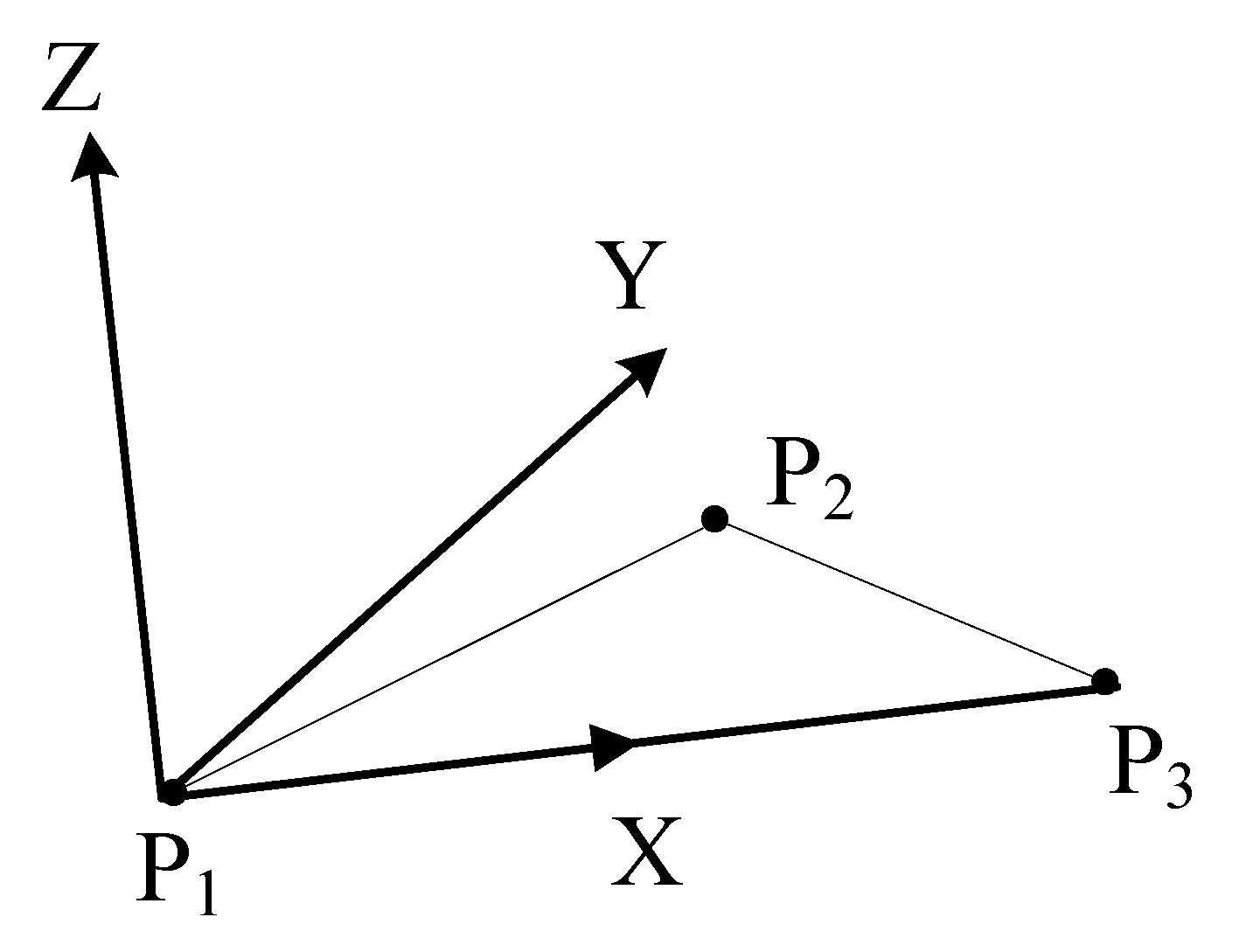
2.2.1. Stage 1
2.2.2. Stage 2
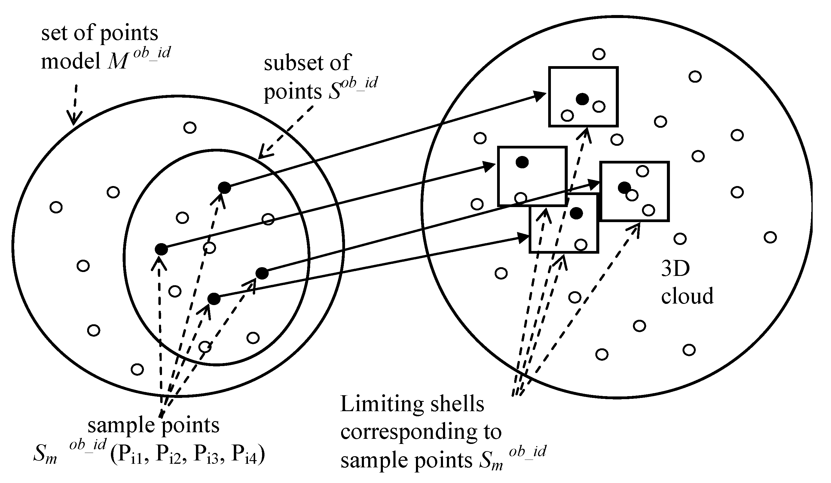
- On set of the points of the object model (see stage 1), a set of samples is generated, where m—the sample number, q—the sample length. The number of possible samples is defined by the number of permutations of n − q at a given time—;
- The set of distances is constructed, where is the distance between points and . Here, and are the numbers of points in the object model , and indices k and s are related to the numbering of points in sample , which is linked to each sample . There are elements in set ;
- The set of samples , comprised of the 3D cloud points, is generated for each sample of the object model. Here, n is the number of samples. The point from list , connected to point (see stage 1), is taken as the element of sample . The number of the generated samples is defined by the number of lists q and the lengths of these lists. For example, if q = 3, and the lengths of the corresponding lists are length1, length2, length3, the number of samples will be length1⋅ length2 ⋅ length3;
- The set of distances is constructed, where is the distance between points and —here, indices k and s are related to the numbering of points in the sample, and is linked to each sample . There are elements in set ;
- For a sample (step 1) from the object model, the sample (par.3) from the 3D cloud is sought, such that . Here, the equivalence means the equivalence between all the corresponding pairs of elements: . The error ∆ is determined by the accuracy of measuring the coordinates of the 3D cloud points (depending on the resolution of pictures and the distance between the camera and the points). In that case, with consideration for the above-described rules of forming samples, the determined correspondence between sample and sample enables the unambiguous identification of the points of the 3D cloud that belong to the SPS object, and for them to be matched with the object model points;
- If there are no corresponding points found in the 3D cloud for the specified length q of sample , the correspondence for a smaller sample shall be searched for, i.e., for . It should be noted that the implementation of searching, aimed at detecting the maximum number of points matched to the SPS object model’s points, in the 3D cloud increases the degree of certainty of object identification. Subsequent to the identification of several points (three as a minimum) belonging to the SPS object, in the 3D cloud, the coordinate referencing of the AUV to the SPS can be performed. Using more FPs would improve the accuracy of the method.
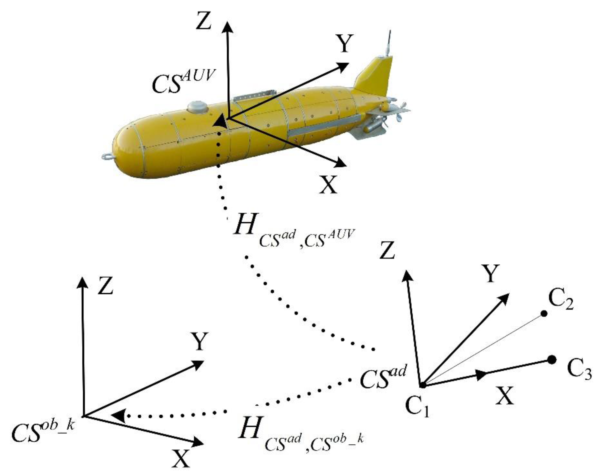
2.3. Calculation of the Matrix of the Geometric Transformation of the Points from the AUV CS to the SPS Object CS
Other Methods for Calculating the Transformation from the AUV CS to the CS of the SPS Object
2.4. Calculation of the AUV Coordinates in the SPS CS
3. Experiments
3.1. Experiments with a Virtual Scene
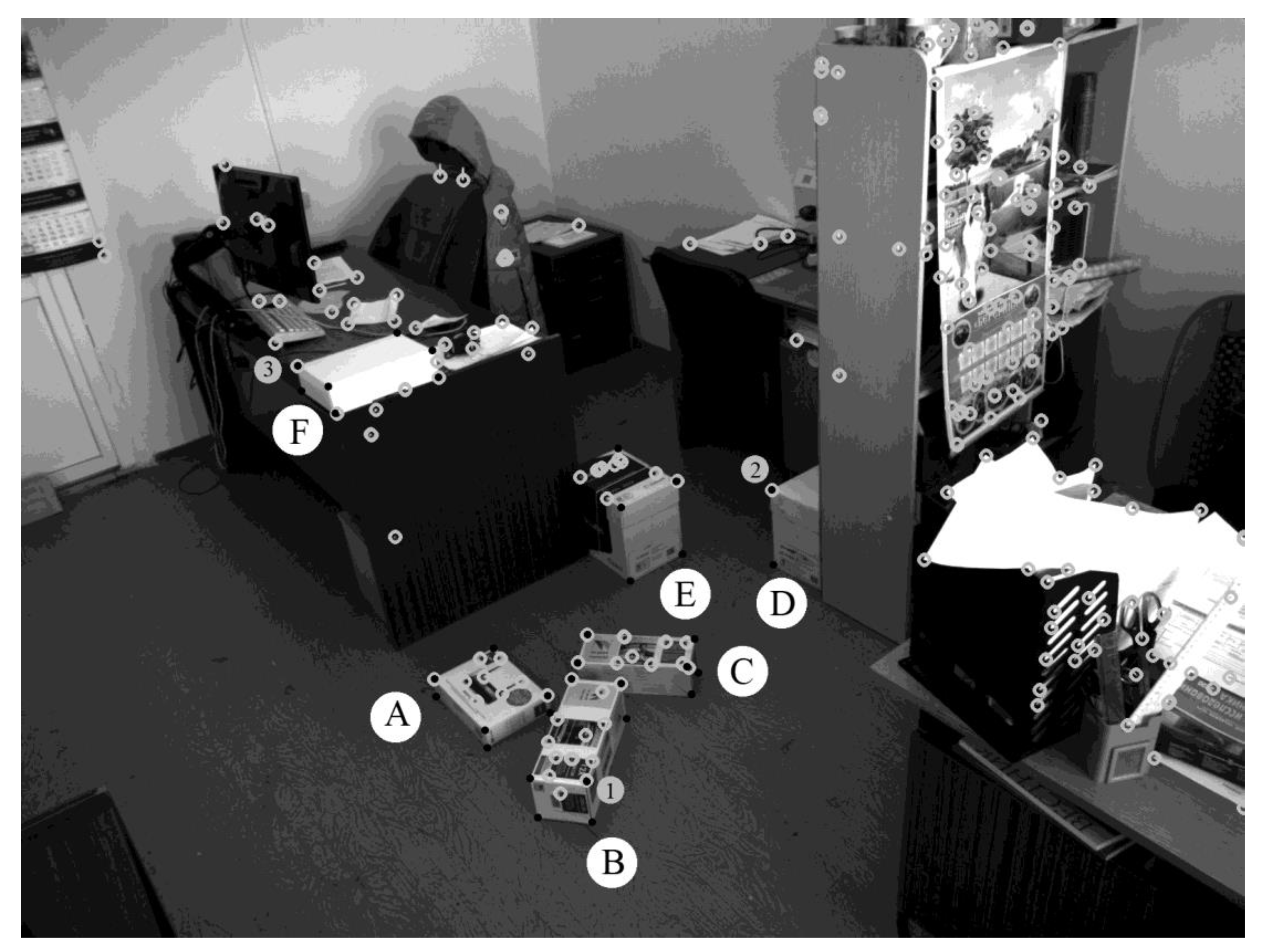
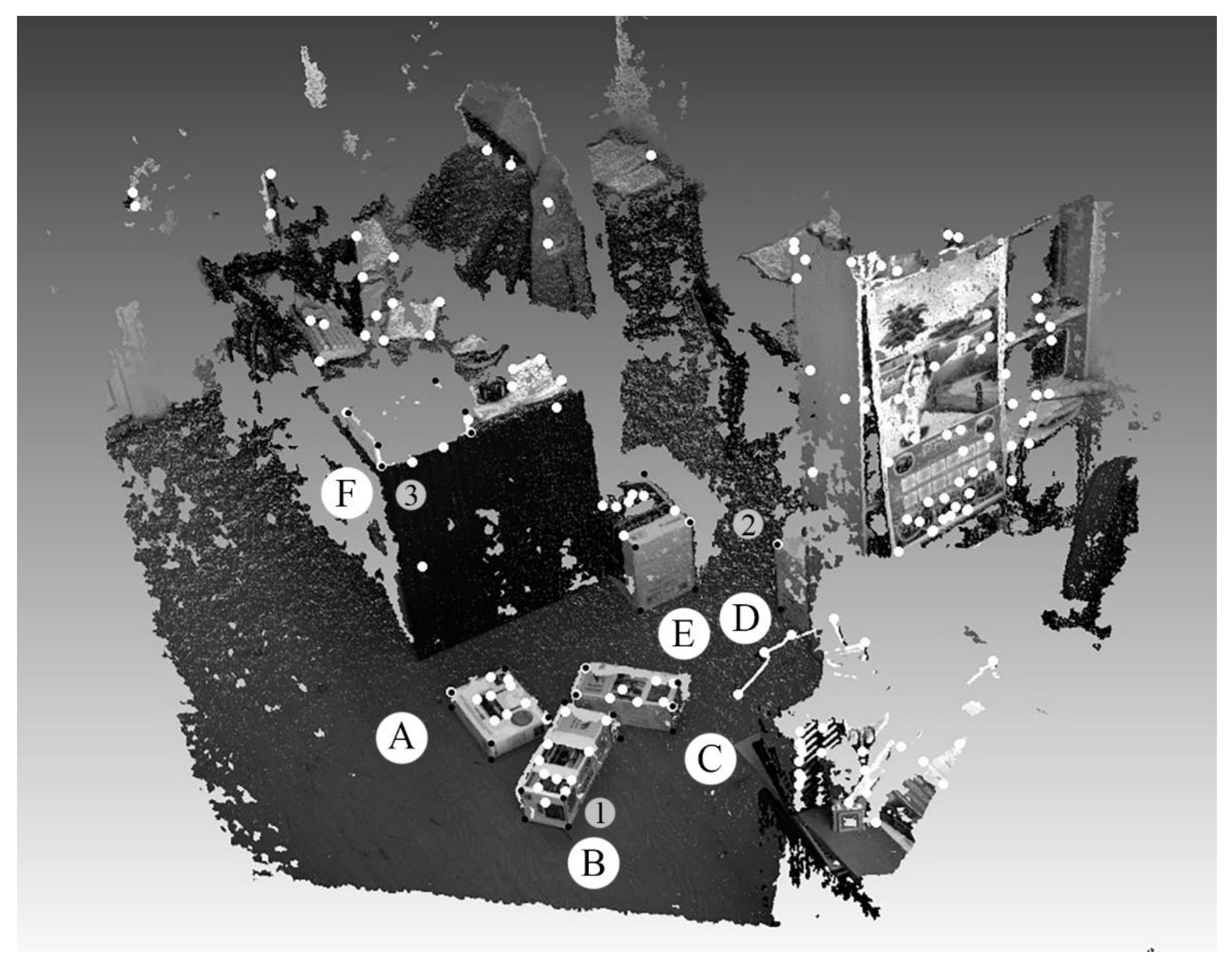
3.2. Experiments with the Karmin2 Camera
3.3. The Discussion of the Results and Comparison with Other Approaches
4. Conclusions
- The object recognition algorithm uses a predetermined 3D point model of the object, in which there are a limited number of characteristic points with known absolute coordinates;
- The method uses a structural coherence criterion when comparing the 3D points of an object with a model;
- The method references the AUV coordinate matrix to the object using the matched points;
- High accuracy during the continuous movement of an AUV in SPS space is ensured by regular referencing to the SPS object coordinate system.
Author Contributions
Funding
Institutional Review Board Statement
Informed Consent Statement
Data Availability Statement
Conflicts of Interest
References
- Mai, C.; Pedersen, S.; Hansen, L.; Jepsen, K.L.; Yang, Z. Subsea infrastructure inspection: A review study. In Proceedings of the 6th International Conference on Underwater System Technology: Theory and Applications, Penang, Malaysia, 13–14 December 2016. [Google Scholar] [CrossRef]
- Zhang, Y.; Zheng, M.; An, C.; Seo, J.K.; Pasqualino, I.; Lim, F.; Duan, M. A review of the integrity management of subsea production systems: Inspection and monitoring methods. Ships Offshore Struct. 2019, 14, 789–803. [Google Scholar] [CrossRef]
- Paull, L.; Saeedi, S.; Seto, M.; Li, H. AUV Navigation and Localization: A Review. IEEE J. Ocean. Eng. 2013, 39, 131–149. [Google Scholar] [CrossRef]
- Terracciano, D.; Bazzarello, L.; Caiti, A.; Costanzi, R.; Manzari, V. Marine Robots for Underwater Surveillance. Curr. Robot. Rep. 2020, 1, 159–167. [Google Scholar] [CrossRef]
- Underwater Inspection System Using an Autonomous Underwater Vehicle (“AUV”) in Combination with a Laser Micro Bathymetry Unit (Triangulation Laser) and High-Definition Camera. Available online: https://patents.google.com/patent/WO2015134473A2 (accessed on 15 September 2021).
- Vidal, E.; Palomeras, N.; Istenič, K.; Hernández, J.D.; Carreras, M. Two-Dimensional Frontier-Based Viewpoint Generation for Exploring and Mapping Underwater Environments. Sensors 2019, 19, 1460. [Google Scholar] [CrossRef] [Green Version]
- Maurelli, F.; Carreras, M.; Salvi, J.; Lane, D.; Kyriakopoulos, K.; Karras, G.; Fox, M.; Long, D.; Kormushev, P.; Caldwell, D. The PANDORA project: A success story in AUV autonomy. In Proceedings of the OCEANS 2016, Shanghai, China, 10–13 April 2016. [Google Scholar]
- Wirth, S.; Carrasco, P.L.N.; Oliver-Codina, G. Visual odometry for autonomous underwater vehicles. In Proceedings of the 2013 MTS/IEEE OCEANS, Bergen, Norway, 10–13 June 2013; pp. 1–6. [Google Scholar] [CrossRef]
- Albiez, J.; Cesar, D.; Gaudig, C.; Arnold, S.; Cerqueira, R.; Trocoli, T.; Mimoso, G.; Saback, R.; Neves, G. Repeated close-distance visual inspections with an AUV. In Proceedings of the OCEANS 2016 MTS/IEEE Monterey, San Diego, CA, USA, 19 September 2016; pp. 1–8. [Google Scholar] [CrossRef]
- Jung, J.; Li, J.-H.; Choi, H.-T.; Myung, H. Localization of AUVs using visual information of underwater structures and artificial landmarks. Intell. Serv. Robot. 2016, 10, 67–76. [Google Scholar] [CrossRef]
- Gao, J.; Wu, P.; Yang, B.; Xia, F. Adaptive neural network control for visual servoing of underwater vehicles with pose estimation. J. Mar. Sci. Technol. 2016, 22, 470–478. [Google Scholar] [CrossRef]
- Xu, H.; Oliveira, P.; Soares, C.G. L1 adaptive backstepping control for path-following of underactuated marine surface ships. Eur. J. Control. 2020, 58, 357–372. [Google Scholar] [CrossRef]
- Fan, S.; Liu, C.; Li, B.; Xu, Y.; Xu, W. AUV docking based on USBL navigation and vision guidance. J. Mar. Sci. Technol. 2018, 24, 673–685. [Google Scholar] [CrossRef]
- Jacobi, M. Autonomous inspection of underwater structures. Robot. Auton. Syst. 2015, 67, 80–86. [Google Scholar] [CrossRef]
- Ferrera, M.; Moras, J.; Trouvé-Peloux, P.; Creuze, V. Real-Time Monocular Visual Odometry for Turbid and Dynamic Underwater Environments. Sensors 2019, 19, 687. [Google Scholar] [CrossRef] [Green Version]
- Zacchini, L.; Bucci, A.; Franchi, M.; Costanzi, R.; Ridolfi, A. Mono visual odometry for Autonomous Underwater Vehicles navigation. In Proceedings of the 2019 OCEANS-Marseille, Marseille, France, 17–20 June 2019; pp. 1–5. [Google Scholar] [CrossRef]
- Sangekar, M.N.; Thornton, B.; Bodenmann, A.; Ura, T. Autonomous Landing of Underwater Vehicles Using High-Resolution Bathymetry. IEEE J. Ocean. Eng. 2019, 45, 1252–1267. [Google Scholar] [CrossRef]
- Himri, K.; Ridao, P.; Gracias, N. 3D Object Recognition Based on Point Clouds in Underwater Environment with Global Descriptors: A Survey. Sensors 2019, 19, 4451. [Google Scholar] [CrossRef] [Green Version]
- Neves, G.; Ruiz, M.; Fontinele, J.; Oliveira, L. Rotated object detection with forward-looking sonar in underwater applications. Expert Syst. Appl. 2019, 140, 112870. [Google Scholar] [CrossRef]
- Nađ, Ð.; Mandić, F.; Mišković, N. Using Autonomous Underwater Vehicles for Diver Tracking and Navigation Aiding. J. Mar. Sci. Eng. 2020, 8, 413. [Google Scholar] [CrossRef]
- González-García, J.; Gómez-Espinosa, A.; Cuan-Urquizo, E.; García-Valdovinos, L.G.; Salgado-Jiménez, T.; Cabello, J.A.E. Autonomous Underwater Vehicles: Localization, Navigation, and Communication for Collaborative Missions. Appl. Sci. 2020, 10, 1256. [Google Scholar] [CrossRef] [Green Version]
- Tamjidi, A.; Ye, C. A pose estimation method for unmanned ground vehicles in GPS denied environments. In Proceedings of the SPIE—The International Society for Optical Engineering, Baltimore, MD, USA, 25 May 2012; pp. 83871K–83871K-12. [Google Scholar] [CrossRef]
- Burguera, A.; Bonin-Font, F.; Oliver, G. Trajectory-Based Visual Localization in Underwater Surveying Missions. Sensors 2015, 15, 1708–1735. [Google Scholar] [CrossRef]
- Papadopoulos, G.; Kurniawati, H.; Shariff, A.S.B.M.; Wong, L.J.; Patrikalakis, N.M. Experiments on Surface Reconstruction for Partially Submerged Marine Structures. J. Field Robot. 2013, 31, 225–244. [Google Scholar] [CrossRef] [Green Version]
- Li, A.Q.; Coskun, A.; Doherty, S.M.; Ghasemlou, S.; Jagtap, A.S.; Modasshir, M.; Rahman, S.; Singh, A.; Xanthidis, M.; O’Kane, J.M.; et al. Experimental Comparison of Open Source Vision-Based State Estimation Algorithms. Int. Symp. Exp. Robot. 2017, 775–786. [Google Scholar] [CrossRef]
- Mur-Artal, R.; Montiel, J.M.M.; Tardos, J. ORB-SLAM: A Versatile and Accurate Monocular SLAM System. IEEE Trans. Robot. 2015, 31, 1147–1163. [Google Scholar] [CrossRef] [Green Version]
- Schonberger, J.L.; Frahm, J.-M. Structure-from-Motion Revisited. In Proceedings of the IEEE Conference on Computer Vision and Pattern Recognition (CVPR), Las Vegas, NV, USA, 27–30 June 2016; pp. 4104–4113. [Google Scholar] [CrossRef]
- Cadena, C.; Carlone, L.; Carrillo, H.; Latif, Y.; Scaramuzza, D.; Neira, J.; Reid, I.; Leonard, J.J. Past, Present, and Future of Simultaneous Localization and Mapping: Toward the Robust-Perception Age. IEEE Trans. Robot. 2016, 32, 1309–1332. [Google Scholar] [CrossRef] [Green Version]
- Vu, M.T.; Le, T.-H.; Thanh, H.L.N.N.; Huynh, T.-T.; Van, M.; Hoang, Q.-D.; Do, T.D. Robust Position Control of an Over-actuated Underwater Vehicle under Model Uncertainties and Ocean Current Effects Using Dynamic Sliding Mode Surface and Optimal Allocation Control. Sensors 2021, 21, 747. [Google Scholar] [CrossRef]
- Vu, M.T.; Choi, H.-S.; Nguyen, N.D.; Kim, S.-K. Analytical design of an underwater construction robot on the slope with an up-cutting mode operation of a cutter bar. Appl. Ocean Res. 2019, 86, 289–309. [Google Scholar] [CrossRef]
- Vu, M.T.; Jeong, S.-K.; Choi, H.-S.; Oh, J.-Y.; Ji, D.-H. Study on down-cutting ladder trencher of an underwater construction robot for seabed application. Appl. Ocean Res. 2018, 71, 90–104. [Google Scholar] [CrossRef]
- Vu, M.T.; Van, M.; Bui, D.H.P.; Do, Q.T.; Huynh, T.-T.; Lee, S.-D.; Choi, H.-S. Study on Dynamic Behavior of Unmanned Surface Vehicle-Linked Unmanned Underwater Vehicle System for Underwater Exploration. Sensors 2020, 20, 1329. [Google Scholar] [CrossRef] [Green Version]
- Vu, M.T.; Choi, H.-S.; Nhat, T.Q.M.; Nguyen, N.D.; Lee, S.-D.; Le, T.-H.; Sur, J. Docking assessment algorithm for autonomous underwater vehicles. Appl. Ocean Res. 2020, 100, 102180. [Google Scholar] [CrossRef]
- Bobkov, V.A.; Kudryashov, A.; Mel’Man, S.V.; Shcherbatyuk, A.F. Autonomous Underwater Navigation with 3D Environment Modeling Using Stereo Images. Gyroscopy Navig. 2018, 9, 67–75. [Google Scholar] [CrossRef]
- Bobkov, V.A.; Kudryashov, A.P.; Inzartsev, A.V. Technology of AUV High-Precision Referencing to Inspected Object. Gyroscopy Navig 2019, 10, 322–329. [Google Scholar] [CrossRef]
- Bobkov, V.A.; Mel’Man, S.V.; Kudryashov, A. Fast computation of local displacement by stereo pairs. Pattern Recognit. Image Anal. 2017, 27, 458–465. [Google Scholar] [CrossRef]
- Melman, S.; Pavin, A.; Bobkov, V.; Inzartsev, A. Distributed simulation framework for investigation of autonomous underwater vehicles’ real-time behavior. In Proceedings of the OCEANS’15 MTS/IEEE, Washington, DC, USA, 19–22 October 2015. [Google Scholar] [CrossRef]
- Pang, G.; Qiu, R.; Huang, J.; You, S.; Neumann, U. Automatic 3D industrial point cloud modeling and recognition. In Proceedings of the 14th IAPR International Conference on Machine Vision Applications (MVA), Tokyo, Japan, 18–22 May 2015; pp. 22–25. [Google Scholar] [CrossRef]
- Guo, Y.; Bennamoun, M.; Sohel, F.; Lu, M.; Wan, J.; Kwok, N.M. A Comprehensive Performance Evaluation of 3D Local Feature Descriptors. Int. J. Comput. Vis. 2015, 116, 66–89. [Google Scholar] [CrossRef]
- Pérez-Alcocer, R.; Torres-Méndez, L.A.; Olguín-Díaz, E.; Maldonado-Ramírez, A.A. Vision-Based Autonomous Underwater Vehicle Navigation in Poor Visibility Conditions Using a Model-Free Robust Control. J. Sensors 2016, 2016, 1–16. [Google Scholar] [CrossRef] [Green Version]


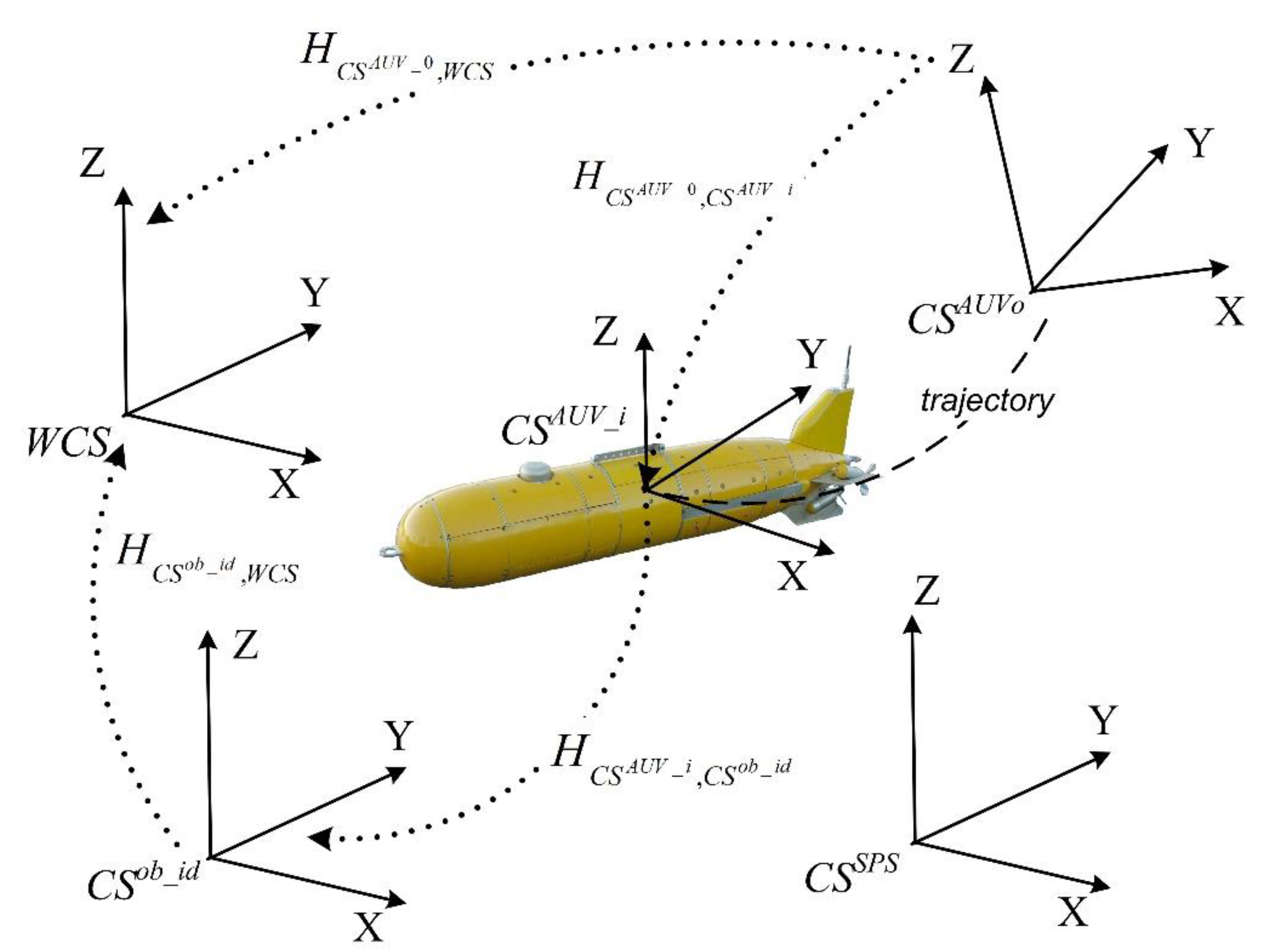
| – | World Coordinate System | |
|---|---|---|
| – | Coordinate system associated with AUV in position i. | |
| – | Coordinate system associated with AUV in the initial position. | |
| – | SPS coordinate system. | |
| – | Coordinate system of object id, belonging to SPS. | |
| – | Transformation matrix from the coordinate system in the initial AUV position to the coordinate system in position i. This matrix is formed by multiplying out local matrices of relative displacement, each of which connects the css of the two adjacent positions. | |
| – | Transformation matrix from the coordinate system of AUV in position i to the coordinate system of object No.id. | |
| – | Transformation matrix from the coordinate system of object id to the world coordinate system. | |
| – | Transformation matrix from the coordinate system of AUV in position 0 to the world coordinate system. |
Publisher’s Note: MDPI stays neutral with regard to jurisdictional claims in published maps and institutional affiliations. |
© 2021 by the authors. Licensee MDPI, Basel, Switzerland. This article is an open access article distributed under the terms and conditions of the Creative Commons Attribution (CC BY) license (https://creativecommons.org/licenses/by/4.0/).
Share and Cite
Bobkov, V.; Kudryashov, A.; Inzartsev, A. Method for the Coordination of Referencing of Autonomous Underwater Vehicles to Man-Made Objects Using Stereo Images. J. Mar. Sci. Eng. 2021, 9, 1038. https://doi.org/10.3390/jmse9091038
Bobkov V, Kudryashov A, Inzartsev A. Method for the Coordination of Referencing of Autonomous Underwater Vehicles to Man-Made Objects Using Stereo Images. Journal of Marine Science and Engineering. 2021; 9(9):1038. https://doi.org/10.3390/jmse9091038
Chicago/Turabian StyleBobkov, Valery, Alexey Kudryashov, and Alexander Inzartsev. 2021. "Method for the Coordination of Referencing of Autonomous Underwater Vehicles to Man-Made Objects Using Stereo Images" Journal of Marine Science and Engineering 9, no. 9: 1038. https://doi.org/10.3390/jmse9091038
APA StyleBobkov, V., Kudryashov, A., & Inzartsev, A. (2021). Method for the Coordination of Referencing of Autonomous Underwater Vehicles to Man-Made Objects Using Stereo Images. Journal of Marine Science and Engineering, 9(9), 1038. https://doi.org/10.3390/jmse9091038