
Ship Trajectory Prediction Based on Bi-LSTM Using Spectral-Clustered AIS Data


Abstract
:1. Introduction
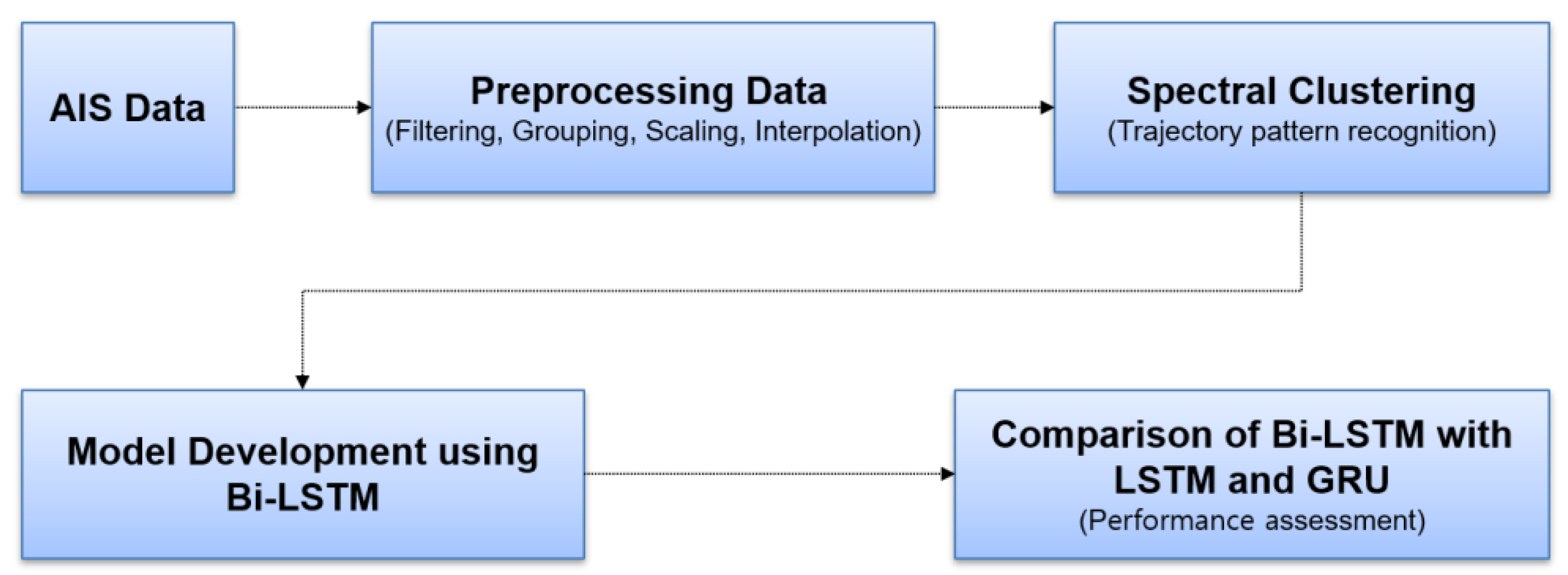
2. Methodology
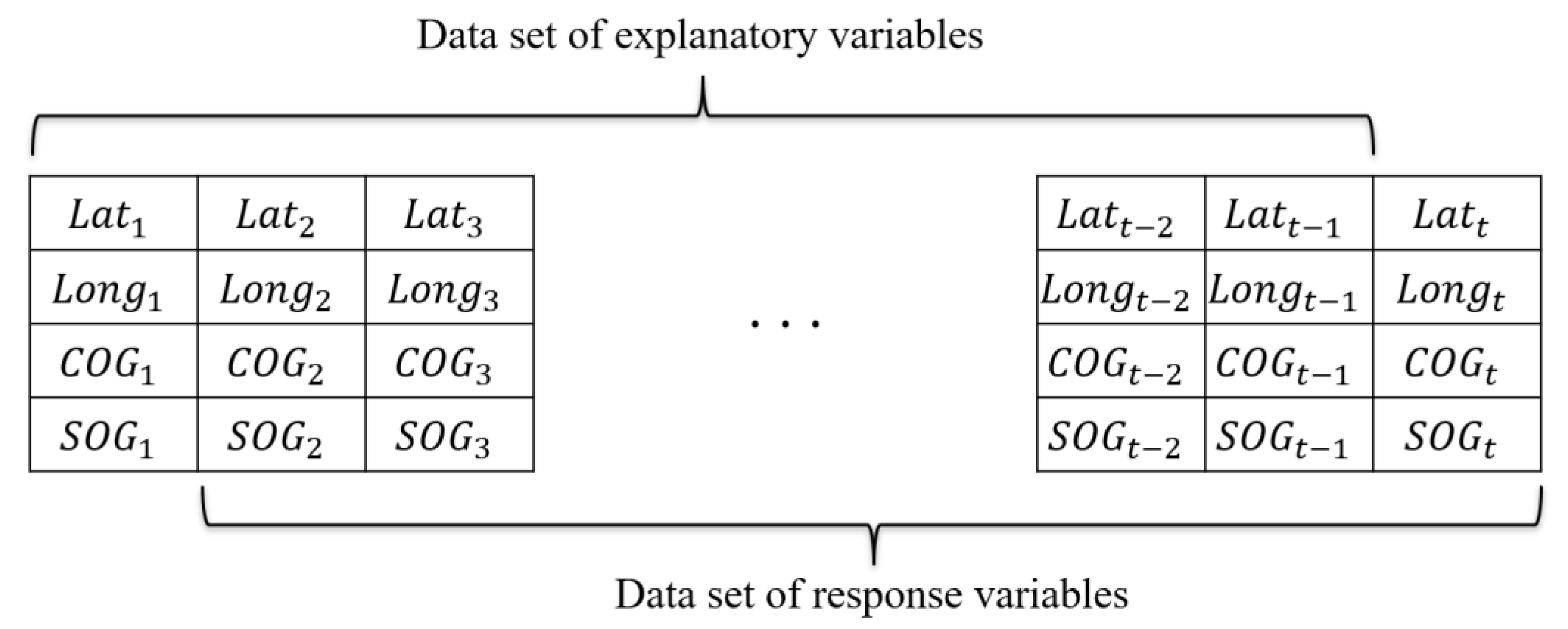
2.1. Preprocessing AIS Data
2.2. Application of Spectral Clustering
2.3. Application of Recurrent Neural Networks
2.3.1. LSTM
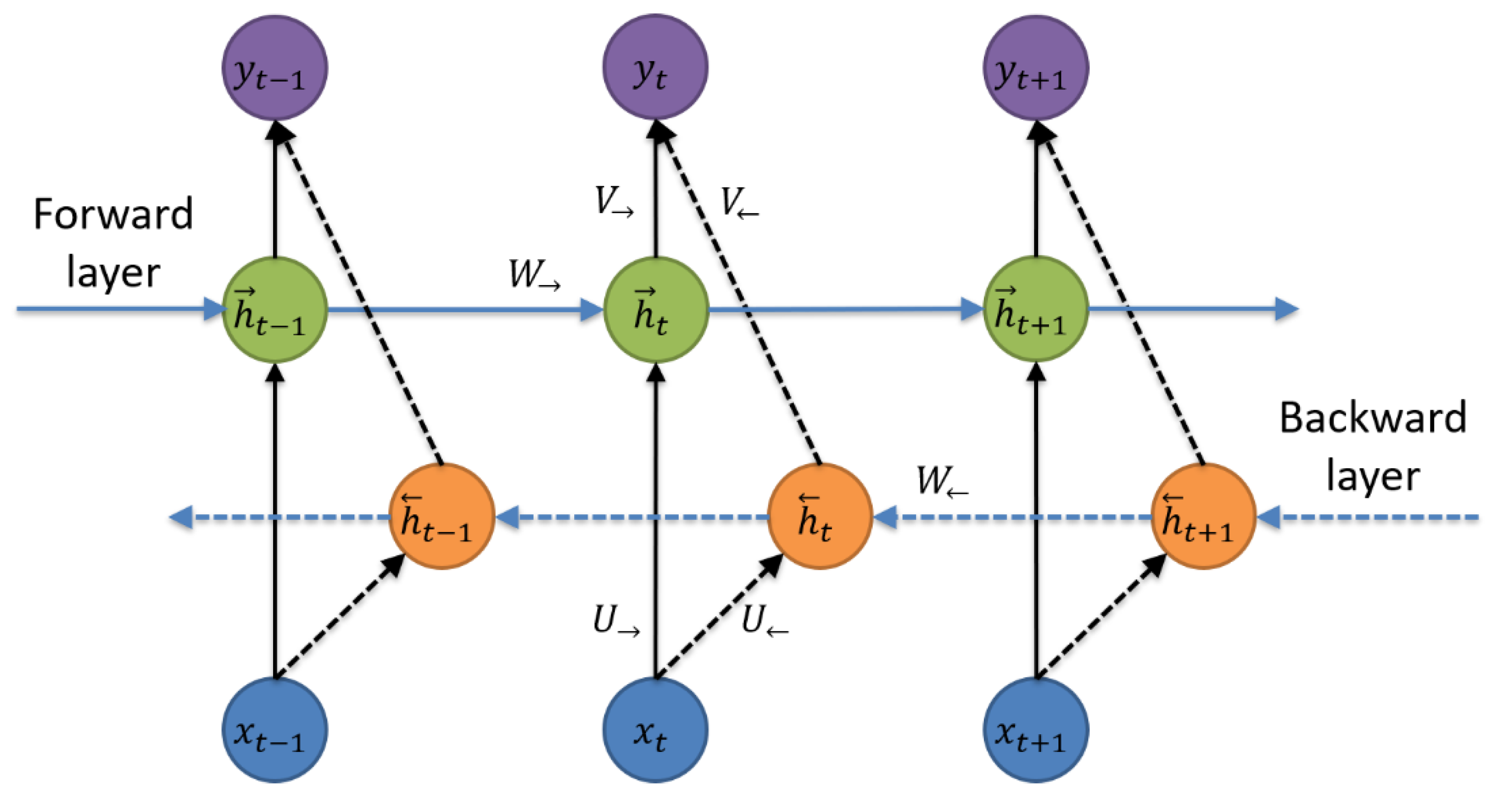
2.3.2. Bi-LSTM
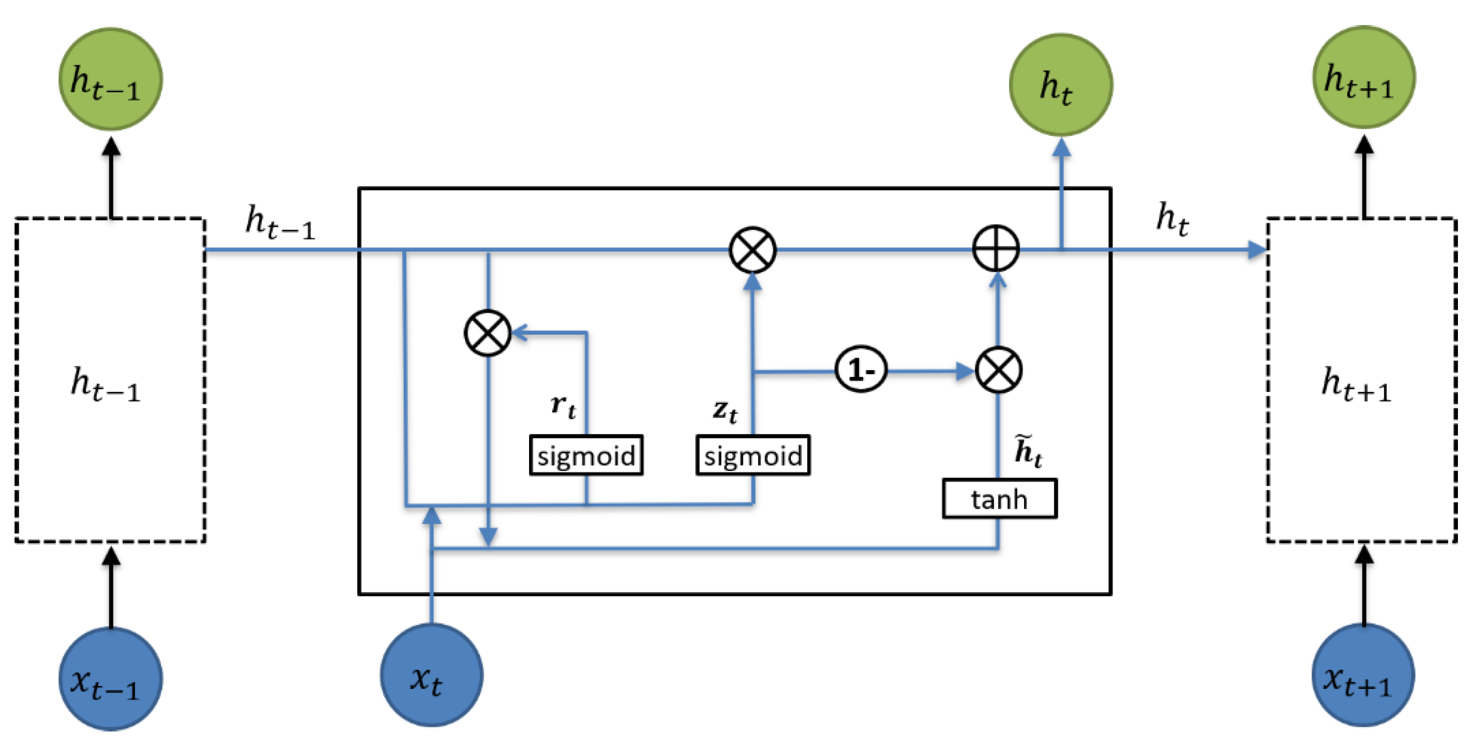
2.3.3. GRU
3. Simulations and Results
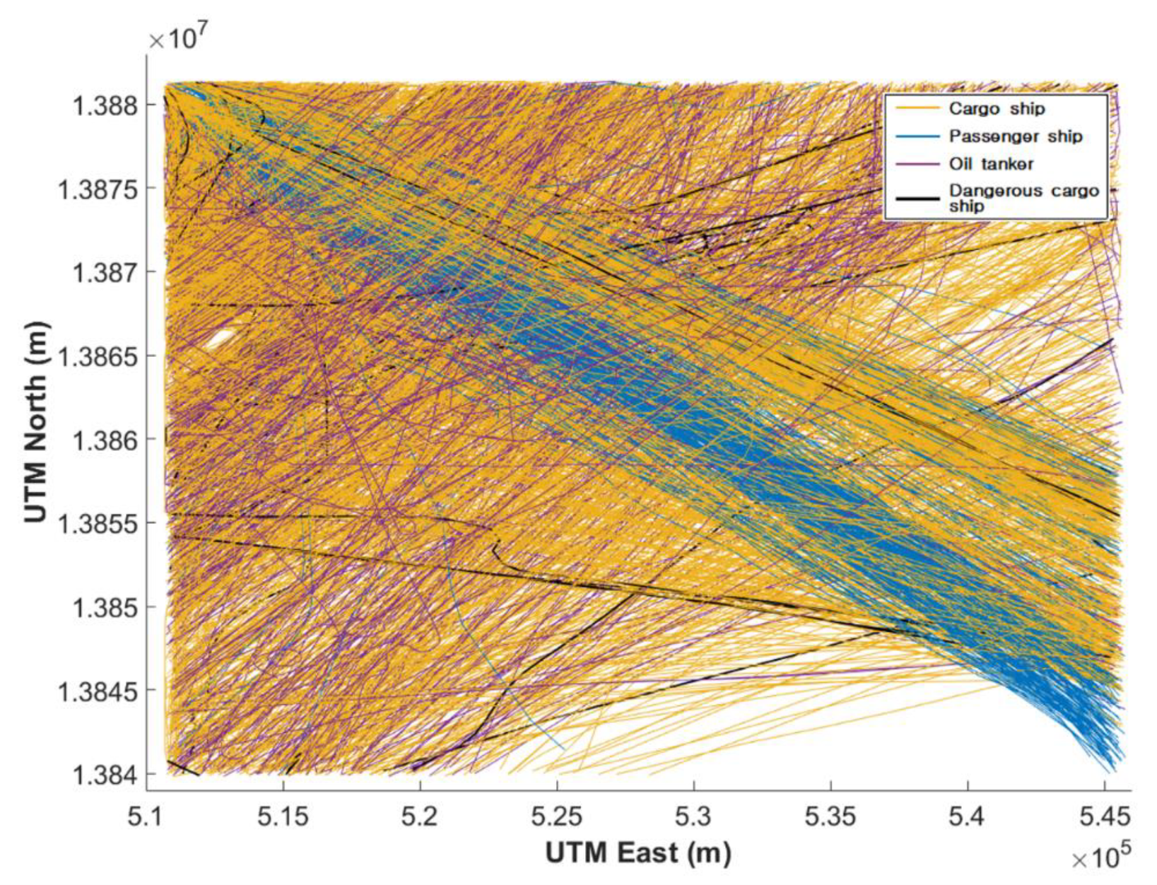
3.1. Data Collection
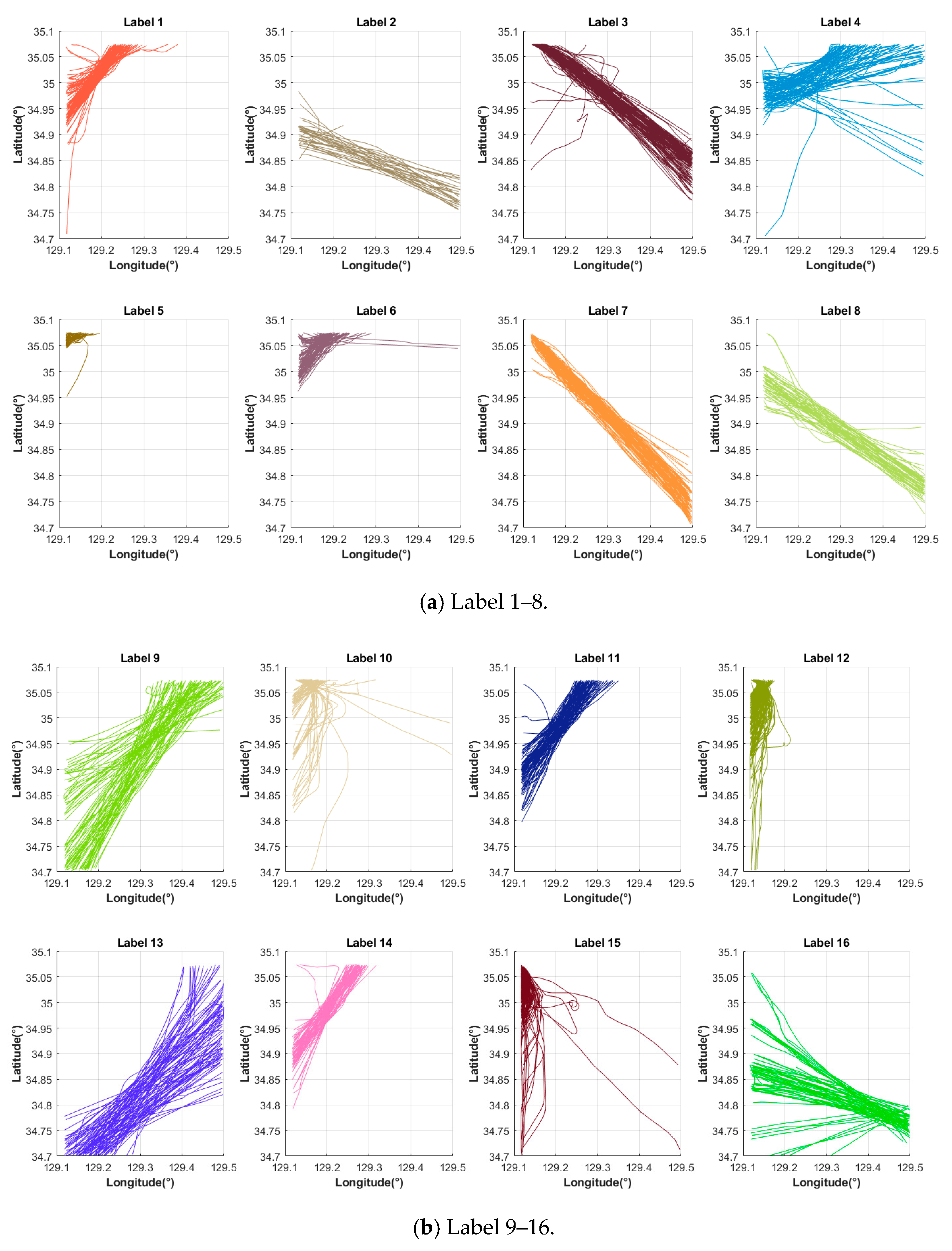
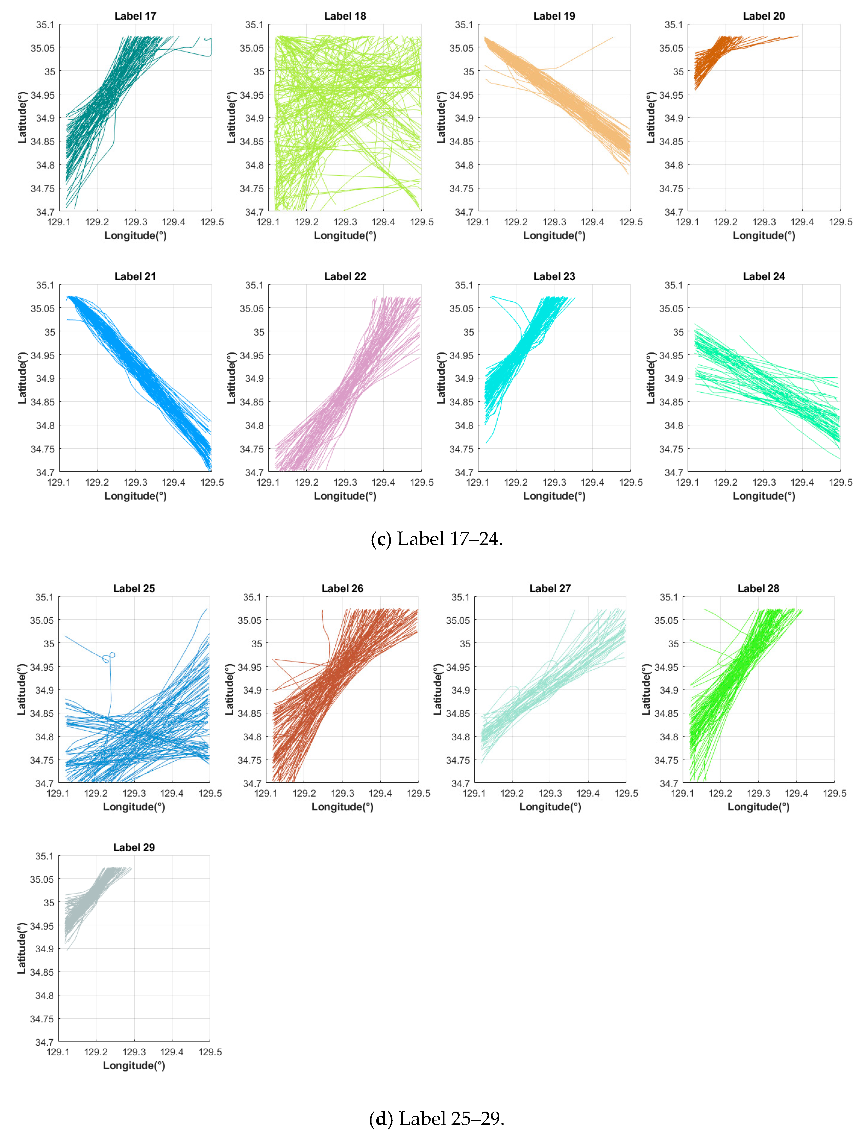
3.2. Results of Ship Trajectory Clustering
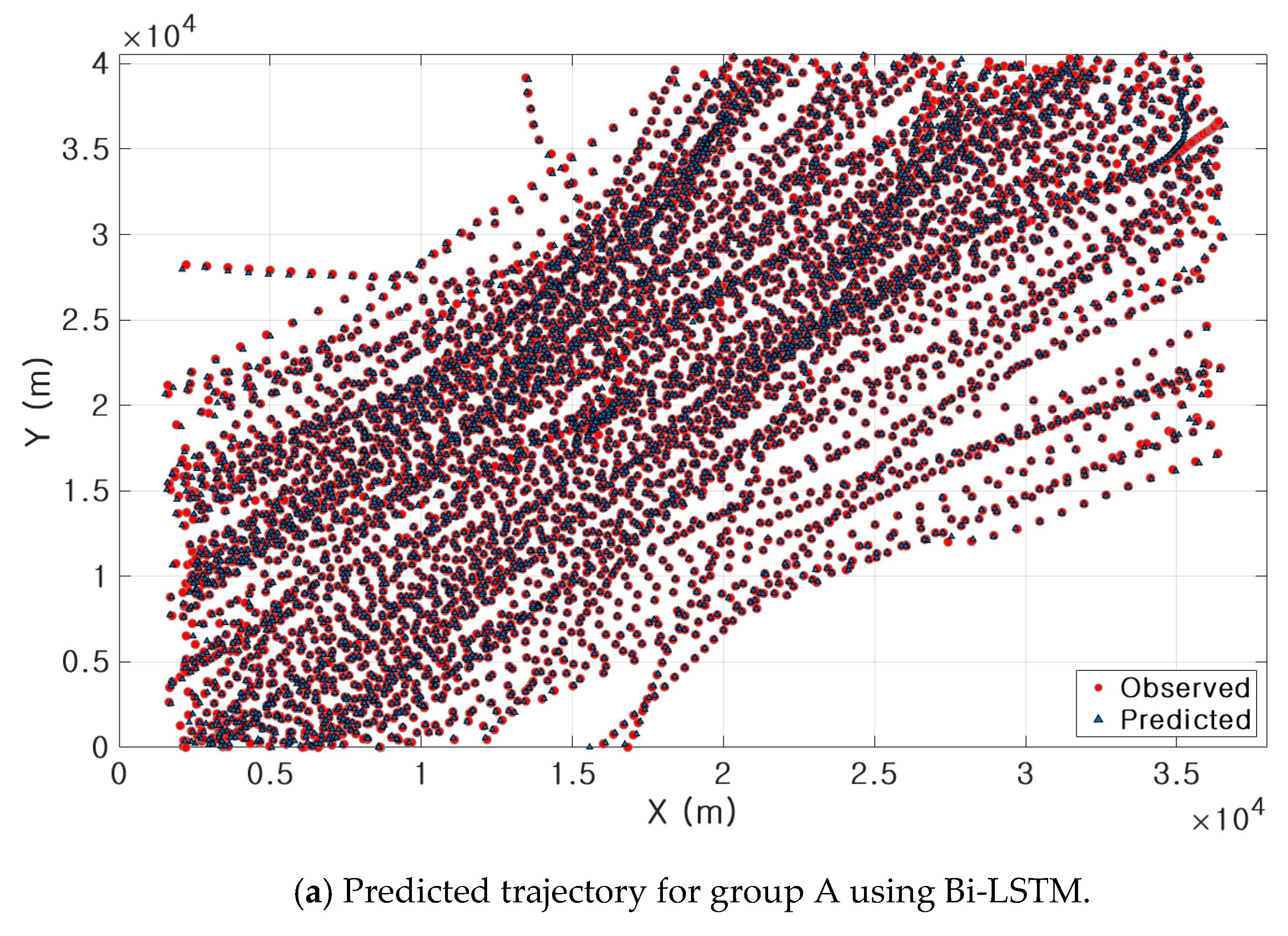
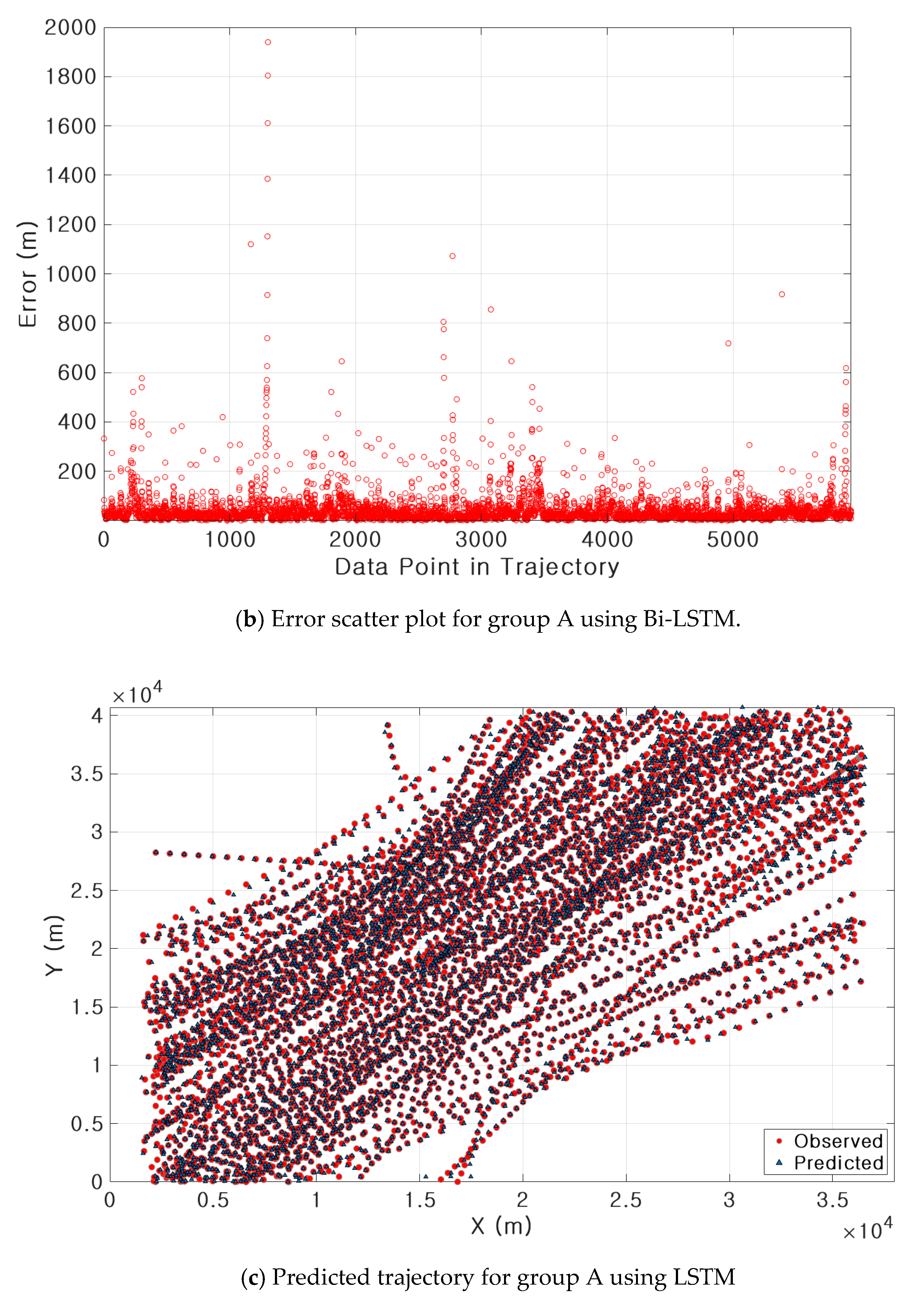
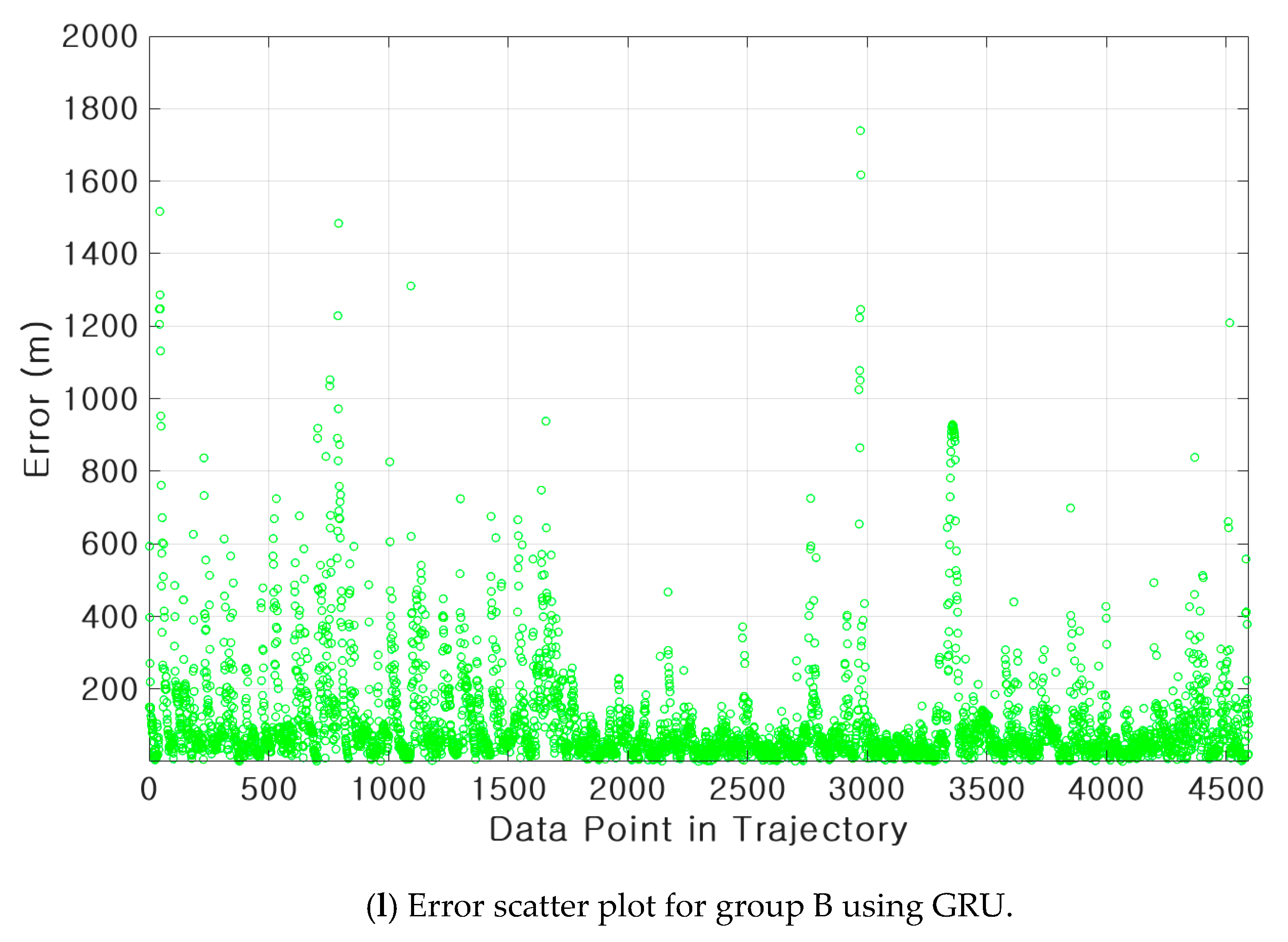
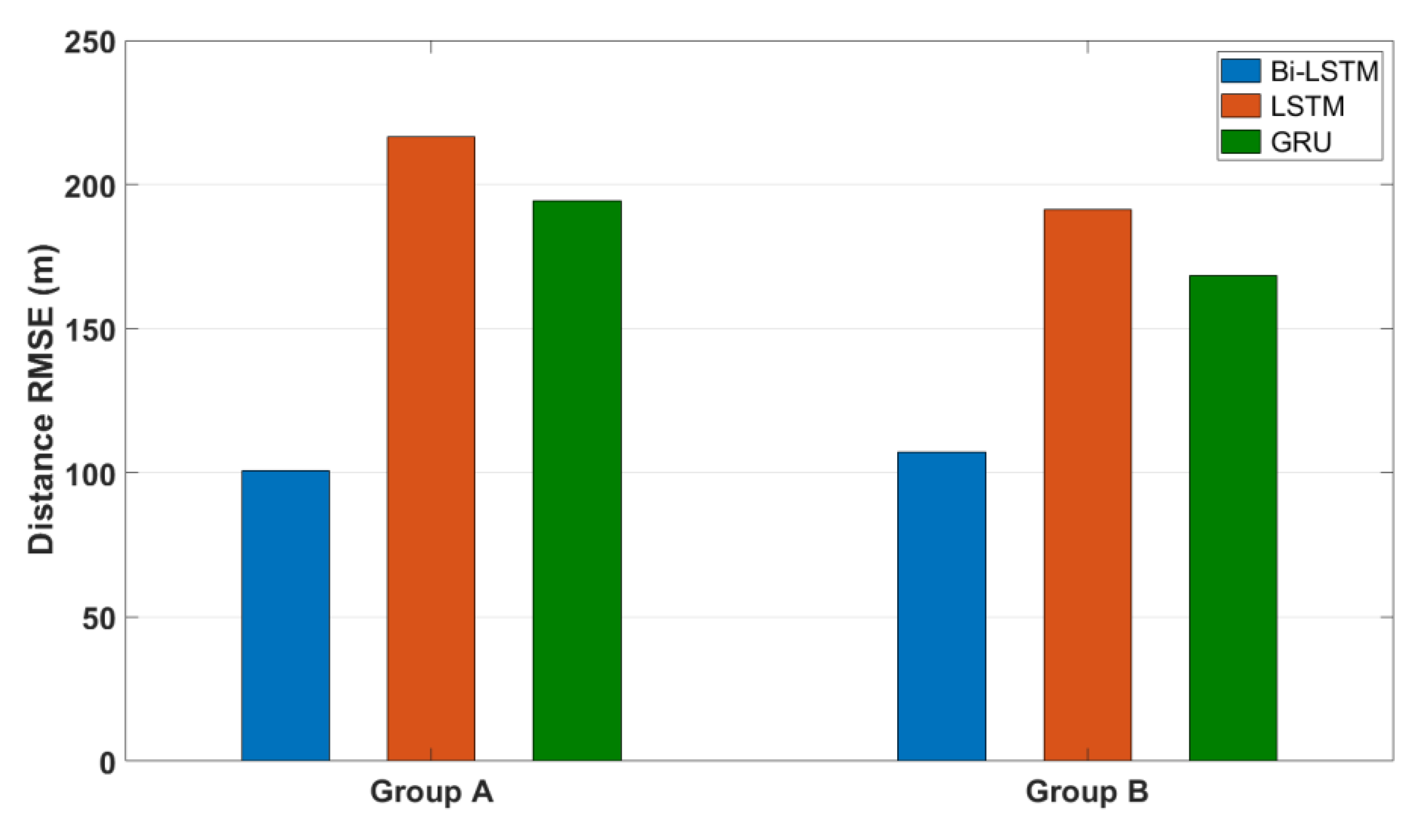
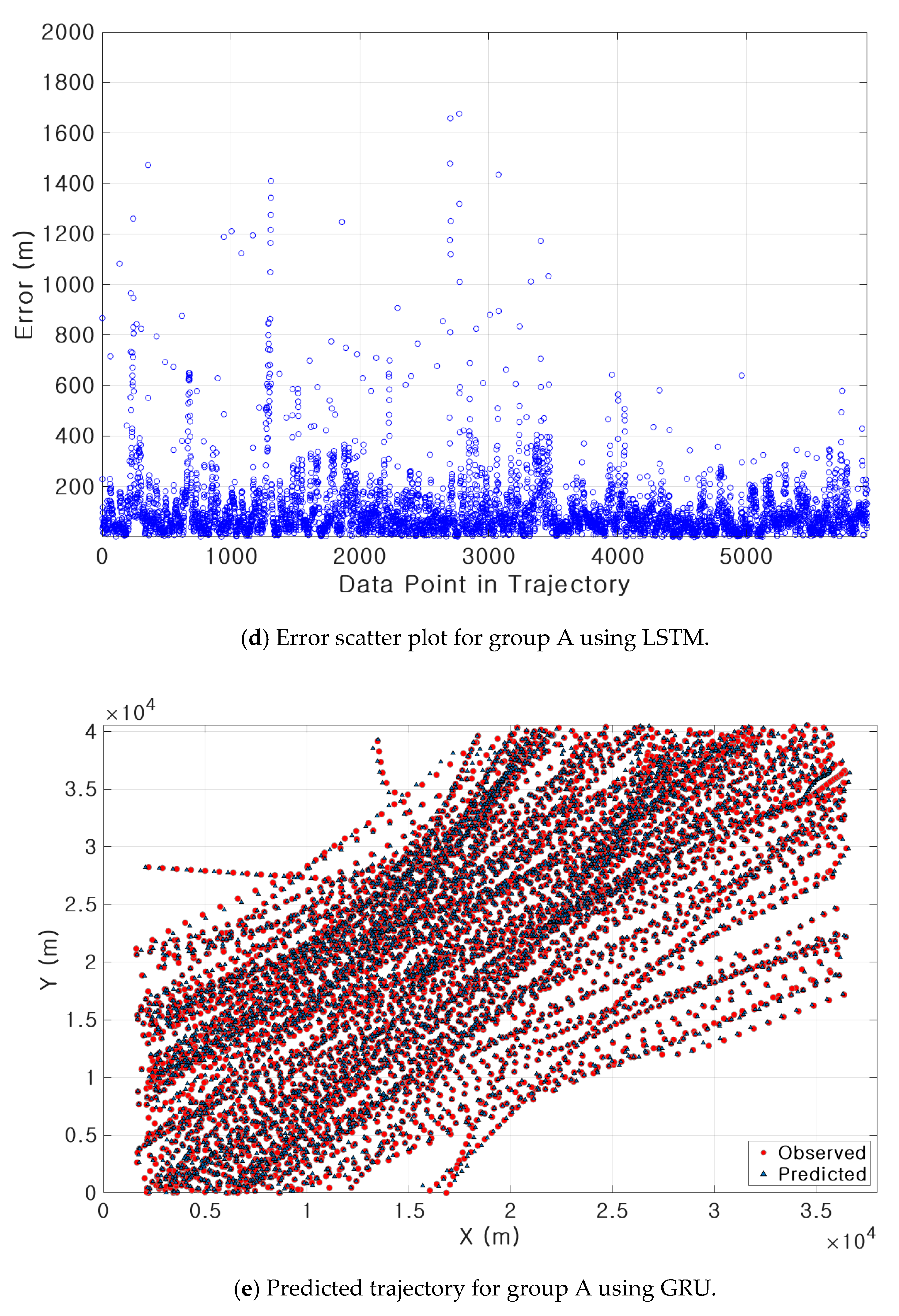
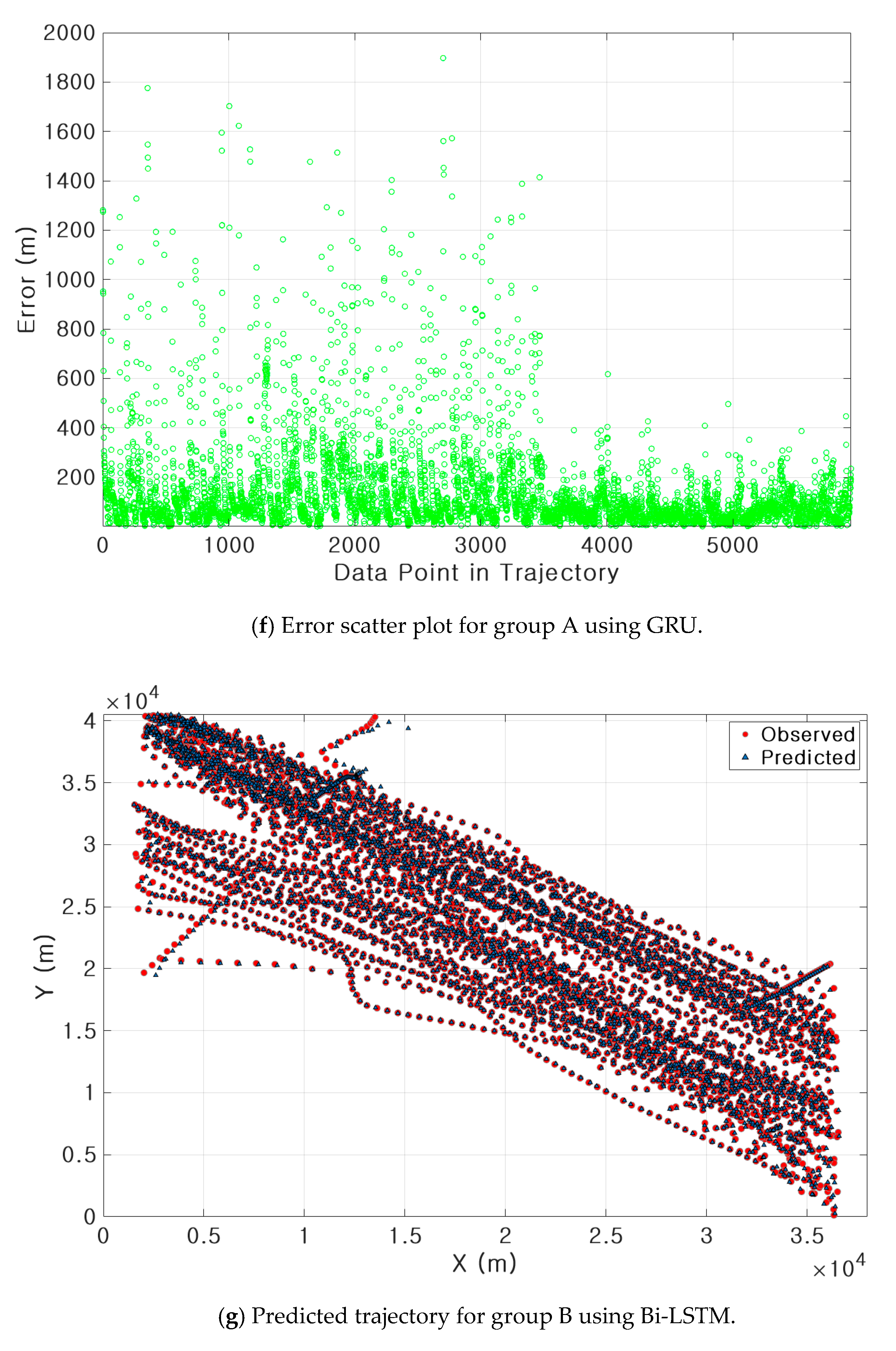
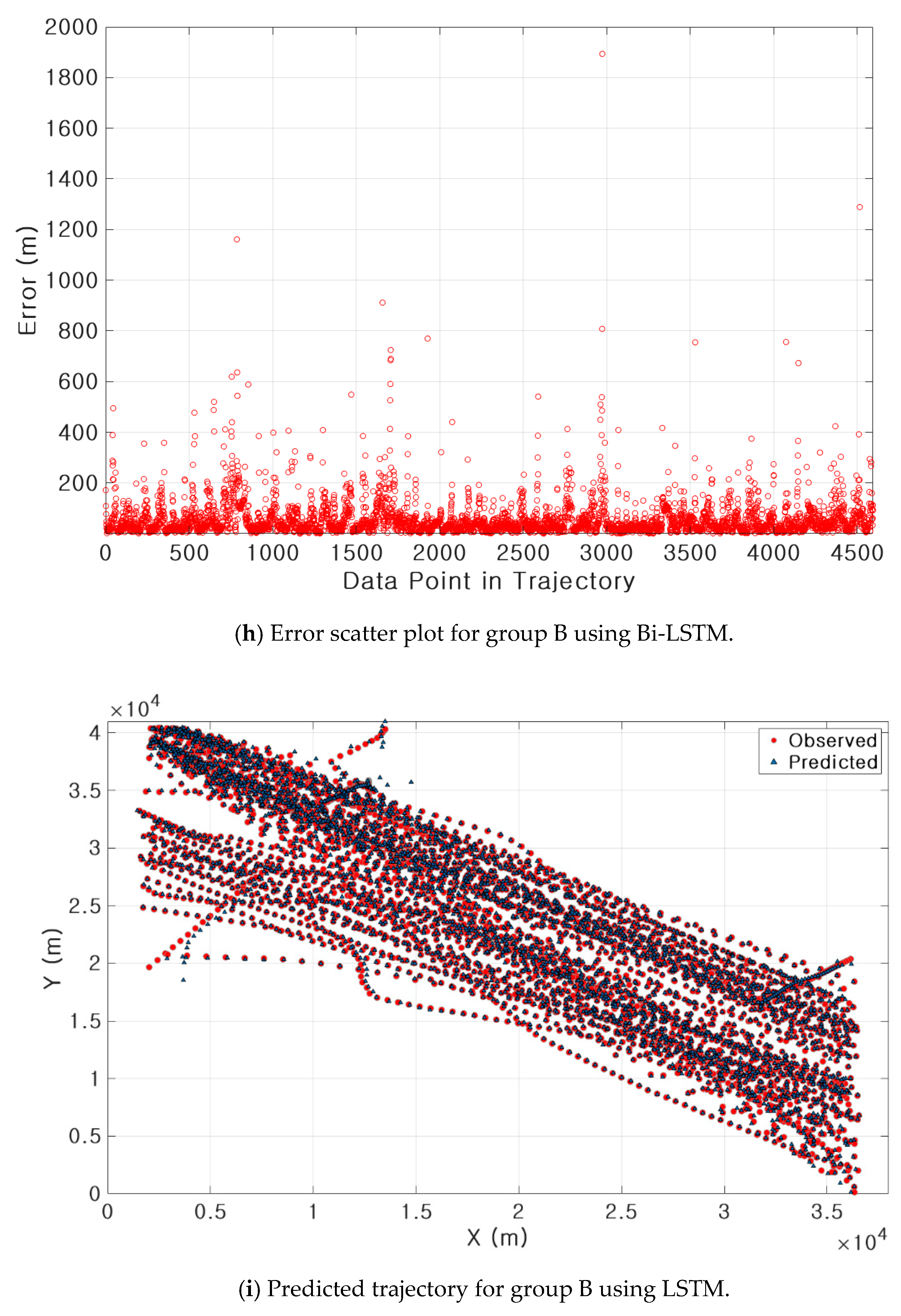
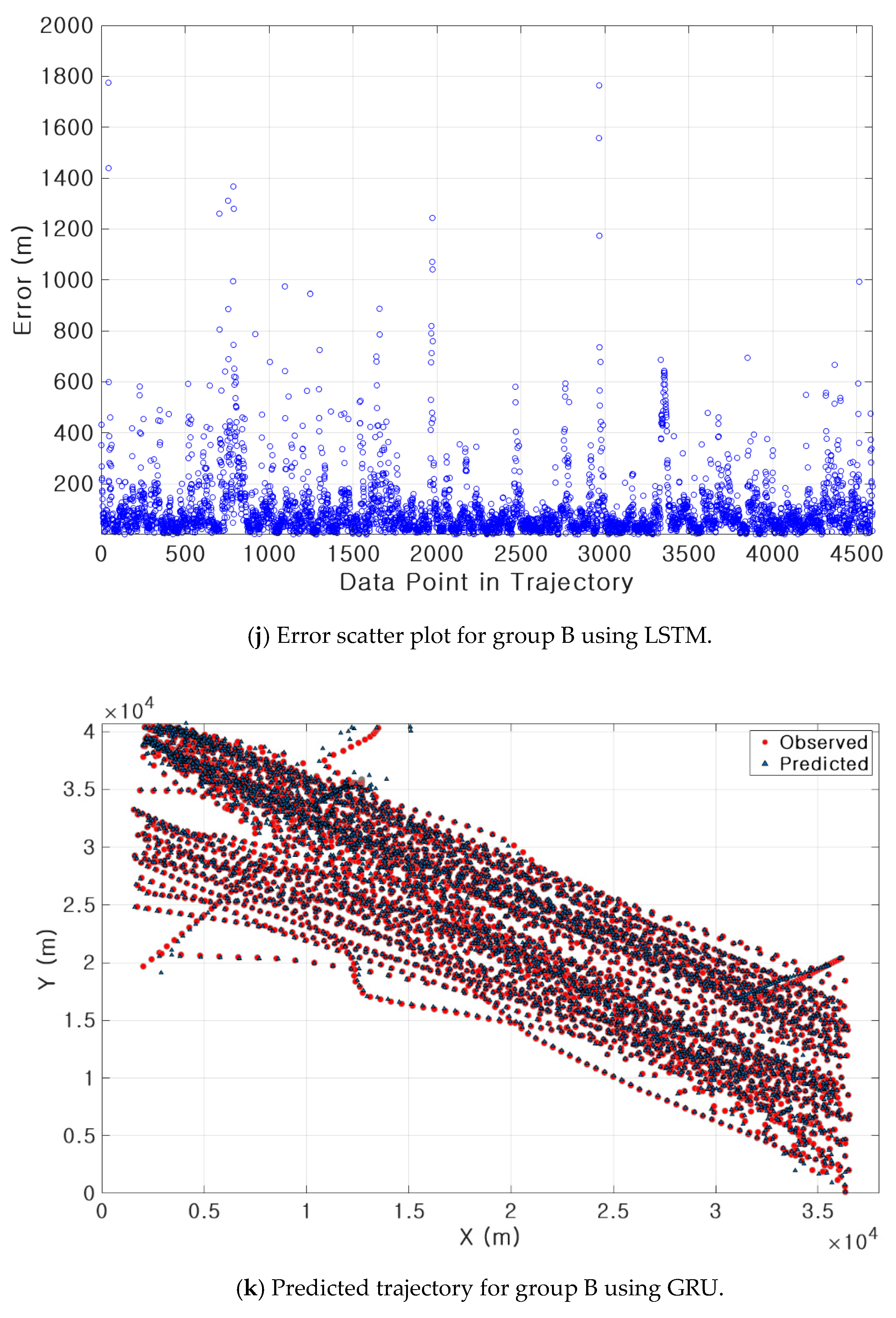
3.3. Results of Ship Trajectory Prediction
4. Conclusions
Author Contributions
Funding
Institutional Review Board Statement
Informed Consent Statement
Data Availability Statement
Conflicts of Interest
References
- KMST (Korean Maritime Safety Tribunal) 2020 Annual Report of Marine Accident Statistics. Available online: https://www.kmst.go.kr (accessed on 3 May 2021).
- McLane, R.C.; Wolf, J.D. Symbolic and Pictorial Displays for Submarine Control. IEEE Trans. Hum. Factors Electron. 1967, HFE-8, 148–158. [Google Scholar] [CrossRef]
- Inoue, S.; Hirano, M.; Kijima, K.; Takashina, J. Practical Calculation Method of Ship Maneuvering Motion. Int. Shipbuild. Prog. 1981, 28, 207–222. [Google Scholar] [CrossRef]
- Fossen, T.I. Handbook of Marine Craft Hydrodynamics and Motion Control; John Wiley & Sons: Chichester, UK, 2011; ISBN 9781119991496. [Google Scholar]
- Passenier, P.O. An Adaptive Track Predictor for Ships. Ph.D. Thesis, Delft University of Technology, Delft, The Netherlands, 1989. [Google Scholar]
- Czapiewska, A.; Sadowski, J. Algorithms for Ship Movement Prediction for Location Data Compression. TransNav Int. J. Mar. Navig. Saf. Sea Transp. 2015, 9, 75–81. [Google Scholar]
- Schöller, C.; Aravantinos, V.; Lay, F.; Knoll, A. What the constant velocity model can teach us about pedestrian motion prediction. IEEE Robot. Autom. Lett. 2020, 5, 1696–1703. [Google Scholar] [CrossRef] [Green Version]
- Johansen, T.A.; Perez, T.; Cristofaro, A. Ship collision avoidance and COLREGS compliance using simulation-based control behavior selection with predictive hazard assessment. IEEE Trans. Intell. Transp. Syst. 2016, 17, 3407–3422. [Google Scholar] [CrossRef] [Green Version]
- Last, P.; Bahlke, C.; Hering-Bertram, M.; Linsen, L. Comprehensive Analysis of Automatic Identification System (AIS) Data in Regard to Vessel Movement Prediction. J. Navig. 2014, 67, 791–809. [Google Scholar] [CrossRef] [Green Version]
- Sang, L.; Yan, X.; Wall, A.; Wang, J.; Mao, Z. CPA calculation method based on AIS position prediction. J. Navig. 2016, 69, 1409–1426. [Google Scholar] [CrossRef]
- van Breda, L.; Passenier, P.O. Effect of path prediction on navigational performance. J. Navig. 1998, 51, 216–228. [Google Scholar] [CrossRef]
- Laxhammar, R. Anomaly detection for sea surveillance. In Proceedings of the 2008 11th International Conference on Information Fusion, Cologne, Germany, 30 June–3 July 2008; IEEE: Piscataway, NJ, USA, 2008; pp. 1–8. [Google Scholar]
- Ristic, B.; La Scala, B.; Morelande, M.; Gordon, N. Statistical analysis of motion patterns in AIS data: Anomaly detection and motion prediction. In Proceedings of the 2008 11th International Conference on Information Fusion, Cologne, Germany, 30 June–3 July 2008; IEEE: Piscataway, NJ, USA, 2008; pp. 1–7. [Google Scholar]
- Aarsæther, K.G.; Moan, T. Estimating navigation patterns from AIS. J. Navig. 2009, 62, 587. [Google Scholar] [CrossRef]
- Tang, H.; Wei, L.; Yin, Y.; Shen, H.; Qi, Y. Detection of abnormal vessel behaviour based on probabilistic directed graph model. J. Navig. 2020, 73, 1014–1035. [Google Scholar] [CrossRef]
- Łącki, M. Intelligent prediction of ship maneuvering. TransNav Int. J. Mar. Navig. Saf. Sea Transp. 2016, 10, 511–516. [Google Scholar] [CrossRef] [Green Version]
- Xu, T.; Liu, X.; Yang, X. Ship Trajectory online prediction based on BP neural network algorithm. In Proceedings of the 2011 International Conference of Information Technology, Computer Engineering and Management Sciences, Nanjing, China, 24–25 September 2011; IEEE: Piscataway, NJ, USA, 2011; Volume 1, pp. 103–106. [Google Scholar]
- Zhou, H.; Chen, Y.; Zhang, S. Ship trajectory prediction based on BP neural network. J. Artif. Intell. 2019, 1, 29. [Google Scholar] [CrossRef]
- Zhao, L.; Shi, G. Maritime anomaly detection using density-based clustering and recurrent neural network. J. Navig. 2019, 72, 894–916. [Google Scholar] [CrossRef]
- Rumelhart, D.E.; Hinton, G.E.; Williams, R.J. Learning representations by back-propagating errors. Nature 1986, 323, 533–536. [Google Scholar] [CrossRef]
- Hochreiter, S.; Schmidhuber, J. Long short-term memory. Neural Comput. 1997, 9, 1735–1780. [Google Scholar] [CrossRef]
- Cho, K.; Van Merriënboer, B.; Gulcehre, C.; Bahdanau, D.; Bougares, F.; Schwenk, H.; Bengio, Y. Learning phrase representations using RNN encoder-decoder for statistical machine translation. arXiv 2014, arXiv:1406.1078. [Google Scholar]
- Shi, Z.; Pan, Q.; Xu, M. LSTM-Cubic A*-based auxiliary decision support system in air traffic management. Neurocomputing 2020, 391, 167–176. [Google Scholar] [CrossRef]
- Graves, A.; Schmidhuber, J. Framewise phoneme classification with bidirectional LSTM and other neural network architectures. Neural Netw. 2005, 18, 602–610. [Google Scholar] [CrossRef]
- Siami-Namini, S.; Tavakoli, N.; Namin, A.S. The performance of LSTM and BiLSTM in forecasting time series. In Proceedings of the 2019 IEEE International Conference on Big Data (Big Data), Los Angeles, CA, USA, 9–12 December 2019; IEEE: Piscataway, NJ, USA, 2019; pp. 3285–3292. [Google Scholar]
- Riveiro, M.; Pallotta, G.; Vespe, M. Maritime anomaly detection: A review. Wiley Interdiscip. Rev. Data Min. Knowl. Discov. 2018, 8, e1266. [Google Scholar] [CrossRef] [Green Version]
- Ester, M.; Kriegel, H.-P.; Sander, J.; Xu, X. A density-based algorithm for discovering clusters in large spatial databases with noise. In Proceedings of the Second International Conference on Knowledge Discovery and Data Mining, Portland, OR, USA, 2–4 August 1996; Volume 96, pp. 226–231. [Google Scholar]
- Vlachos, M.; Kollios, G.; Gunopulos, D. Discovering similar multidimensional trajectories. In Proceedings of the 18th International Conference on Data Engineering, San Jose, CA, USA, 26 February–1 March 2002; IEEE: Piscataway, NJ, USA, 2002; pp. 673–684. [Google Scholar]
- IMO (International Maritime Organization). Adoption of New and Amended Performance Standards for Navigational Equipment; IMO: London, UK, 1998; Volume 86, pp. 13–16. [Google Scholar]
- Sang, L.Z.; Yan, X.P.; Mao, Z.; Ma, F. Restoring method of vessel track based on AIS information. In Proceedings of the 11th International Symposium on Distributed Computing and Applications to Business, Engineering & Science, Guilin, China, 19–22 October 2012; pp. 336–340. [Google Scholar] [CrossRef]
- Zhang, D.; Li, J.; Wu, Q.; Liu, X.; Chu, X.; He, W. Enhance the AIS data availability by screening and interpolation. In Proceedings of the 2017 4th International Conference on Transportation Information and Safety (ICTIS), Banff, AB, Canada, 8–10 August 2017; pp. 981–986. [Google Scholar] [CrossRef] [Green Version]
- Shi, Z.; Xu, M.; Pan, Q.; Yan, B.; Zhang, H. LSTM-based flight trajectory prediction. In Proceedings of the 2018 International Joint Conference on Neural Networks (IJCNN), Rio de Janeiro, Brazil, 8–13 July 2018; IEEE: Piscataway, NJ, USA, 2018; pp. 1–8. [Google Scholar]
- Morris, B.T. Understanding Activity from Trajectory Patterns. Ph.D. Thesis, University of California San Diego, La Jolla, CA, USA, 2010. [Google Scholar]
- Shi, J.; Malik, J. Normalized cuts and image segmentation. IEEE Trans. Pattern Anal. Mach. Intell. 2000, 22, 888–905. [Google Scholar]
- Von Luxburg, U. A tutorial on spectral clustering. Stat. Comput. 2007, 17, 395–416. [Google Scholar] [CrossRef]
- Ng, A.; Jordan, M.; Weiss, Y. On spectral clustering: Analysis and an algorithm. Adv. Neural Inf. Process. Syst. 2001, 14, 849–856. [Google Scholar]
- Lloyd, S. Least squares quantization in PCM. IEEE Trans. Inf. Theory 1982, 28, 129–137. [Google Scholar] [CrossRef]
- Gers, F.A.; Schmidhuber, J.; Cummins, F. Learning to forget: Continual prediction with LSTM. IEE Conf. Publ. 1999, 2, 850–855. [Google Scholar] [CrossRef]
- Schuster, M.; Paliwal, K.K. Bidirectional recurrent neural networks. IEEE Trans. Signal Process. 1997, 45, 2673–2681. [Google Scholar] [CrossRef] [Green Version]
- Park, J.; Jeong, J.S. An Estimation of Ship Collision Risk Based on Relevance Vector Machine. J. Mar. Sci. Eng. 2021, 9, 538. [Google Scholar] [CrossRef]
- Ministry of Oceans and Fisheries. Statistics of Vessels Arrival and Departure at Major Port of Korea. Available online: http://www.mof.go.kr (accessed on 3 May 2021).
- Park, J. A Study on the Estimation of Ship Collision Risk Using Machine Learning and Its Optimal Path Finding. Ph.D. Thesis, Mokpo National Maritime University, Mokpo, Korea, 2021. [Google Scholar]


| Label | Quantity | Ratio (%) | Label | Quantity | Ratio (%) | Label | Quantity | Ratio (%) |
|---|---|---|---|---|---|---|---|---|
| 1 | 104 | 3.69 | 11 | 104 | 3.69 | 21 | 89 | 3.16 |
| 2 | 33 | 1.17 | 12 | 215 | 7.63 | 22 | 75 | 2.66 |
| 3 | 124 | 4.40 | 13 | 94 | 3.34 | 23 | 88 | 3.13 |
| 4 | 102 | 3.62 | 14 | 80 | 2.84 | 24 | 62 | 2.20 |
| 5 | 77 | 2.73 | 15 | 195 | 6.92 | 25 | 100 | 3.55 |
| 6 | 108 | 3.84 | 16 | 64 | 2.27 | 26 | 102 | 3.62 |
| 7 | 101 | 3.59 | 17 | 75 | 2.66 | 27 | 51 | 1.81 |
| 8 | 58 | 2.06 | 18 | 165 | 5.86 | 28 | 81 | 2.88 |
| 9 | 87 | 3.09 | 19 | 101 | 3.59 | 29 | 121 | 4.30 |
| 10 | 85 | 3.02 | 20 | 75 | 2.67 | - | - | - |
| Group | Cluster Label | Direction | Quantity |
|---|---|---|---|
| A | 9, 13, 17, 22, 26, 27, 28 | Northeast/Southwest | 565 (20.1%) |
| B | 3, 7, 8, 19, 21, 24 | Northwest/Southeast | 535 (19.0%) |
| Group | Method | Avg. Elapsed Training Time | ||||
|---|---|---|---|---|---|---|
| Distance | Course | Speed | ||||
| A | Bi-LSTM | 22 min 1 s | 0.0104 (101 m) | 0.0345 (3.1°) | 0.0275 (0.1 knot) | 0.26 |
| LSTM | 9 min 8 s | 0.0224 (217 m) | 0.1495 (13.4°) | 0.1042 (0.3 knot) | 1.00 | |
| GRU | 8 min 20 s | 0.0202 (194 m) | 0.1464 (13.1°) | 0.1041 (0.3 knot) | 0.98 | |
| B | Bi-LSTM | 22 min 26 s | 0.0113 (107 m) | 0.0219 (2.0°) | 0.0219 (0.2 knot) | 0.27 |
| LSTM | 9 min 45 s | 0.0201 (191 m) | 0.1242 (11.4°) | 0.0583 (0.6 knot) | 1.00 | |
| GRU | 8 min 24 s | 0.0177 (169 m) | 0.1251 (11.49°) | 0.0583 (0.6 knot) | 0.99 | |
Publisher’s Note: MDPI stays neutral with regard to jurisdictional claims in published maps and institutional affiliations. |
© 2021 by the authors. Licensee MDPI, Basel, Switzerland. This article is an open access article distributed under the terms and conditions of the Creative Commons Attribution (CC BY) license (https://creativecommons.org/licenses/by/4.0/).
Share and Cite
Park, J.; Jeong, J.; Park, Y. Ship Trajectory Prediction Based on Bi-LSTM Using Spectral-Clustered AIS Data. J. Mar. Sci. Eng. 2021, 9, 1037. https://doi.org/10.3390/jmse9091037
Park J, Jeong J, Park Y. Ship Trajectory Prediction Based on Bi-LSTM Using Spectral-Clustered AIS Data. Journal of Marine Science and Engineering. 2021; 9(9):1037. https://doi.org/10.3390/jmse9091037
Chicago/Turabian StylePark, Jinwan, Jungsik Jeong, and Youngsoo Park. 2021. "Ship Trajectory Prediction Based on Bi-LSTM Using Spectral-Clustered AIS Data" Journal of Marine Science and Engineering 9, no. 9: 1037. https://doi.org/10.3390/jmse9091037
APA StylePark, J., Jeong, J., & Park, Y. (2021). Ship Trajectory Prediction Based on Bi-LSTM Using Spectral-Clustered AIS Data. Journal of Marine Science and Engineering, 9(9), 1037. https://doi.org/10.3390/jmse9091037