Article

A Heuristic Approach for Inter-Facility Comparison of Results from Round Robin Testing of a Floating Wind Turbine in Irregular Waves

1
MaREI Centre, Environmental Research Institute, University College Cork, P43 C573 Cork, Ireland
2
Ifremer, Laboratoire Comportement des Structures en Mer, CS 10070, 29280 Plouzane, France
3
École Centrale de Nantes, LHEEA Laboratory, 44000 Nantes, France
4
Department of Naval Architecture, Ocean and Marine Engineering, University of Strathclyde, 100 Montrose Street, Glasgow G4 0LZ, UK
*
Authors to whom correspondence should be addressed.
J. Mar. Sci. Eng. 2021, 9(9), 1030; https://doi.org/10.3390/jmse9091030
Submission received: 5 August 2021 / Revised: 13 September 2021 / Accepted: 15 September 2021 / Published: 18 September 2021
(This article belongs to the Special Issue Marine Renewables–Infrastructures and Physical Testing)

Abstract

:
This paper introduces metrics developed for analysing irregular wave test results from the round robin testing campaign carried out on a floating wind turbine as part of the EU H2020 MaRINET2 project. A 1/60th scale model of a 10 MW floating platform was tested in wave basins in four different locations around Europe. The tests carried out in each facility included decay tests, tests in regular and irregular waves with and without wind thrust, and tests to characterise the mooring system as well as the model itself. While response amplitude operations (RAOs) are a useful tool for assessing device performance in irregular waves, they are not easy to interpret when performing an inter-facility comparison where there are many variables. Metrics that use a single value per test condition rather than an RAO curve are a means of efficiently comparing tests from different basins in a more heuristic manner. In this research, the focus is on using metrics to assess how the platform responds with varying wave height and thrust across different facilities. It is found that the metrics implemented are very useful for extracting global trends across different basins and test conditions.

1. Introduction

One of the key aims of the EU H2020 MaRINET2 project1 is to improve the quality, robustness, and accuracy of laboratory testing of ocean energy devices. Scaled model testing in a laboratory is an integral part of the development process for many offshore renewable energy (ORE) technologies. Testing at small scale can be efficient and relatively inexpensive, while testing within a controlled environment enables experiments to be repeated for a range of parameters.
Testing a floating wind platform at reduced scale typically involves still water decay tests, tests in regular and irregular waves with and without wind emulation, tests to characterise the mooring system, and tests on dry land that characterise the model itself, e.g., the moments of inertia (MoI) and the centre of gravity (CoG). During tank testing, motions of the model in each of the six degrees of freedom (DoF), i.e., surge, sway, heave, roll, yaw, and pitch, are measured to determine how the platform responds to a range of wind and wave conditions. Generating this data allows validation of numerical models and characterisation of the dynamics of a full-scale platform. In short, model testing is often the first opportunity to carry out a simplified, but global, assessment of the moored platform and the turbine together [1].
However, the effect that the facility used for the model tests will have on the outcomes is uncertain, even when following the same methodologies for carrying out the tests which is not often the case. Research carried out within MaRINET2 [2,3] identified a shortfall in the published guidance available for conducting laboratory testing of floating offshore wind turbines. Much of the existing literature is derived form the oil and gas industry and published by the International Towing Tank Conference (ITTC) literature that deals with ocean engineering2.
To investigate the effect of the facility, a round robin testing program was executed in MaRINET2 whereby generic wave, floating wind, and tidal devices were tested in different infrastructures. The wave [4,5,6] and wind [7] round robin testing included many tests in waves. One of main lessons learnt from this exercise is that it is not straightforward to compare results of wave tests obtained from different basins. Linear response amplitude operators (RAOs) were found valuable for a first comparison [7]. However, the impossibility of generating identical waves in two distinct basins combined with the fact that responses to waves are not fully linear bring an additional challenge for a cross-facility comparison. One way to work around this obstacle is to find metrics which are less sensitive to differences between wave realisations. This paper proposes a set of metrics facilitating the comparison of results from different facilities in irregular waves. It develops the application of these metrics to the floating wind campaign which was conducted at four facilities: Ifremer and Centrale Nantes (ECN) in France, the University of Strathclyde (UoS) in the UK, and University College Cork (UCC), Ireland. Finally, comparisons of these metrics are presented and discussed.
The paper is structured as follows: an overview of the wind round robin test campaign and a brief summary of the main findings is provided in Section 2; Section 3 presents the test plan for irregular waves and introduces the nature of the platform response to these waves; Section 4 introduces the metrics proposed for the inter-facility comparison; Section 5 presents the results of the application of these metrics; and Section 6 discusses the results. Concluding remarks are provided in Section 7.

2. Wind Round Robin Test Campaign

The wind round robin campaign in MaRINET2 involved testing a 1/60th scale floating wind platform in four facilities around Europe: Ifremer, Centrale Nantes (ECN), University of Strathclyde (UoS), and two tests at University College Cork (UCC). The primary purpose of the second test at UCC was to test a second method of wind emulation a number of months after the original test. However, the original test plan with (and without) the thruster was also partly repeated. These latter results comprise the fifth dataset used in the present research paper. Each basin has unique design features with a range of water depths and sizes and different wave and wind generation capabilities. The platform was moored with a linear aerial mooring system, chosen as it is independent of water depth and could be installed in each of the facilities. The mooring system consisted of three lightweight inextensible ropes attached in series to linear springs. Each mooring line extended horizontally above the water surface from each of the model towers to an anchoring point in the basin. For the three wider basins (Ifremer, ECN, and UCC), an aerial mooring system with a spread of 11.8 m was implemented, whereas in UoS, a mooring system with a smaller footprint was installed.
Different methods of wind thrust emulation were tested as part of the round robin campaign: a simple weighted pulley, a uni-directional thruster, and a scaled rotor used in conjunction with a blower. This research paper presents the results obtained with the thruster only. The thruster was provided by Ifremer and calibrated and programmed to achieve fixed values of thrust (3, 5, 7, and 8 N).
The model was fitted with four reflective markers for tracking the motions of the device using Qualisys, which was available in all facilities: one on each of the aft columns and two on the mast. Load cells were fitted to each of the mooring lines. The load cells and the mooring lines themselves were supplied by Ifremer and travelled with the device to each facility. Each facility supplied its own wave gauges.
The round robin test plan was developed by Ifremer and included hydrostatic tests, mooring stiffness checks, decay tests in calm water (with and without moorings), test in regular waves without wind thrust, and tests in irregular waves with wind thrust. A full description of the model and the test campaign is presented by [7]. For the remainder of this paper, the five datasets obtained from the four test facilities are referred to as A, B, C, D, and E in accordance with Table 1 and to ensure consistency with [7].
The responses to waves have been analysed and reported in [7], in which Response Amplitude Operators (RAOs) were used. The shape of the motion RAOs were globally similar for all basins except around some particular frequencies. As the results were not linear around the resonance and cancellation frequencies, the differences between facilities were magnified for these frequencies. Surge was the most impacted by reflection leading to large differences in the RAOs between all basins. Further comparison of the responses in waves between all facilities has been undertaken through the study of the evolution of the RAOs when the wave height increases. The resonance peaks of the heave and pitch RAOs decreased with the wave height when the eigen frequencies for these modes were lying in the wave frequency range. The trough in the heave RAO at the cancellation frequency got less deep with increasing wave height. The effect of different levels of thrust was also investigated. The thrust did not significantly change the responses in waves. Only the pitch resonance peak dropped under the effect of thrust when exposed to long waves.

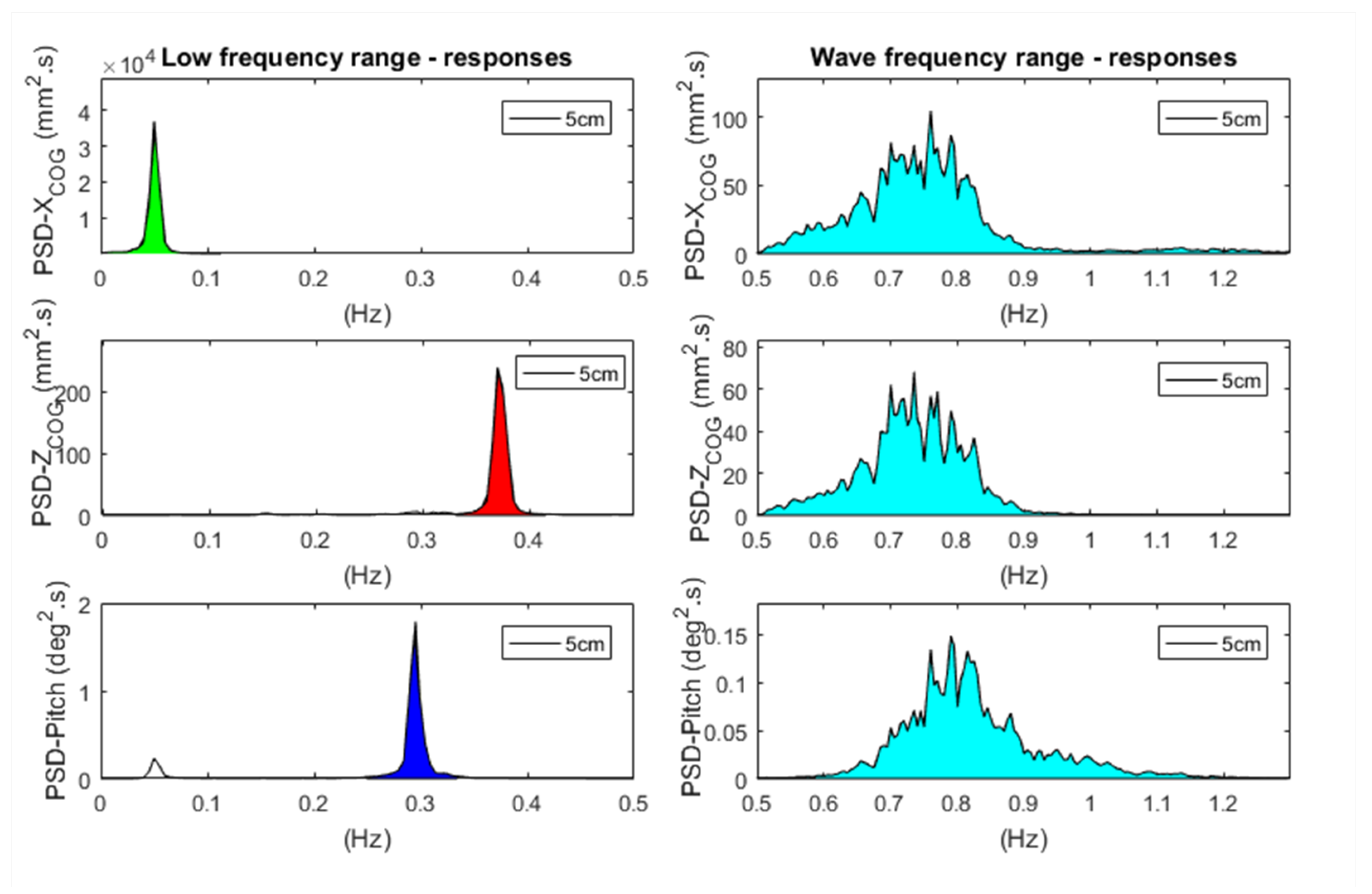
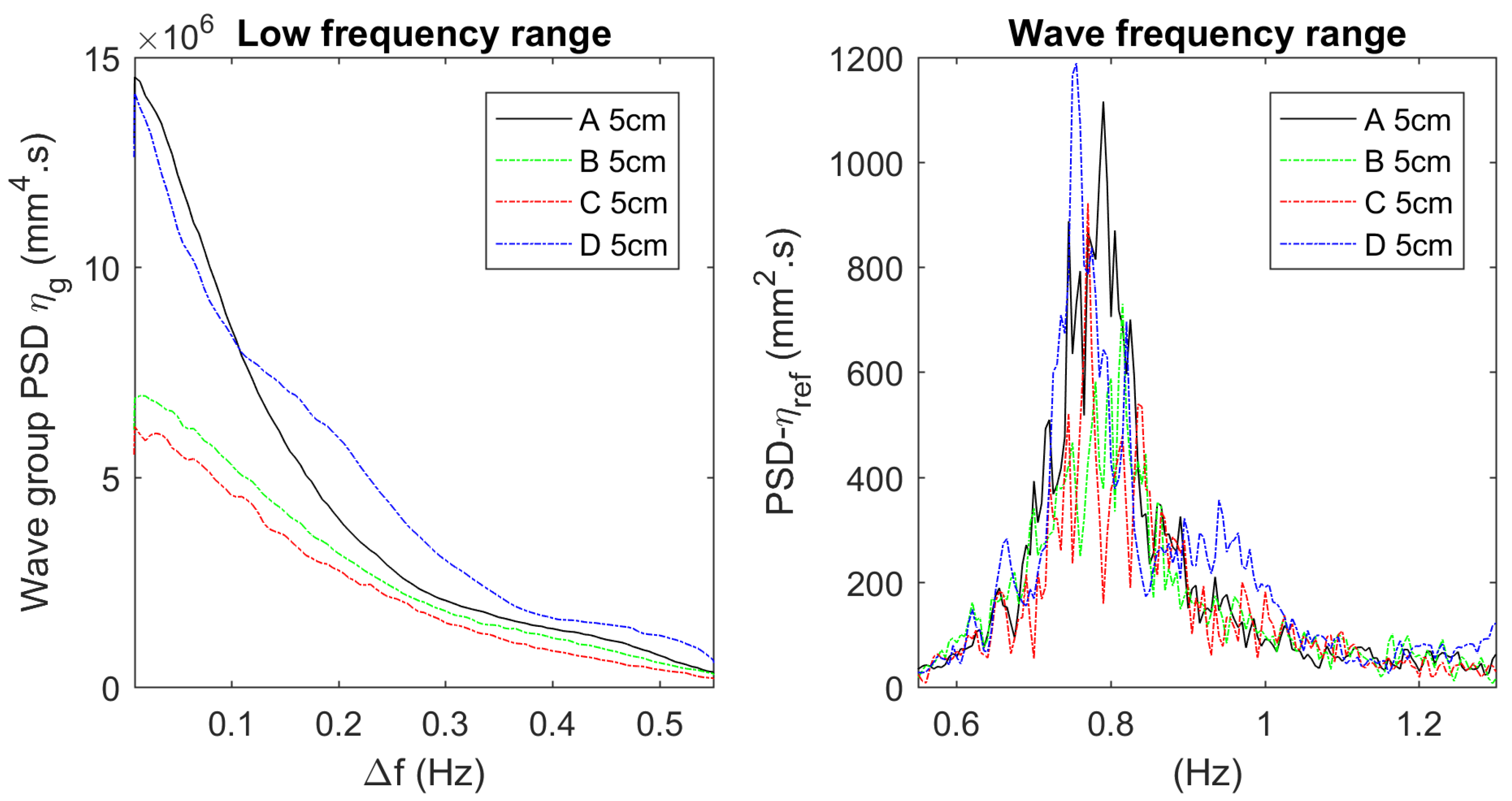
3. Responses in Irregular Waves

Irregular waves are essential to test any fixed or floating structures. They are more representative of real sea waves than regular waves. Spread moored floating structures move not only at the periods of the waves but also at longer periods matching the natural periods of their horizontal Degrees of Freedom (DOFs) [8]. The reproduction of these slow horizontal excursions with large amplitudes is essential for the estimation of mooring loads. For floating offshore wind turbines (FOWTs), low frequency motions in pitch and roll are important too because these motions interfere the most with the apparent wind velocity experienced through the rotor of the wind turbine. Accounting for the low frequency motion responses of a FOWT to waves is central in the design of an offshore wind turbine controller [9,10]. Therefore, the ideal analysis for a round robin test campaign should include the comparison of the wave frequency motions (i.e., the frequency range of target wave spectrum, hereafter referred to as WF) as well as the low frequency motions of the FOWT.
The test plan developed by Ifremer included irregular wave tests with and without wind thrust (see Table 2). Table 3 records the nature of the responses that can be expected per motion DOF for each JONSWAP wave, i.e., low frequency (LF) or wave frequency (WF). It also gives the range of frequencies which has been used to distinguish the wave frequency (WF: [ f 1 , f 2 ] (Hz)) from the low frequency range (LF: f < f 1 (Hz)). Gueydon et al. [7] discuss how each of these waves are likely to excite the model based on their power spectral densities and the associated group power spectral contents (see Table 3).

4. Metrics

Analysis of the round robin test results presented by [7] show that RAOs are suitable for studying the responses of the system in the wave frequency range. However, comparing the RAOs from multiple sources can quickly become difficult when multiple differences are observed. Moreover, RAOs shed light only on the wave frequency range. The main assumption behind the use of RAOs is the linearity of the response to wave height. Using a single value per test condition rather than the series of values making a RAO curve is preferable as it makes the comparison between basins easier to read. An approach based on metrics helps to efficiently assess the overall resemblance and dissimilarity between results from multiple basins. In this research, wherever possible, a single metric is prioritised over more detailed analysis results. This is done with the objective of limiting the analytical interpretation to its strict minimum and to support a more heuristic comparison process.
In this section, the zeroth and second moments of the wave frequency spectrum [11] are rewritten on the limited range of frequencies [ f 1 , f 2 ] (Table 3) which is used for the analysis of the irregular wave tests:
m 0 = f 1 f 2 S η d f ,
m 2 = f 1 f 2 f 2 · S η d f ,
where S η is the spectrum of the wave elevation, [ f 1 , f 2 ] is the wave frequency range and f the frequency (in Hz). Figure 1 shows the theoretical spectrum for the JONSWAP wave with T p = 1.29 s. The area shaded in cyan represents the area considered for the calculation of m 0 . For narrow banded spectra (like JONSWAP), H s is related to m 0 by the relation
H s = 4 m 0 .
Note that H s of Equation (3) underestimates the actual significant wave height as m 0 is integrated on a limited range of frequencies in Equation (1). Aside from m 0 and H s , another metric is introduced to provide us with an estimated value of the realised peak period, T p [12], calculated from:
T p = f 1 f 2 S η 4 d f f 1 f 2 f · S η 4 d f .
Equations (1) and (2) are used to obtain an estimate of the zero-up crossing period of the irregular wave:
T 2 = m 0 m 2 .
An estimate of the wave steepness S s [12] can be deduced from H s and T 2 by
S s = 2 π H s g T 2 2
where g is the gravity constant. Calculating the integral of every response power spectral density (PSD) or spectral energy distribution over the investigated wave frequency range gives us a quantity that should depend linearly on m 0 if the system is linear. These integrals for surge, heave, and pitch are shaded in cyan in the right hand plots of Figure 2. Therefore, the ratio of the area of the signal’s PSD and the wave PSD calculated over the wave frequency range provides us with a single value which represents how the wave power and the signal power are related. Under the assumption of a linear response, this ratio should remain identical when a system responds to the same spectral shape (e.g., JONSWAP with T p = 1.29 s and γ = 3.3 ) but different H s .
The metric used to examine the response of the system in the wave frequency range, M W F is calculated from
M W F = f 1 f 2 S s i g n a l d f m 0 ,
where S s i g n a l is the PSD of the signal.
Semi-submersible platforms are prone to second order motions. This has been observed and well documented for offshore oil and gas structures [13] and semi-submersible foundations for FOWTs [14]. The link between second-order wave loading and motion responses outside the horizontal plane (e.g., pitch in head waves) has been demonstrated for the OC4 semi-submersible FOWT [15]. By nature, second-order loads are smaller than first-order loads. Their manifestation in the motions is purely coincidental and triggered by resonance. That explains why the low-frequency response comprises isolated peaks lying around the eigen frequencies f e of the system (see left hand plots in Figure 2). Out of the seven spectra shown in Table 2 (see also Figure 10 in [7]), five (those with T p = 1.81 s and T p = 2.58 s) are sufficiently broad to excite the system at the pitch or even heave natural period with first-order wave loads. Only the JONSWAP spectra with T p = 1.29 s do not overlap with the low frequencies (the eigen frequencies f e for surge, heave, and pitch are shown with arrows in Figure 1). Therefore, the JONSWAP T p = 1.29 s wave tests are in theory adapted to look for low frequency responses which are exclusively the effect of the higher order wave loads. It is difficult in practise to exclude the presence of long parasite waves in the basin outside the range of the target wave spectrum. Nevertheless, the existence of low frequency responses for surge, heave, and pitch in results of all tests done in all facilities reinforces the theory that these responses are due to the second order wave loads and not artifacts of a specific basin. Due to the higher order nature of the low frequency responses, any difference in wave excitation has an even bigger impact on the difference in the levels of excitation in surge, heave, and pitch. That makes it hard to comment on the level of the low frequency responses. Nevertheless, the presence and the location of these resonance peaks can be estimated by a metric similar to the one used to estimate the peak period of the waves. This new metric is called T r as it represents the period of the resonance response and is given by:
T r = f e δ f f e + δ f S s i g n a l 4 d f f e δ f f e + δ f f · S s i g n a l 4 d f .
where S s i g n a l is the PSD of the signal, f e is its main resonance frequency, and Δ f is a frequency band around f e that covers the peak shaped resonance response of the signal.
The reporting of the low frequency responses will be limited to these metrics (for surge, heave, and pitch) in this article. In relation with the layout of the test set-up and the tested conditions (i.e., head waves and head wind) (as described in [7]), these metrics are not presented for other motions than surge, heave, and pitch. As an example, the comparisons of the motion responses and tension responses for JONSWAP T p = 1.29 s and H s = 5 cm are developed using these metrics in the next section. These metrics consist of:
1.
H s calculated over the wave frequency range divided by the targeted H s value.
2.
T p calculated over the wave frequency range divided by the targeted T p value.
3.
S s calculated over the wave frequency range divided by the targeted S s value.
4.
M W F 
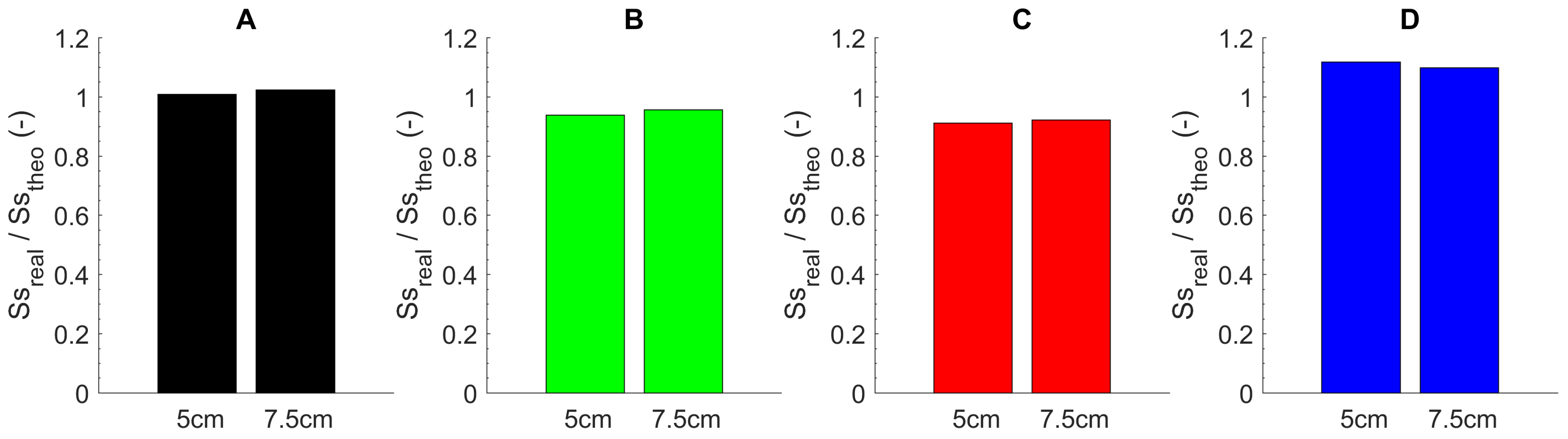
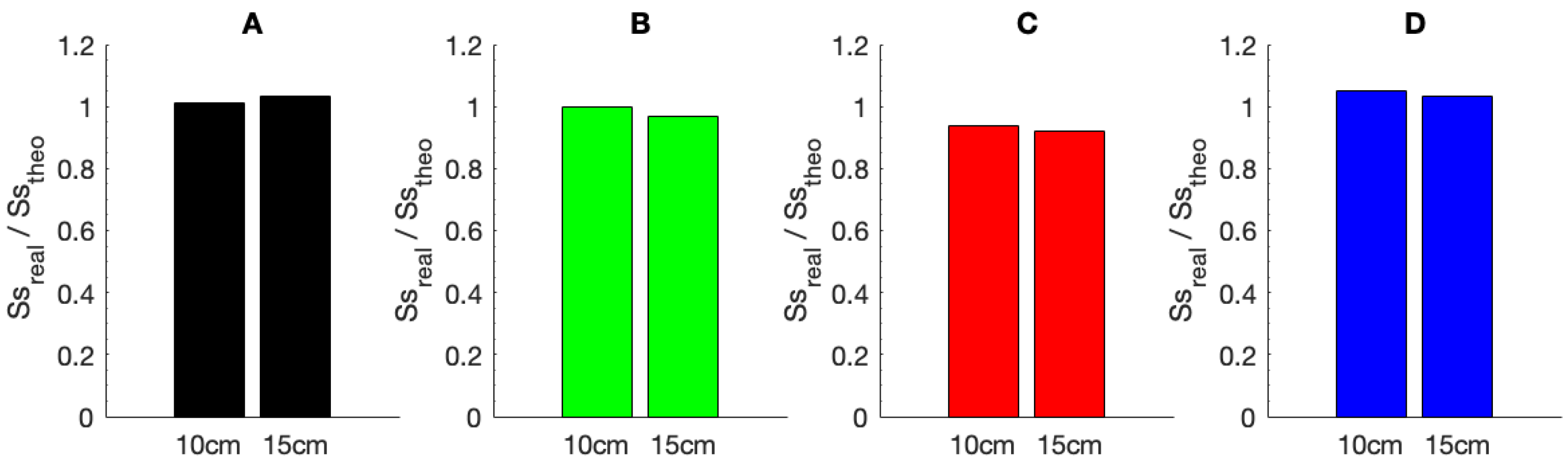
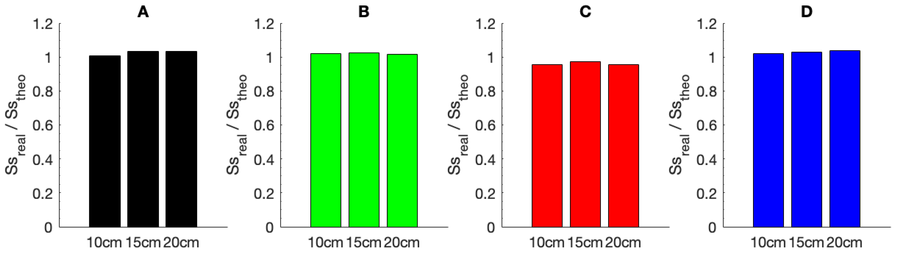
, the square root of integral of a response over the wave frequency range divided by m 0 .
5.
T r 
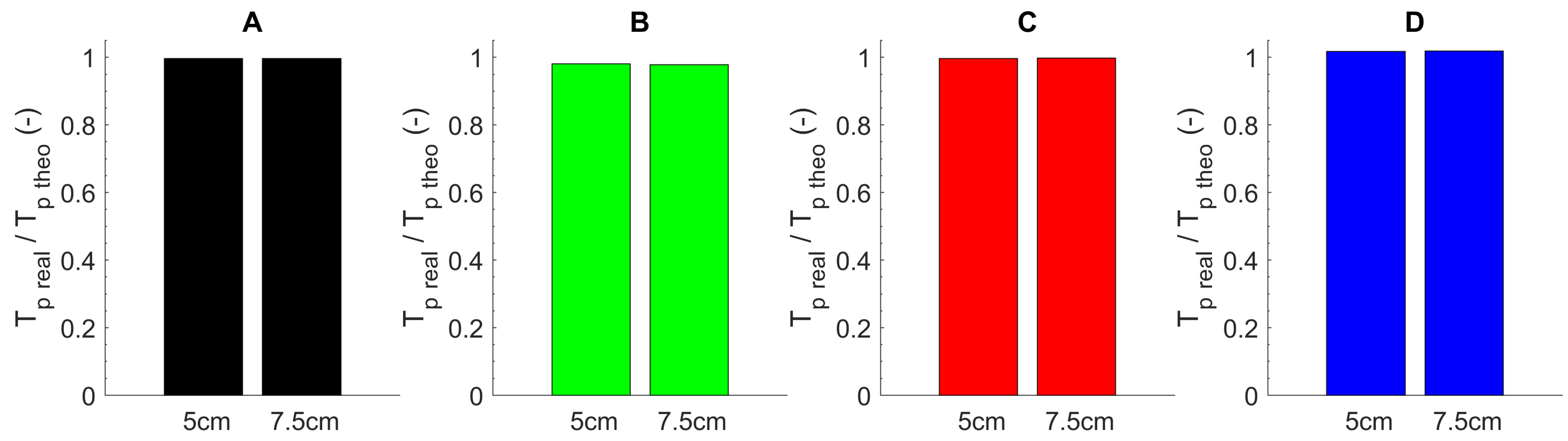
, the period associated with the resonance peak of the response.

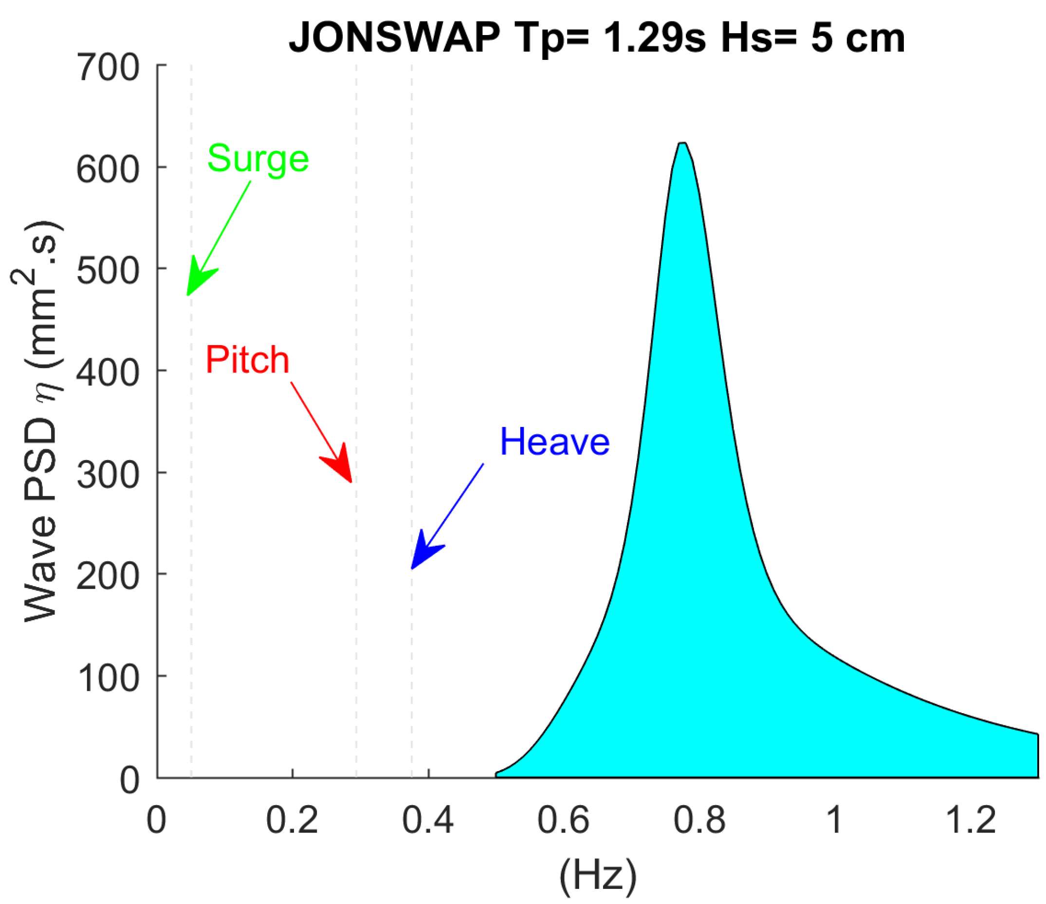
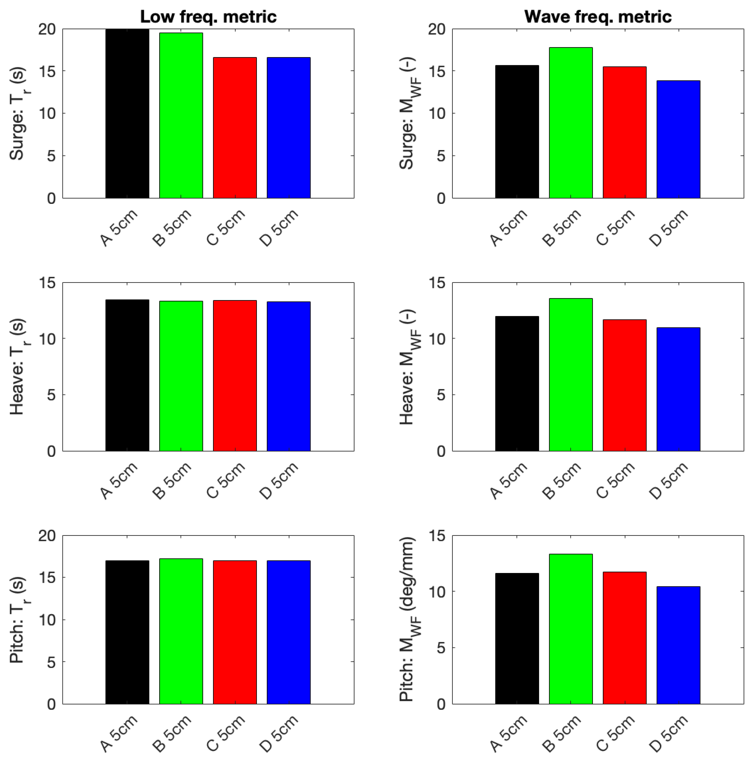
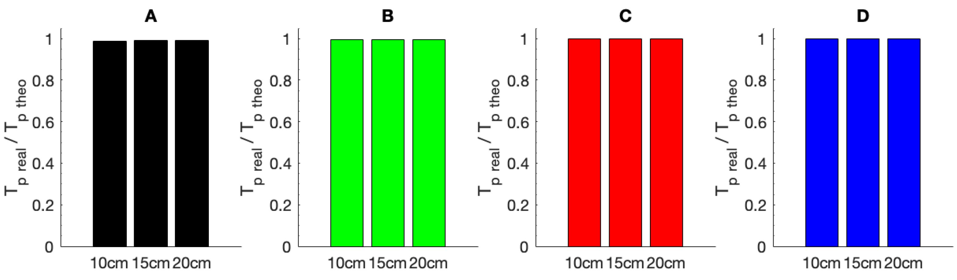
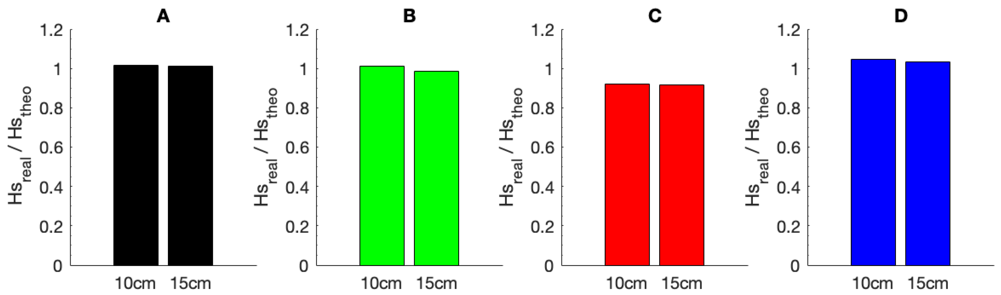
Application of the Metrics to Tests with JONSWAP T p = 1.29 s H s = 5 cm

During the round robin tests, all basins attempted to generate a wave as close as possible to the JONSWAP T p = 1.29 s theoretical wave. It can be seen from the realised wave spectra shown in the right plot of Figure 3 that variations are significant. These variations are more noticeable in the calculated H s (Figure 4 and Figure 5) and significant steepness S s (Figure 6) than in the peak period T p (Figure 7). On the x axis of the left hand plot of Figure 3, Δ f is the difference frequency that is used to calculate the wave group spectrum (see [7] for a detailed explanation). Differences between the wave group spectra of all facilities are even larger due to quadratic nature of this spectrum. Despite these differences, the regions of the frequency axes that contain significant level of wave forcing are the same. This is valid for the wave frequency range and the low frequency range with some nuances.
As seen in [7], even if all basins share the same global shapes for all RAOs, there are still numerous deviations between facilities. It is difficult to establish which differences are more important than others and should be commented on. The comparison of the metrics gives a global picture of the variations between the results from all basins that is easier to interpret. For instance, the top left graphic in Figure 8 shows that the resonant peak in surge is not located precisely at the same frequency for all facilities. The surge eigen frequency differs for D. This is in line with the discrepancy in surge stiffness and its impact on the natural period reported in [7]. For C, the shift of the surge resonance peak is more surprising and will be discussed later. The metric T r is able to catch these differences. The good agreement of T r for heave and pitch between all basins (middle and bottom left plots) confirms the stability of the resonance frequencies for these modes across all test set-ups. In the hypothesis of purely linear motions, M W F shown on the right column of Figure 8 should be identical for all basins; however, clearly it is not identical. This metric makes it possible to identify how much the response to waves varies between facilities. Basin B gives the biggest motions and D the smallest. The difference is the most significant for pitch (24%). The differences between facilities are bigger for the tension metrics than for the motion metrics (up to 47% for the port (PS) and starboard (SB) mooring lines, Figure 9). Although, the comparison of metrics is much easier to read than PSDs or RAOs; the metrics inevitably lose the level of detail of the RAO plots (see [7]).

5. Results

The results of the tests in irregular waves carried out during the five distinct campaigns (A, B, C, D, and E) are presented and compared in this section. This includes the tests without and with thrust. The metrics introduced in the previous section are implemented here. For most of the tests, only the main motion metrics are displayed for brevity.

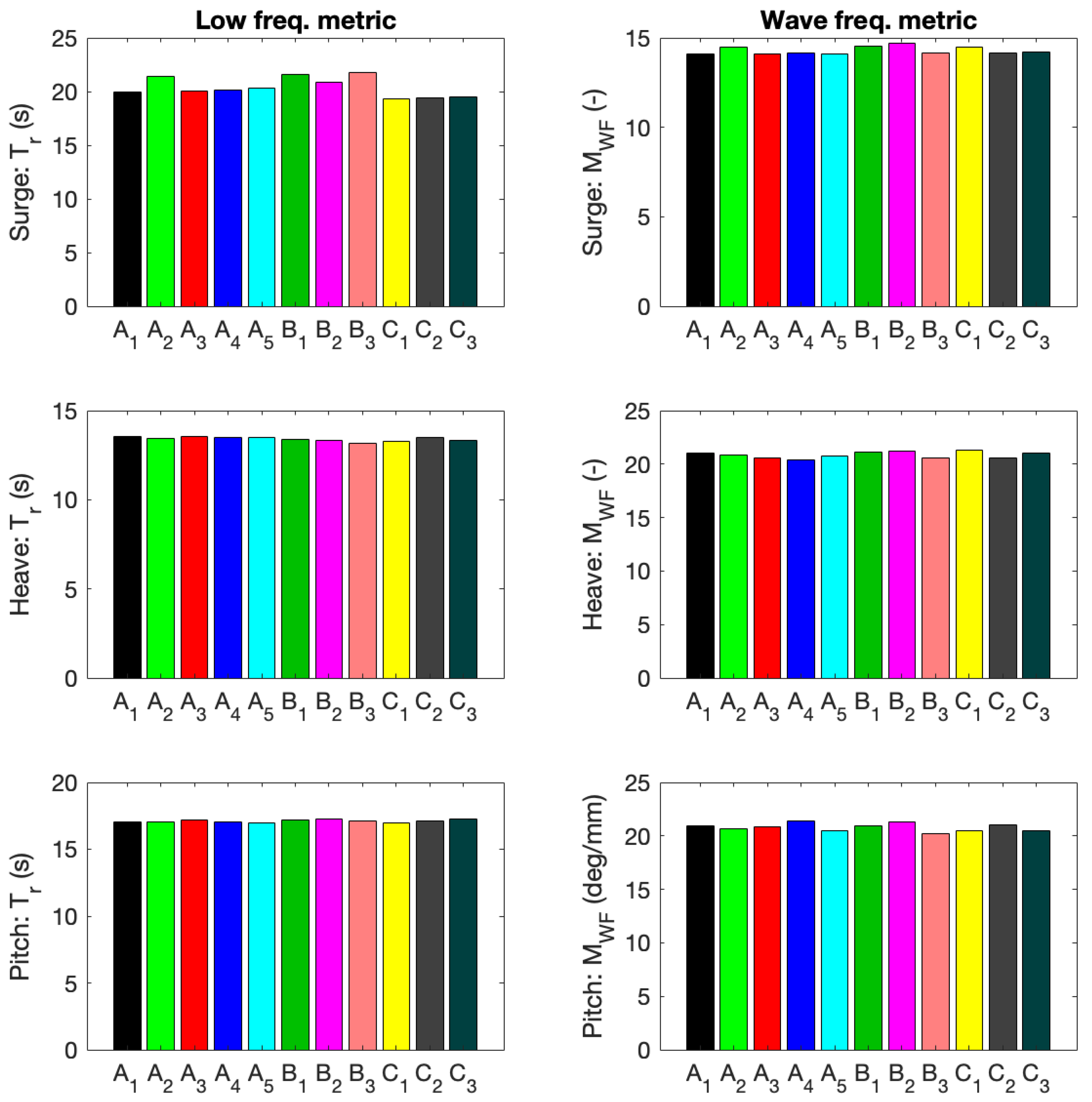
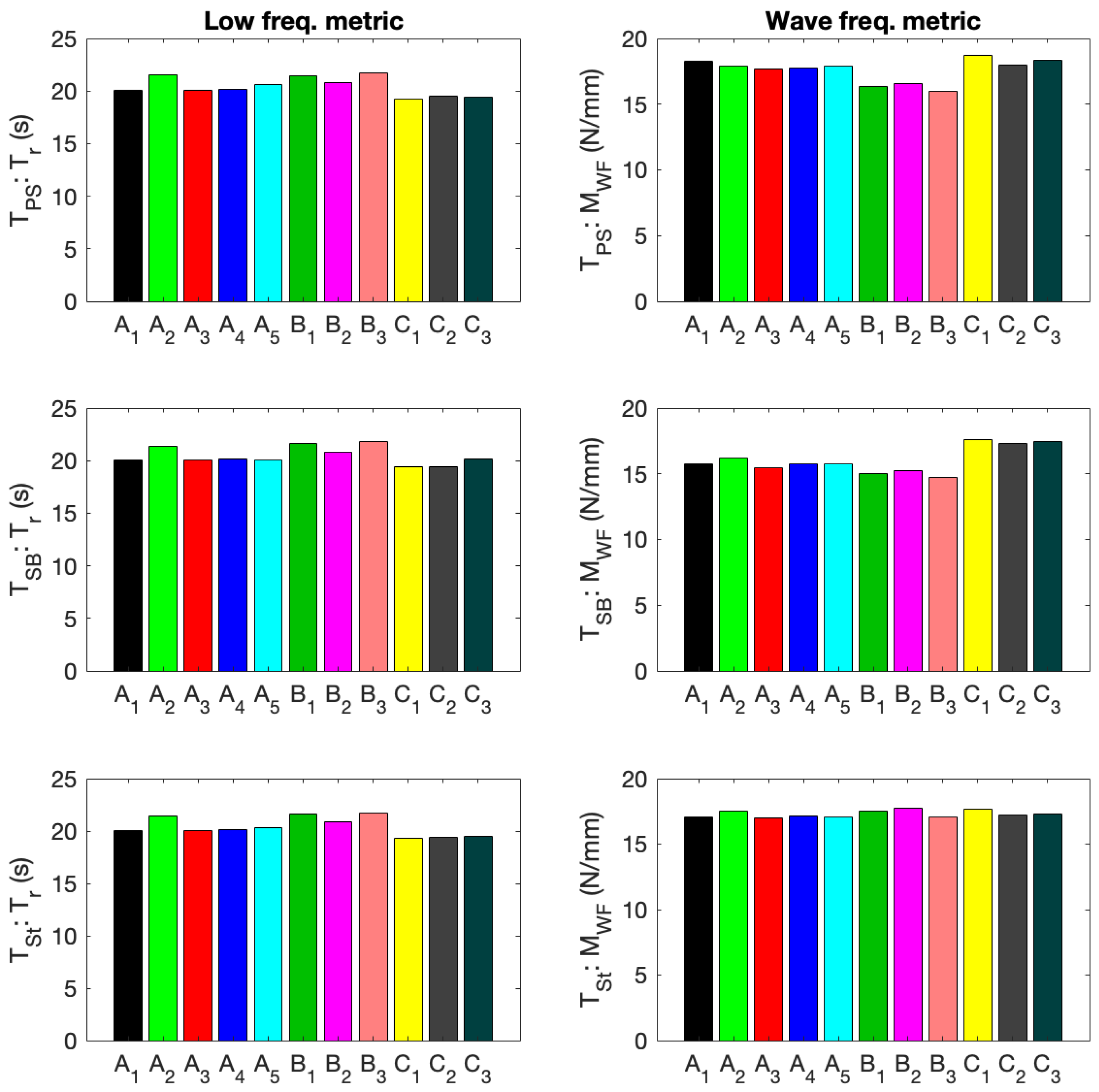
5.1. Effect of Wave Seed on Responses
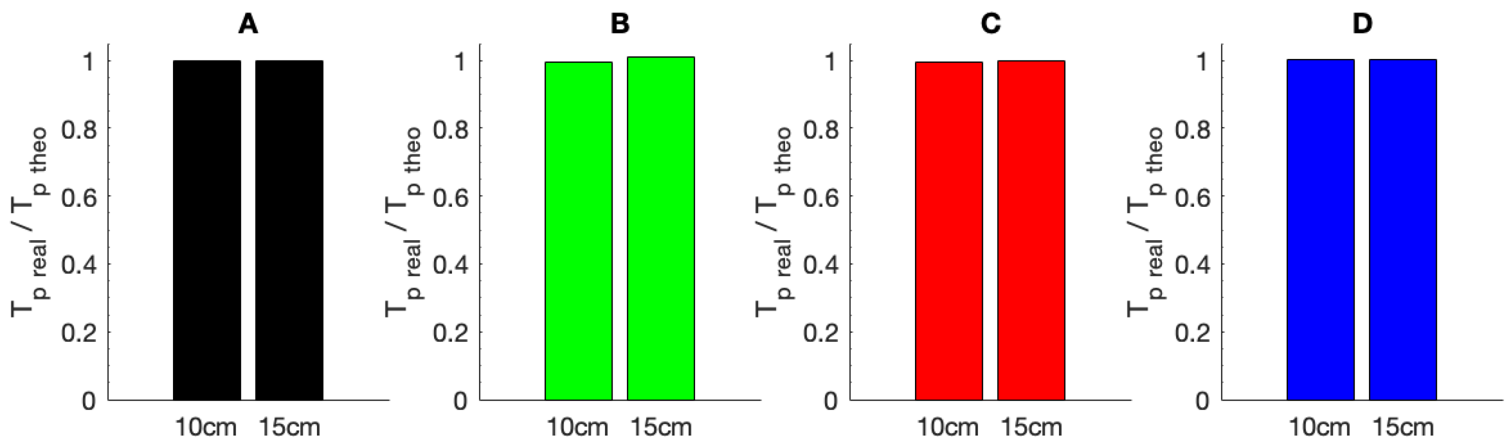
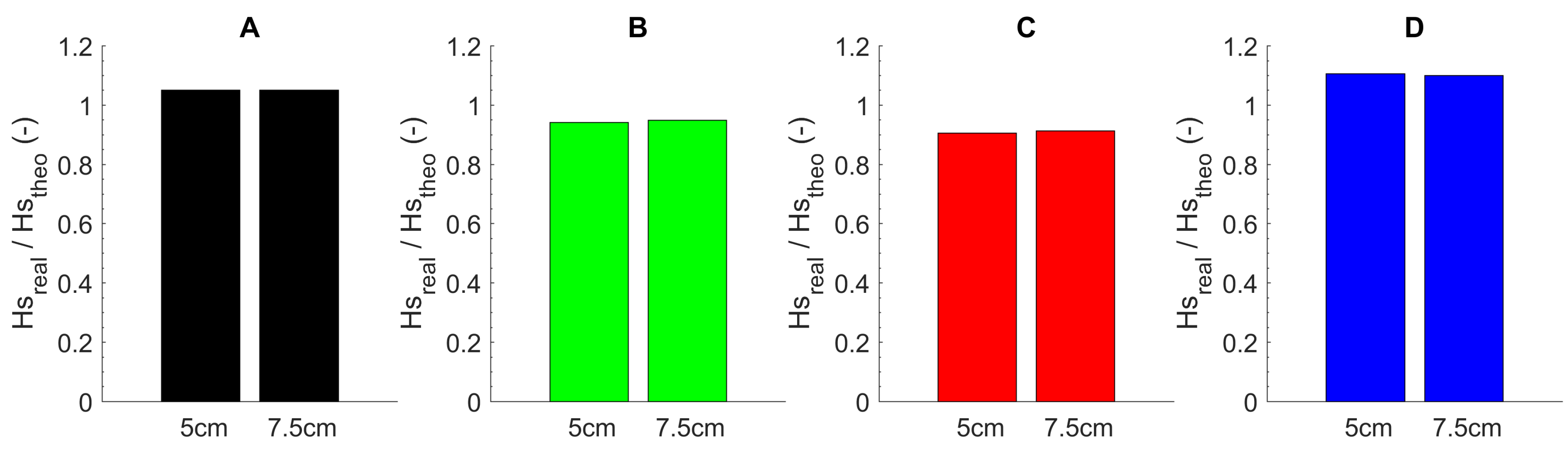
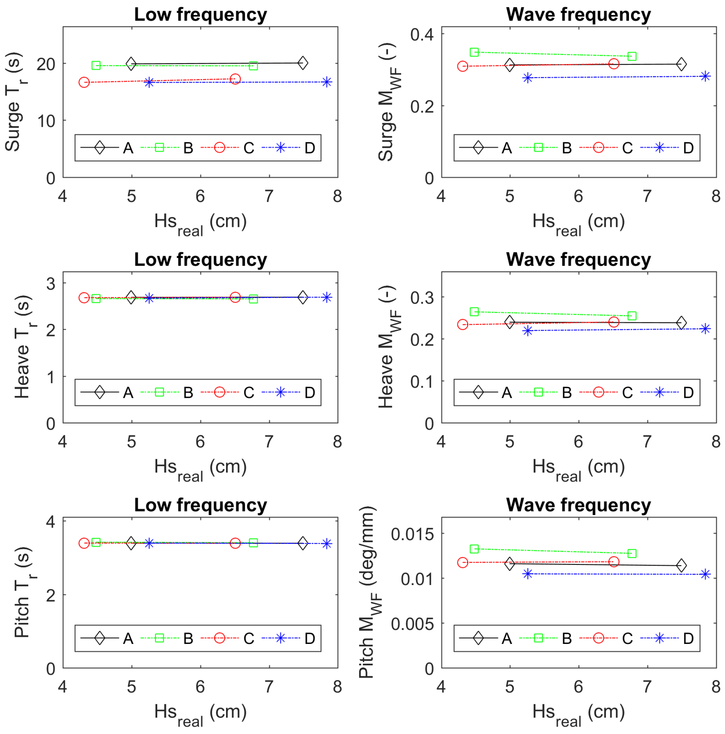
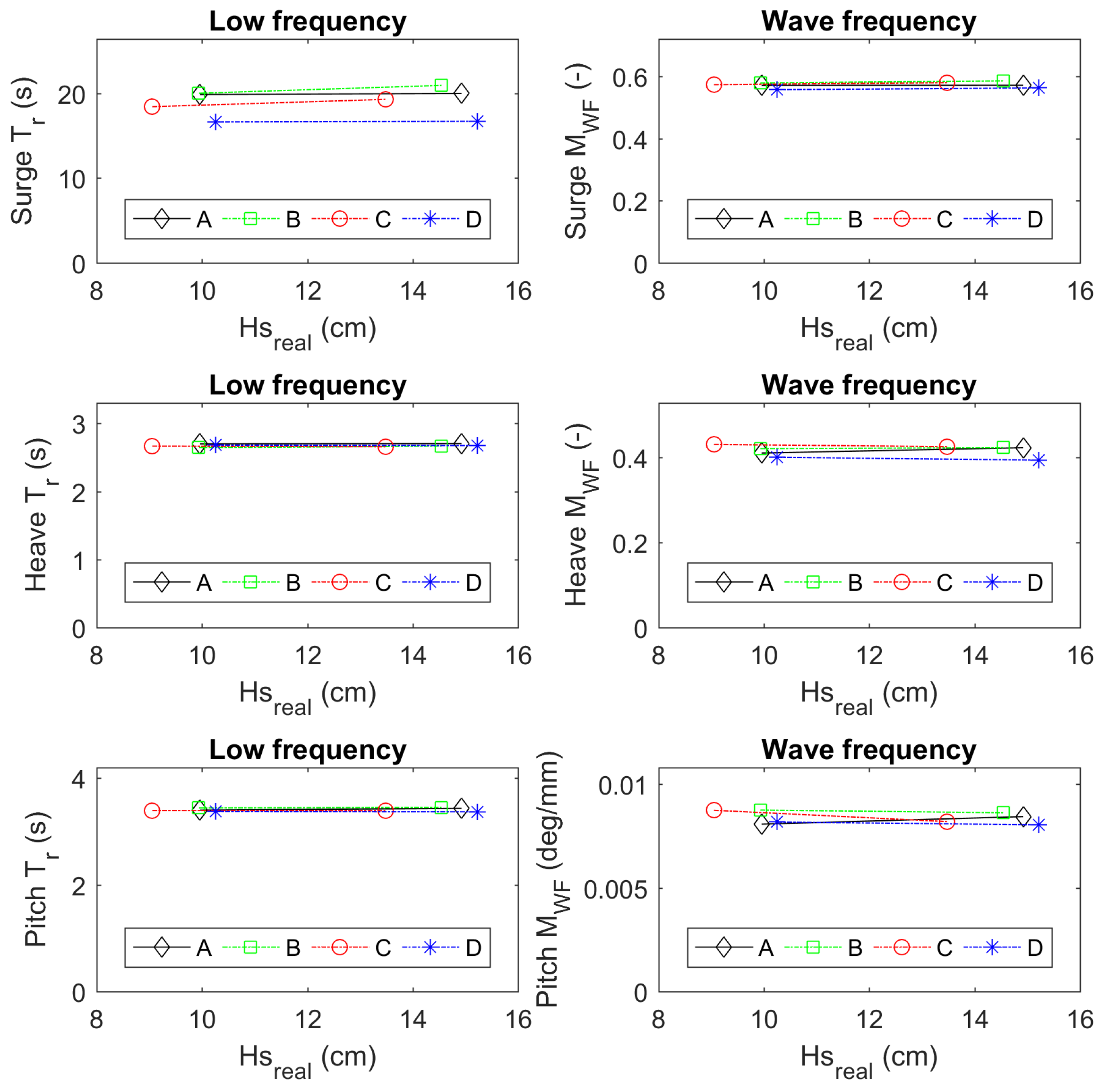
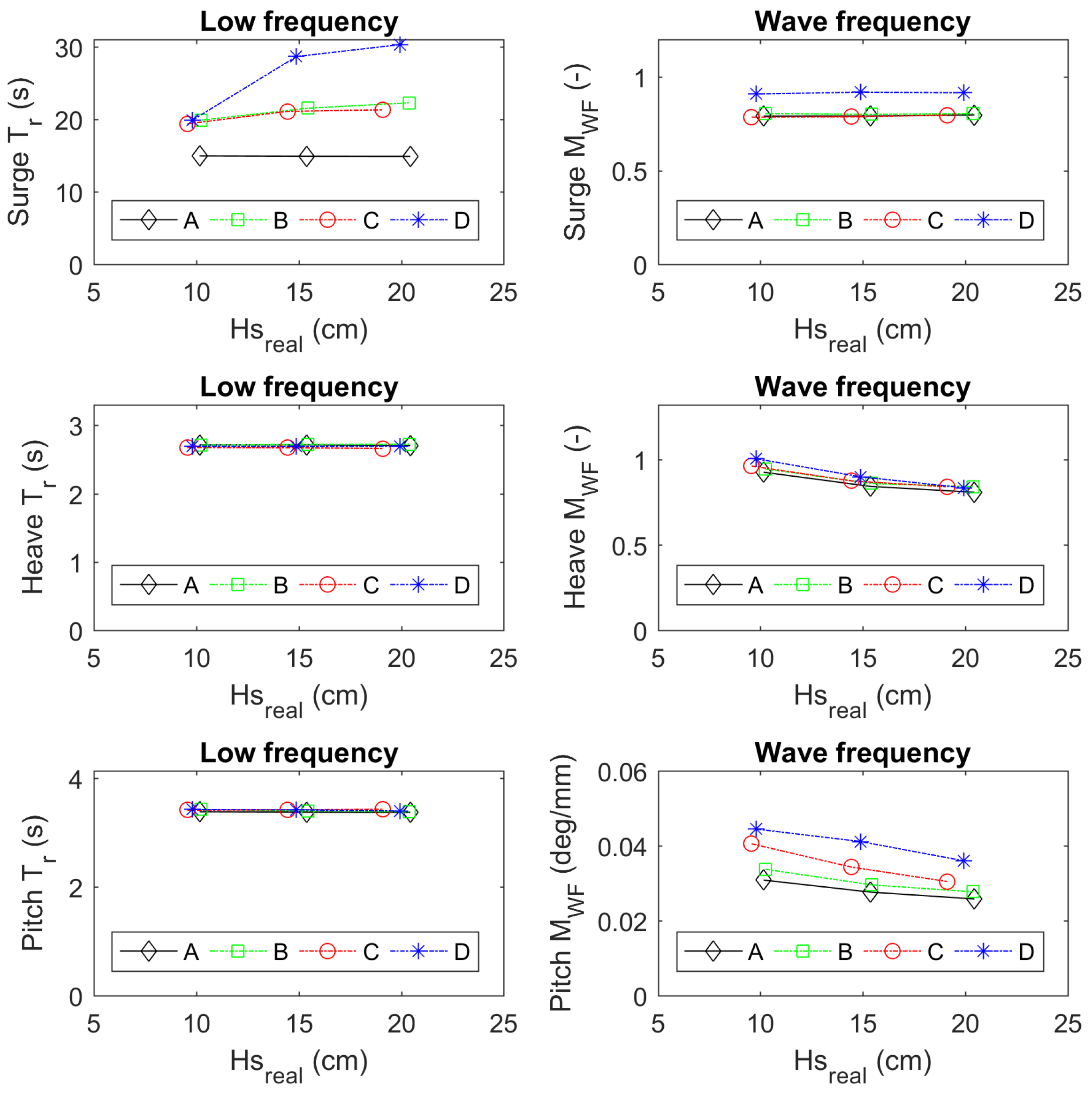
Similarly to [7], the JONSWAP waves with T p = 1.81 s and H s = 15 cm generated with different seeds are used to study the effect of randomness on the results. These tests were done in Basins A, B, and C with the same target spectrum but distinct seeds.
The estimates of the resonance periods for surge, heave, and pitch are displayed in a bar-plot (left column of Figure 10). The index given in the subscripts of A, B, and C correspond to repeat waves generated with a unique seed. The metrics M W F are given in the right column for surge, heave, and pitch. Figure 11 shows the same graphics for the mooring line tensions. The three signals processed in this graphic are: T P S , the tension in the line at portside; T S B , the tension in the line at starboard; and T S t , the tension in the stern line. In general, all tests independent of facility and seed give globally similar results for these metrics. Nevertheless, there are differences between facilities and also within the same basin for distinct seeds.
The deviations between results of tests in waves with different seeds per basin are presented in Table 4. The last column of Table 4 contains the deviations when results from the three basins are considered together. Note that this last column is given as an indication and should be considered with caution as the number of seeds and the duration of the tests are different for A, B, and C. As reported in [7], H s varies a lot more than T p with the seed. Among the motions, the differences are larger for the surge T r and the pitch M W F . The deviations of T r and M W F are bigger for the tensions than for the motions. The deviations in the metrics between basins are larger than those caused by different seeds within a facility, as was observed with the RAOs presented in [7].

5.2. Effect of H s on the Metrics

Looking at the realised irregular waves for all wave heights in all basins, it is remarkable that the peak periods ( T p ) are always very close to the target theoretical value (Figure 7, Figure 12 and Figure 13). Whereas there are significant deviations between the realised significant wave heights ( H s ) and the target values (Figure 5, Figure 14, and Figure 15). Furthermore, the spread between facilities is significant, with some below the target H s while others are over it. The same discrepancies were noticed for the significant steepness ( S s in Figure 6, Figure 16, and Figure 17). This justifies the strategy of checking if trends between the response metrics in different basins are equivalent rather than comparing the metrics directly. The metrics have been calculated for the different values of H s . They are displayed for each JONSWAP wave and all basins in Figure 18, Figure 19 and Figure 20.
The resonance peak periods ( T r ) were determined based on Equation (8) for all response signals. It was found that for heave, the values of all facilities were grouped and stable with increasing wave heights. This was also true for pitch. For heave and pitch, the values of T r are similar to the natural periods derived from the decay tests in still water without thrust, as presented by [7]. For surge, T r is more erratic and often not aligned with the surge natural period of the decay tests (which are reported in [7]). As expected, the deviation reported in the surge natural period for basin D caused by a stiffer mooring system was still present. However, T r also varies between different waves ( T p and H s ) in the same basin. These variations are very important for the longest irregular wave (JONSWAP T p = 2.58 s). As this was observed with the results of all facilities, it is most likely inherent to the tested system. A closer look at the cases with the largest variations revealed that several resonance peaks are located close to each other rather than a single resonance peak. The second largest peak often appears to coincide with the sway resonance frequency even when the sway motions are much smaller than the surge motion. This suggests that a coupling between surge and sway can sometimes arise and disturb the surge motion. Although this cannot be easily proved, the power cable could well be responsible for this disturbance. The presence of oblique reflection can also cause this disruption. In heave and pitch, T r stays at the same level independently of H s for all facilities. For surge, T r exhibits important variations with no apparent trend with regard to H s .
For all irregular waves, the values of M W F for surge do not vary significantly with the wave height. The trend is stable for all facilities (i.e., the lines on the plots are generally horizontal). On the other hand, the differences between basins are sometimes large, i.e., the vertical distance between the lines (e.g., for the shortest wave (Figure 18) and the longest wave (Figure 20)). For heave, M W F is stable when H s increases for two of the three irregular waves ( T p = 1.29 s and T p = 1.81 s (Figure 18 and Figure 19)) whereas it drops for T p = 2.58 s (Figure 20). This drop can be associated with the decrease of the heave resonance peak observed in the plot of the heave RAO for increasing H s [7]. A significant drop is also observed for pitch when H s grows for the longest wave. This decrease also reflects the decrease of the resonance peak of the pitch RAO with increasing H s as observed by [7].
Most importantly, the metrics applied to surge, heave, and pitch are showing the same trends with regard to the variation of H s for all facilities.

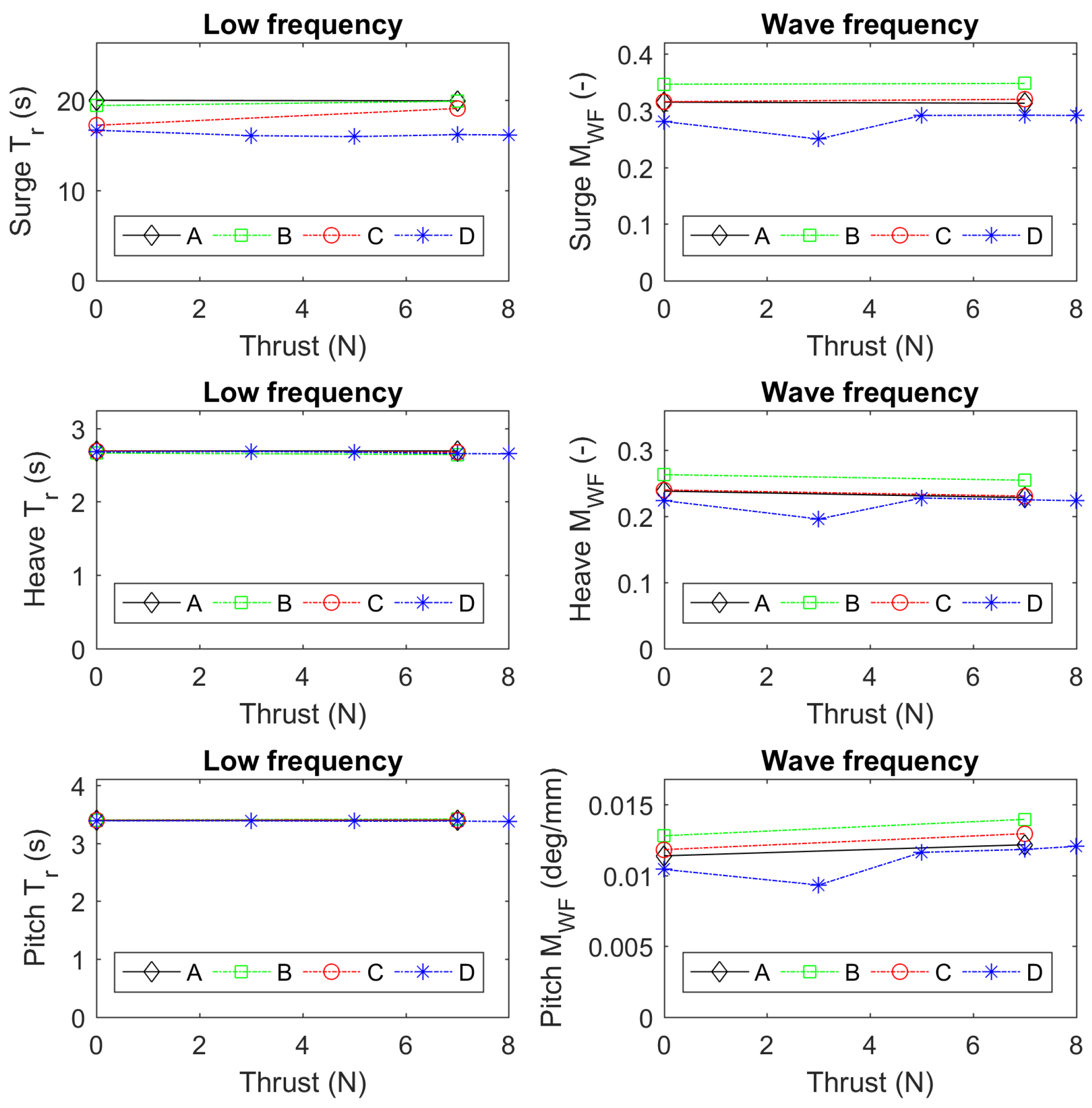
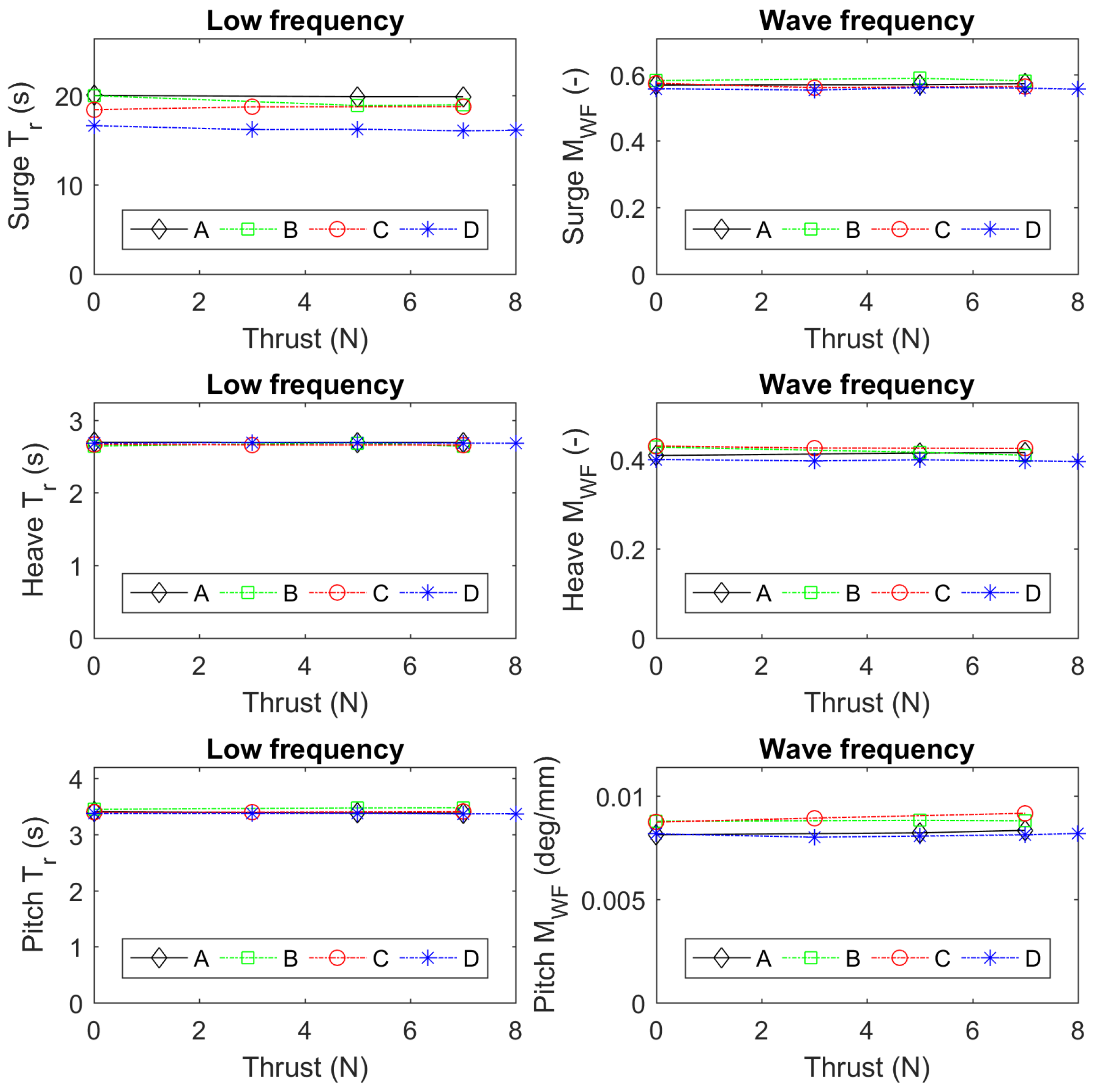
5.3. Effect of Thrust on Responses in JONSWAP Waves with T p = 1.29 s and T p = 1.81 s

The variations in the resonance peak period for surge, heave, and pitch are small for all facilities. T r is very stable for heave and pitch for all basins whereas T r often varies for surge in different ways for distinct basins. The resonance peak in surge for C appears to vary more than for the other basins. No global trend can be extracted for the variations of the resonance peak periods that can be attributed to the increase of the thrust (Figure 21, Figure 22, Figure 23 and Figure 24). Except for a few outliers, the surge M W F metric is mostly stable. For these waves, no response is greatly affected by the different levels of thrust. This is true for surge, heave, and pitch. The same can be said for the mooring line tensions (not shown).

5.4. Effect of Thrust on Responses in JONSWAP Waves with T p = 2.58 s

For the waves whose spectra cover the resonance responses in heave and pitch (i.e., T p = 2.58 s), the picture is very different from the JONSWAP waves discussed in the previous section. The thrust variation included all possible steps that the propeller system could provide (0N, 3N, 5N, 7N, and 8N); however, these tests were performed at only one facility (D). While the surge and heave M W F metrics decrease slightly with increasing thrust, the pitch metric decreases more noticeably under the effect of the thrust (Figure 25). This evolution of the M W F metric is consistent with the evolution of the RAOs documented in [7]. These reductions can directly be related to the drop observed in the resonance peaks for heave and pitch and reported in [7]. The study of the metrics confirms that the effect of the thrust is most significant on the heave and pitch for the longest wave. The observed decrease is more pronounced for pitch than for heave. The resonance peak in surge is impacted by the thrust. However, the variations of the surge T r under thrust are different between the three levels of H s (10 cm, 15 cm, and 20 cm) that were tested. It is therefore not possible to extract a trend describing how T r for surge varies with the thrust. Moreover, these variations are much smaller than the changes in T r observed between H s = 10 cm and H s = 15 cm. T r for heave and pitch do not vary significantly with the level of thrust.

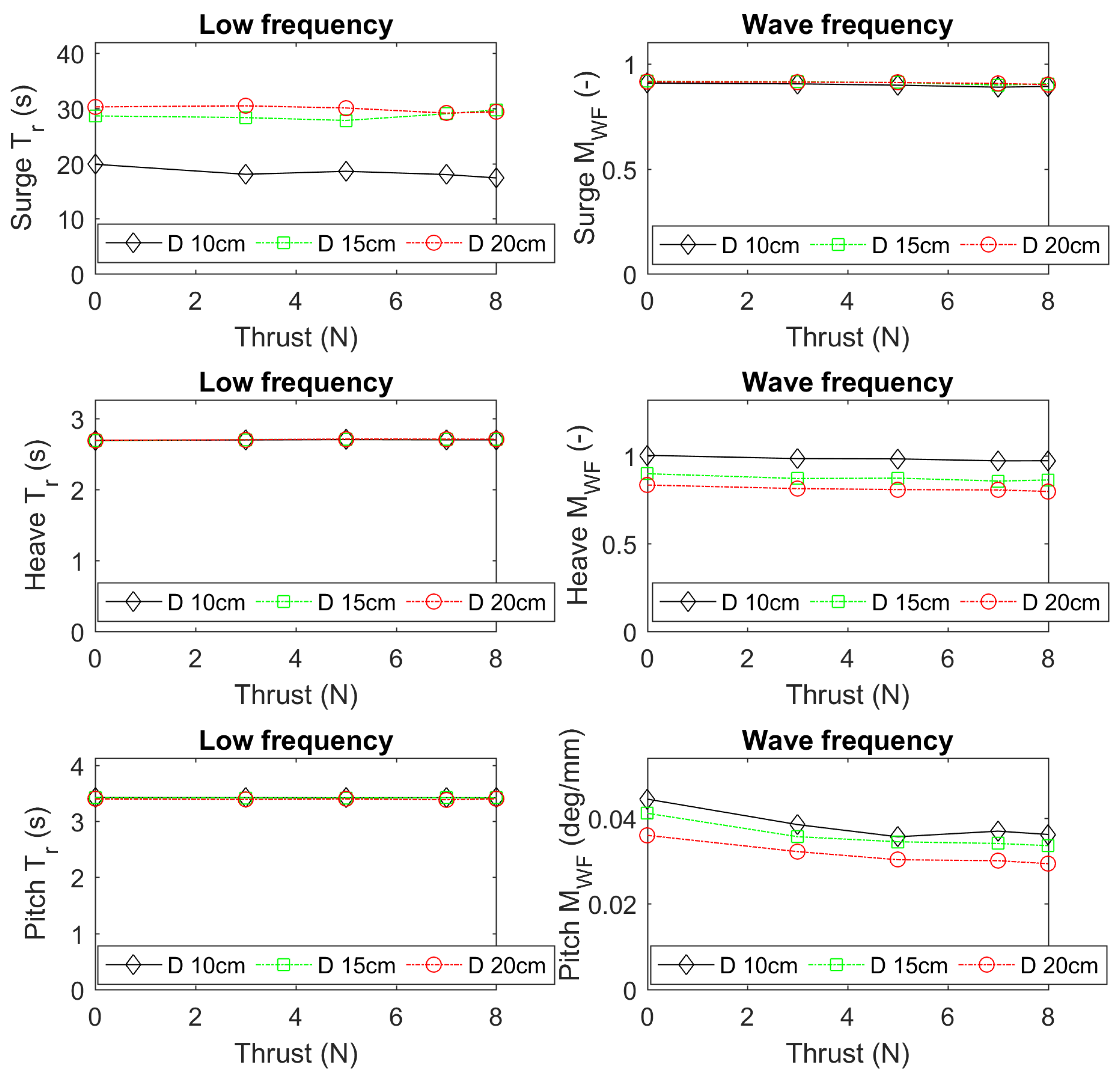
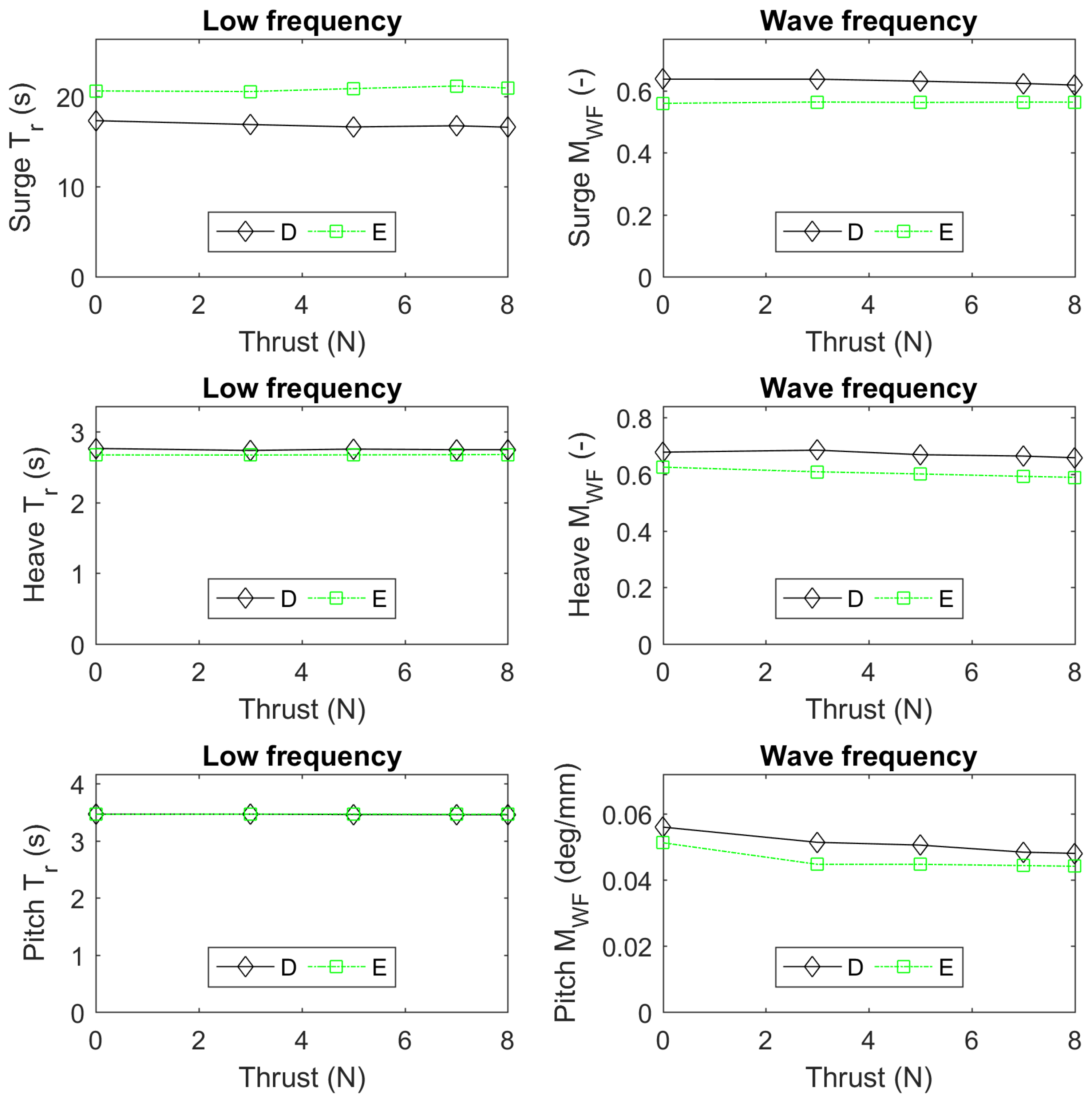
5.5. Effect of Thrust on Responses in the Pink-Noise Waves

The spectra of the Pink-Noise waves cover the resonance responses in heave and pitch. These waves were run in combination with thrust in two facilities (D and E) for the same five steps as for JONSWAP with T p = 2.58 s. For surge, the impact of the thrust on the metrics T r and M W F was mild but opposite in D and E (Figure 26). As a consequence, no trend could be extracted for surge. For heave and pitch, the response periods appear to be stable when the thrust varies. M W F is decreasing in pitch. This confirms that the thrust acts mainly on the pitch by lowering its response. We know from the study of the RAOs in [7] that this decrease primarily occurs around the pitch resonance. For the tension, the trends of D and E are not the same but it can be said in both cases that the effect of the thrust on the surge T r and surge M W F are mild (not shown).
In summary, the thrust has the most significant impact on the pitch response and causes a decrease of the pitch resonance peak [7]. Therefore, this impact is mostly visible for waves which are long enough to properly excite the pitch period. Other effects in heave and pitch are mild. Although the surge metrics are often not significantly affected by the thrust, they sometimes seem to give chaotic results as they vary with the wave height, the thrust, and the facility. Except for surge, the trends that T r and M W F follow are globally identical for the majority of the testing campaigns.

6. Discussion

6.1. Advantages of Using Metrics

The evolution of the metrics with the significant wave height has been compared across all basins. Some common trends have been identified from this exercise. For heave and pitch, the resonance response periods ( T r ) were stable for all wave heights. For surge, the resonance period was erratic and often differed from the surge natural period of the decay tests. This point deserves more attention than what it has been given in the present study and could be the object of further work. M W F was designed as the main metric addressing the linear response of the system in the wave frequency range. Its evolution with H s has revealed that the system stops behaving linearly for long waves. Heave and pitch responded non-linearly to long irregular waves. These metrics for heave and pitch decreased with the wave height for all facilities.
For tests with increasing level of thrust, the trends observed in the evolution of the metrics were the same in the four basins. The effects of the thrust on the surge and heave M W F metrics were mild for all wave conditions. The impact of the thrust was the largest on the pitch metric M W F for the JONSWAP wave with T p = 2.58 s. The surge response peak period T r is also impacted by the different levels of thrust. However, no logical trend could be identified for these variations. It seemed to be more randomly affected by the different thrust levels. In addition, discrepancies between facilities for this metric were significant. The response peak periods for heave and pitch did not change with the thrust.
All these findings corroborate the findings of the study of the RAOs presented in [7]. The two global trends leading the response of the system, i.e., the wave height and the wind thrust, were more clearly apparent in the plots of the metric M W F than in the plots of RAOs. It has been shown that these metrics are powerful tools to find the trends common to several basins. The metrics can also easily support a quantitative comparison. The use of metrics allows for a heuristic comparison of results from distinct basins that cannot be easily compared directly as they are not obtained in identical conditions. The extraction of trends from a selection of metrics is an efficient way to overcome the impossibility of generating an identical wave in distinct facilities. Metrics can also serve the benchmarking of numerical simulations against model-tests [16].

6.2. Limitations of Metrics

A limited number of metrics were used for the comparison of the tests in different facilities and different conditions. Although these metrics are good indicators of the level of agreement between tests, they do not show all possible discrepancies. No efforts to quantify the difference in the amplitude of the responses over the low frequency range have been done due to the lack of a good metric for this purpose. In addition, the duration of the irregular wave tests was not equal in all basins and often shorter than the recommended three hours at prototype scale (i.e., 1394 s in the basins). This is a source of uncertainty that needs to be explored. Furthermore, some differences in the appearance of responses in low frequencies but outside the expected resonance peaks for surge, heave, and pitch have not been discussed. Further research is still necessary to obtain a clearer view on the agreement of the responses in the low frequency range. An analysis focused on the low frequency responses would require the introduction of new metrics that can overcome the disparity between wave amplitudes and spectral shapes achieved across all basins. It would also be preferable to have a better convergence between the realised waves in all facilities for any comparison focused on the low frequencies. The frequencies higher than the wave frequencies have been ignored because they are not deemed to be of importance for the response of a semi-submersible platform [15].

7. Conclusions

This paper promotes the use of metrics for the comparison of model-test results from distinct basins. A number of metrics have been introduced and applied for the analysis of round robin tests of a floating wind turbine in hydrodynamic basins. These metrics have been very helpful in extracting global trends. They have been used to assess how the responses vary with the wave height and the applied thrust. Aside from illustrating the good agreement between the results from all participating basins, the paper also looks for differences and elaborates on their causes. This investigation is based on a large part of the available test data (i.e. all irregular wave tests). The presentation of the results involves metrics that inevitably narrow the vision on specific aspects of interest to the authors. The main targeted aspect was the linearity of the responses of the system to the waves. There are undoubtedly many other ways to scrutinise these data and shed light on other relevant relations between the data and the characteristics of the basins for instance. One of the major outcomes of this round robin testing is the public availability of the data. This will make it possible for others to do their own investigation and build their own interpretation of similarities and dissimilarities between results from different facilities.

Author Contributions

Conceptualisation, S.G.; methodology, S.G.; formal analysis, S.G.; investigation, F.J., E.L., M.O., F.T., M.L.B., J.C., J.O., B.B., S.K., S.D. (Shinwoong Kim), S.D. (Sandy Day); data curation, E.L., M.L.B.; writing—original draft preparation, S.G.; writing—review and editing, F.J.; visualisation, S.G.; project administration, M.O., J.M.; funding acquisition, J.M.; supervision, J.M. All authors have read and agreed to the published version of the manuscript.

Funding

This research was funded by European Union’s Horizon 2020 research and innovation programme under grant agreement number 731084, project MaRINET2 (Marine Renewable Infrastructure Network for Enhancing Technologies 2).

Data Availability Statement

The data obtained during this test campaign will be made available on the MaRINET2 e-infrastructure. The data from the first test at UCC is available at [17].

Acknowledgments

UCC would like to acknowledge the contributions of Cian Desmond, Tom Walsh, and Christian van den Bosch to the round robin campaign.

Conflicts of Interest

The authors declare no conflict of interest.

Abbreviations

The following abbreviations are used in this manuscript:
CoGCentre of Gravity
DoFDegree of Freedom
FOWTFloating Offshore Wind Turbine
ITTCInternational Towing Tank Conference
JONSWAPJoint North Sea Wave Project
LFLow Frequency
MoIMoment of Inertia
OREOffshore Renewable Energy
PSDPower Spectral Density
RAOResponse Amplitude Operator
WFWave Frequency

Notes

1
www.marinet2.eu (accessed on 17 September 2021).
2
Register of ITTC guidelines is available at https://www.ittc.info/media/4251/register.pdf (accessed on 17 September 2021).

References

  1. Gueydon, S.; Bayati, I.; de Ridder, E.J. Discussion of solutions for basin model tests of FOWTs in combined waves and wind. Ocean. Eng. 2020, 209, 107288. [Google Scholar] [CrossRef]
  2. Noble, D.R.; O’Shea, M.; Judge, F.; Robles, E.; Martinez, R.; Khalid, F.; Thies, P.R.; Johanning, L.; Corlay, Y.; Gabl, R.; et al. Standardising Marine Renewable Energy Testing: Gap Analysis and Recommendations for Development of Standards. J. Mar. Sci. Eng. 2021, 9, 971. [Google Scholar] [CrossRef]
  3. Noble, D.R.; Draycott, S.; Ordonez Sanchez, S.; Porter, K.; Johnstone, C.; Finch, S.; Judge, F.; Desmond, C.; Santos Varela, B.; Lopez Mendia, J.; et al. D2.1 Test Recommendations and Gap Analysis Report; Technical Report, MaRINET2; 2018. Available online: https://www.marinet2.eu/project-reports-2/ (accessed on 7 June 2021).
  4. Ohana, J.; Gueydon, S.; Judge, F.; Haquin, S.; Weber, M.; Lyden, E.; Thiebaut, F.; O’Shea, M.; Murphy, J.; Davey, T.; et al. Round robin tests on a hinged raft wave energy converter. J. Mar. Sci. Eng. 2021, 9, 946. [Google Scholar]
  5. Judge, F.M.; Lyden, E.; O’Shea, M.; Flannery, B.; Murphy, J. Uncertainty in Wave Basin Testing of a Fixed Oscillating Water Column Wave Energy Converter. Asce-Asme Risk Uncert Engrg. Sys. Part Mech. Engrg. 2021, 7, 040902. [Google Scholar] [CrossRef]
  6. Davey, T.; Sarmiento, J.; Ohana, J.; Thiebaut, F.; Haquin, S.; Weber, M.; Gueydon, S.; Judge, F.; Lyden, E.; O’Shea, M.; et al. Round Robin Testing: Exploring Experimental Uncertainties through a Multifacility Comparison of a Hinged Raft Wave Energy Converter. J. Mar. Sci. Eng. 2021, 9, 946. [Google Scholar] [CrossRef]
  7. Gueydon, S.; Judge, F.M.; O’Shea, M.; Lyden, E.; Le Boulluec, M.; Caverne, J.; Ohana, J.; Kim, S.; Bouscasse, B.; Thiebaut, F.; et al. Round Robin Laboratory Testing of a Scaled 10 MW Floating Horizontal Axis Wind Turbine. J. Mar. Sci. Eng. 2021, 9, 988. [Google Scholar] [CrossRef]
  8. Remery, G.F.M.; Hermans, A.J. The slow drift oscillations of a moored object in random seas. Soc. Pet. Eng. J. 1972, 12, 191–198. [Google Scholar] [CrossRef]
  9. Li, Y.; Tang, Y.; Zhu, Q.; Qu, X.; Wang, B.; Zhang, R. Effects of second-order wave forces and aerodynamic forces on dynamic responses of a TLP-type floating offshore wind turbine considering the set-down motion. J. Renew. Sustain. Energy 2017, 9, 63302. [Google Scholar] [CrossRef]
  10. Raach, S.; Schlipf, D.; Sandner, F.; Matha, D.; Cheng, P.W. Nonlinear model predictive control of floating wind turbines with individual pitch control. In Proceedings of the 2014 American Control Conference, Portland, OR, USA, 4–6 June 2014; pp. 4434–4439. [Google Scholar] [CrossRef]
  11. Goda, Y. Random Seas and Design of Maritime Structures; World Scientific: Singapore, 2010; Volume 33, p. 732. [Google Scholar] [CrossRef]
  12. Brodtkorb, P.A.; Johannesson, P.; Lindgren, G.; Rychlik, I.; Rydén, J.; Sjö, E. WAFO-a Matlab toolbox for analysis of random waves and loads. In Proceedings of the 10th International Offshore and Polar Engineering Conference, Seattle, WA, USA, 28 May–2 June 2000. [Google Scholar]
  13. Pinkster, J.A. Low Frequency Second Order Wave Exciting Forces on Floating Structures. Ph.D. Thesis, Delft University of Technology, Delft, The Netherlands, 1980. [Google Scholar]
  14. Coulling, A.J.; Goupee, A.J.; Robertson, A.N.; Jonkman, J.M. Importance of second-order difference-frequency wave-diffraction forces in the validation of a fast semi-submersible floating wind turbine model. In Proceedings of the International Conference on Offshore Mechanics and Arctic Engineering, Nantes, France, 9–14 June 2013; American Society of Mechanical Engineers: New York, NY, USA, 2013; Volume 55423, p. V008T09A019. [Google Scholar]
  15. Gueydon, S.; Duarte, T.; Jonkman, J. Comparison of second-order loads on a semisubmersible floating wind turbine. In Proceedings of the International Conference on Offshore Mechanics and Arctic Engineering, San Francisco, CA, USA, 8–13 August 2014; American Society of Mechanical Engineers: New York, NY, USA, 2014; Volume 45530, p. V09AT09A024. [Google Scholar]
  16. Robertson, A.N.; Gueydon, S.; Bachynski, E.; Wang, L.; Jonkman, J.; Alarcón, D.; Amet, E.; Beardsell, A.; Bonnet, P.; Boudet, B.; et al. OC6 Phase I: Investigating the underprediction of low-frequency hydrodynamic loads and responses of a floating wind turbine. J. Phys. Conf. Ser. 2020, 1618, 32033. [Google Scholar] [CrossRef]
  17. Gueydon, S.; Lyden, E.; Judge, F.; Michael, O. MaRINET 2 Floating Offshore Wind Turbine Test Data Set–UCC; SEANOE, 2021. Available online: 10.17882/83063 (accessed on 17 September 2021).
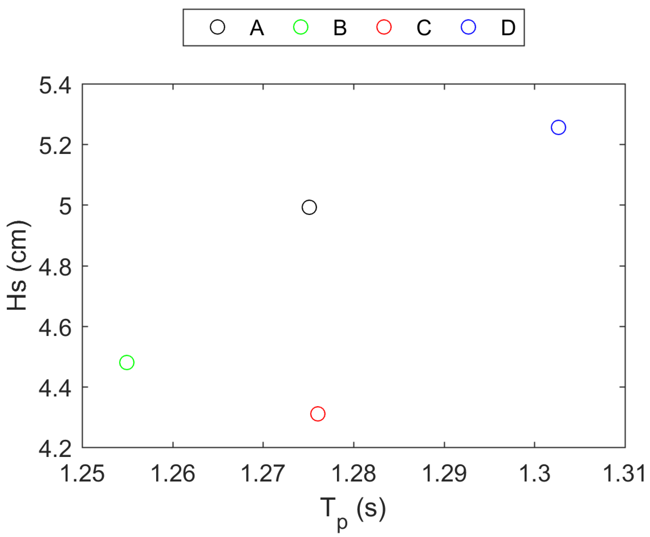
Figure 1. Theoretical JONSWAP spectrum T p = 1.29 s, H s = 5 cm and the eigen frequencies for surge, heave, and pitch.
Jmse 09 01030 g001
Figure 2. Motion responses to JONSWAP spectrum T p = 1.29 s, H s = 5 cm: in the low frequency range (left) and in the wave frequency range (right).
Jmse 09 01030 g002
Figure 3. Realised wave spectra for JONSWAP T p = 1.29 s and H s = 5 cm: in the low frequency range (left) and in the wave frequency range (right).
Jmse 09 01030 g003
Figure 4. Realised H s as function of realised T p for targeted JONSWAP T p = 1.29 s and H s = 5 cm sea-state.
Jmse 09 01030 g004
Figure 5. Ratio of realised ( H s r e a l ) to theoretical( H s t h e o ) significant wave height for targeted JONSWAP T p = 1.29 s, H s = 5 cm and 7.5 cm sea-state for facilities (AD).
Jmse 09 01030 g005
Figure 6. Ratio of realised ( S s r e a l ) to theoretical ( S s t h e o ) significant wave steepness for targeted JONSWAP T p = 1.29 , H s = 5 cm and 7.5 cm sea-sate for facilities (AD).
Jmse 09 01030 g006
Figure 7. Ratio of realised ( T p r e a l ) to theoretical ( T p t h e o ) peak wave period for targeted JONSWAP T p = 1.29 , H s = 5 cm and 7.5 cm sea-sate for facilities (AD).
Jmse 09 01030 g007
Figure 8. Metric T r (left column) and M W F (right column) for JONSWAP T p = 1.29 , H s = 5 cm for all facilities given for surge (top row), heave (middle row), and pitch (bottom row).
Jmse 09 01030 g008
Figure 9. Metric T r (left column) and M W F (right column) for JONSWAP T p = 1.29 , H s = 5 cm for all facilities given for the tensions in port mooring line ( T P S ; top row), starboard mooring line ( T S B ; middle row) and stern mooring line ( T S t ; bottom row).
Jmse 09 01030 g009
Figure 10. Metrics T r (left column) and M W F (right column) applied to surge (top row), heave (middle row), and pitch (bottom row) motions for JONSWAP T p = 1.81 s, H s = 15 cm in basins A, B, and C. The subscripts identify different seeds.
Jmse 09 01030 g010
Figure 11. Metrics T r (left column) and M W F (right column) applied to port side ( T P S , top row), starboard side ( T S B , middle row), and stern ( T S t , bottom row) mooring line tensions for JONSWAP T p = 1.81 s, H s = 15 cm in basins A, B, and C. The subscripts identify different seeds.
Jmse 09 01030 g011
Figure 12. Ratio of realised ( T p r e a l ) to theoretical ( T p t h e o ) peak period for targeted JONSWAP T p = 1.81 s, H s = 10 cm, and 15 cm sea-states for facilities (AD).
Jmse 09 01030 g012
Figure 13. Ratio of realised ( T p r e a l ) to theoretical ( T p t h e o ) peak period for targeted JONSWAP T p = 2.58 s, H s = 10 cm, 15 cm, and 20 cm sea-states for facilities (AD).
Jmse 09 01030 g013
Figure 14. Ratio of realised ( H s r e a l ) to theoretical ( H s t h e o ) significant wave height for targeted JONSWAP T p = 1.81 s, H s = 10 cm, and 15 cm sea-states for facilities (AD).
Jmse 09 01030 g014
Figure 15. Ratio of realised ( H s r e a l ) to theoretical ( H s t h e o ) significant wave height for targeted JONSWAP T p = 2.58 s, H s = 10 cm, 15 cm, and 20 cm sea-states for facilities (AD).
Jmse 09 01030 g015
Figure 16. Ratio of realised ( S s r e a l ) to theoretical ( S s t h e o ) wave steepness for targeted JONSWAP T p = 1.81 s, H s = 10 cm, and 15 cm sea-states for facilities (AD).
Jmse 09 01030 g016
Figure 17. Ratio of realised ( S s r e a l ) to theoretical ( S s t h e o ) wave steepness for targeted JONSWAP T p = 2.58 s, H s = 10 cm, 15 cm, and 20 cm sea-states for facilities (AD).
Jmse 09 01030 g017
Figure 18. Metrics T r (left column) and M W F (right column) applied to surge (top row), heave (middle row), and pitch (bottom row) motions for realised significant wave height ( H s r e a l ) with target JONSWAP T p = 1.29 s, H s = 5 cm, and 7.5cm sea-states per facility.
Jmse 09 01030 g018
Figure 19. Metrics T r (left column) and M W F (right column) applied to surge (top row), heave (middle row), and pitch (bottom row) motions for realised significant wave height ( H s r e a l ) with target JONSWAP T p = 1.81 s, H s = 10 cm, and 15 cm per facility.
Jmse 09 01030 g019
Figure 20. Metrics T r (left column) and M W F (right column) applied to surge (top row), heave (middle row), and pitch (bottom row) motions for realised significant wave height ( H s r e a l ) with target JONSWAP T p = 2.58 s, H s = 10 cm, 15 cm, and 20 cm sea-states per facility.
Jmse 09 01030 g020
Figure 21. Metrics T r (left column) and M W F (right column) for JONSWAP T p = 1.29 s, H s = 5 cm per facility for surge (top row), heave (middle row), and pitch (bottom row) at thrust levels of 0, 3, 5, 7, and 8 N (8 N applied at facility D only).
Jmse 09 01030 g021
Figure 22. Metrics T r (left column) and M W F (right column) for JONSWAP T p = 1.29 s, H s = 7.5 cm per facility for surge (top row), heave (middle row), and pitch (bottom row) at thrust levels of 0, 3, 5, 7, and 8 N (8 N applied at facility D only).
Jmse 09 01030 g022
Figure 23. Metrics T r (left column) and M W F (right column) for JONSWAP T p = 1.81 s, H s = 10 cm per facility for surge (top row), heave (middle row), and pitch (bottom row) at thrust levels of 0, 3, 5, 7, and 8 N (8 N applied at facility D only).
Jmse 09 01030 g023
Figure 24. Metrics T r (left column) and M W F (right column) for JONSWAP T p = 1.81 s, H s = 15 cm per facility for surge (top row), heave (middle row), and pitch (bottom row) at thrust levels of 0, 3, 5, 7, and 8 N (8 N applied at facility D only).
Jmse 09 01030 g024
Figure 25. Metrics T r (left column) and M W F (right column) for JONSWAP T p = 2.58 s, H s = 10, 15, and 20 cm for surge (top row), heave (middle row), and pitch (bottom row) at thrust levels of 0, 3, 5, 7, and 8 N for campaign D.
Jmse 09 01030 g025
Figure 26. Metrics T r (left column) and M W F (right column) for surge (top row), heave (middle row), and pitch (bottom row) for the Pink-Noise waves produced during campaigns D and E with thrust levels 0, 3, 5, 7, and 8 N.
Jmse 09 01030 g026
Table 1. List of test facilities.
FacilityReference
ECNA
IfremerB
UCC Campaign 1C
UoSD
UCC Campaign 2E
Table 2. Irregular wave list at model scale.
Spectrum Details T p (s) H s (m)Wind Thrust (N)Details
JONSWAP ( γ = 3.3 )1.290.050; 5; 7A, B, C, D
JONSWAP ( γ = 3.3 )1.290.053; 8D
JONSWAP ( γ = 3.3 )1.290.0750; 7A, B, C, D
JONSWAP ( γ = 3.3 )1.290.0753; 5; 8D
JONSWAP ( γ = 3.3 )1.810.100; 7A, B, C, D
JONSWAP ( γ = 3.3 )1.810.105A, B, D
JONSWAP ( γ = 3.3 )1.810.103C
JONSWAP ( γ = 3.3 )1.810.103; 8D
JONSWAP ( γ = 3.3 )1.810.150; 7A, B, C, D
JONSWAP ( γ = 3.3 )1.810.155A, B, D
JONSWAP ( γ = 3.3 )1.810.153C
JONSWAP ( γ = 3.3 )1.810.153; 8D
JONSWAP ( γ = 3.3 )2.580.100A, B, C, D
JONSWAP ( γ = 3.3 )2.580.103; 5; 7; 8D
JONSWAP ( γ = 3.3 )2.580.150A, B, C, D
JONSWAP ( γ = 3.3 )2.580.153; 5; 7; 8D
JONSWAP ( γ = 3.3 )2.580.200A, B, C, D
JONSWAP ( γ = 3.3 )2.580.203; 5; 7; 8D
Pink noise 0; 3; 5; 7; 8D, E
Table 3. Expected resonance responses for irregular wave conditions (low frequency (LF) or wave frequency (WF)) and WF range [ f 1 , f 2 ] (Hz) per wave condition.
Motion ModeSurgeHeavePitch f 1 f 2
JONSWAP T p = 1.29 sLFLFLF0.501.3
JONSWAP T p = 1.81 sLFWFLF0.351.2
JONSWAP T p = 2.58 sLFWFWF0.251.2
Pink-NoiseLFWFWF0.251.2
Table 4. Variations (%) of wave parameters and metrics across facilities for different random seed tests.
(Max-Min)/Mean (%)ABCA + B + C
Hs4.09.02.226.3
T p 1.02.11.43.6
Surge  T r 7.04.30.912.1
Heave  T r 1.01.71.42.8
Pitch  T r 1.20.61.91.9
Tension PS line  T r 7.64.11.312.2
Tension SB line  T r 6.44.43.811.4
Tension Stern line  T r 7.14.31.112.1
Surge  M W F 2.53.62.44.1
Heave  M W F 3.03.23.54.3
Pitch  M W F 4.35.62.86.1
Tension PS line  M W F 3.63.33.815.3
Tension SB line  M W F 4.53.71.717.8
Tension Stern line  M W F 3.13.72.34.1
Publisher’s Note: MDPI stays neutral with regard to jurisdictional claims in published maps and institutional affiliations.

