
A Unified Approach for Underwater Homing and Docking of over-Actuated AUV

Abstract
:1. Introduction
2. Problem Formulation
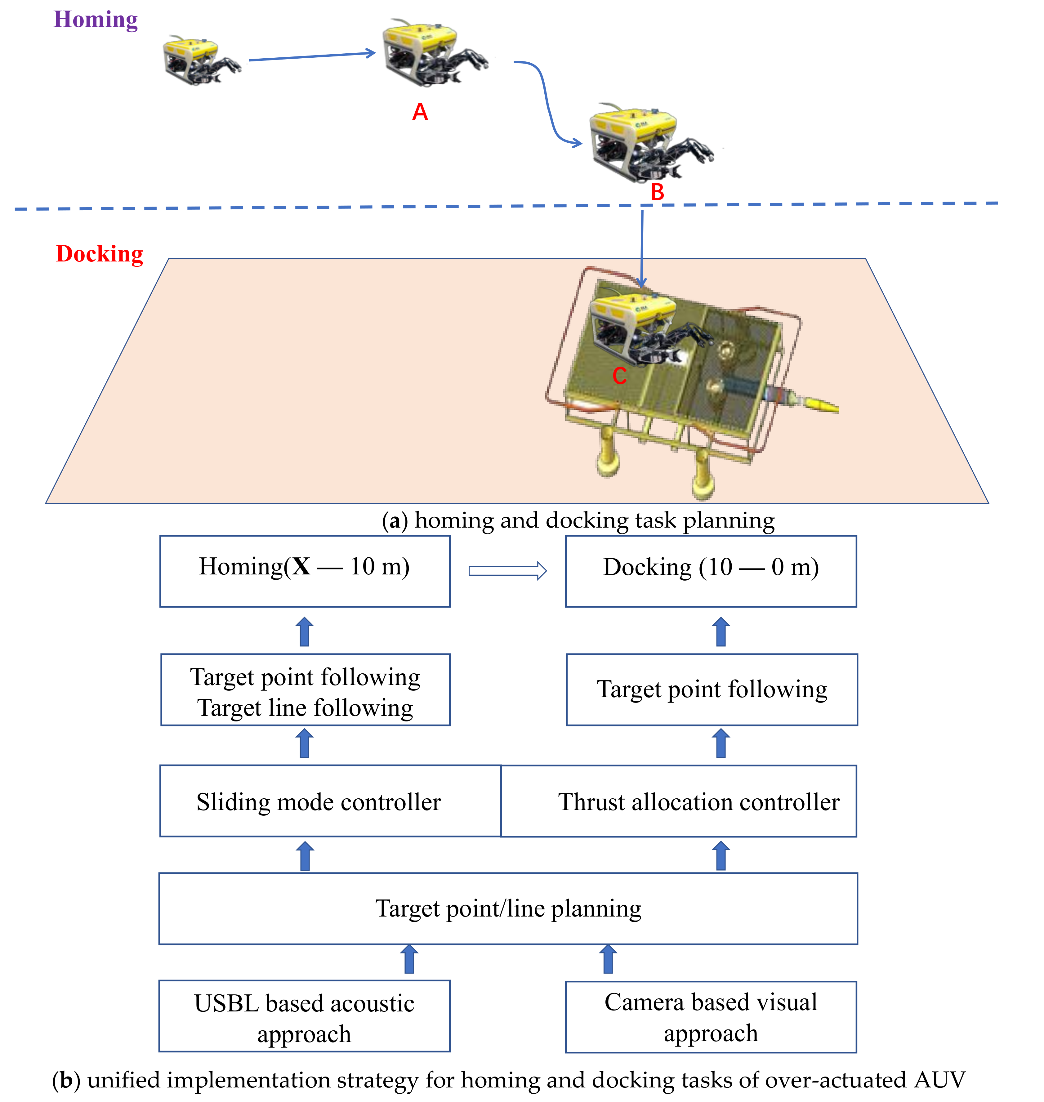
2.1. Description of Task Planning
2.2. Description of Guidance Design
2.3. Description of Controller Design
3. Homing and Docking Strategy
3.1. Task Planning
3.1.1. Homing Task
3.1.2. Docking Task
3.2. Guidance Design
3.2.1. Guidance for Homing
3.2.2. Guidance for Docking
- 1.
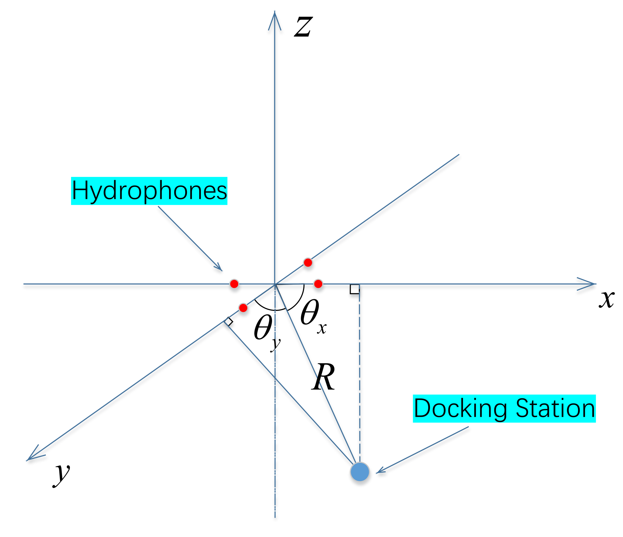
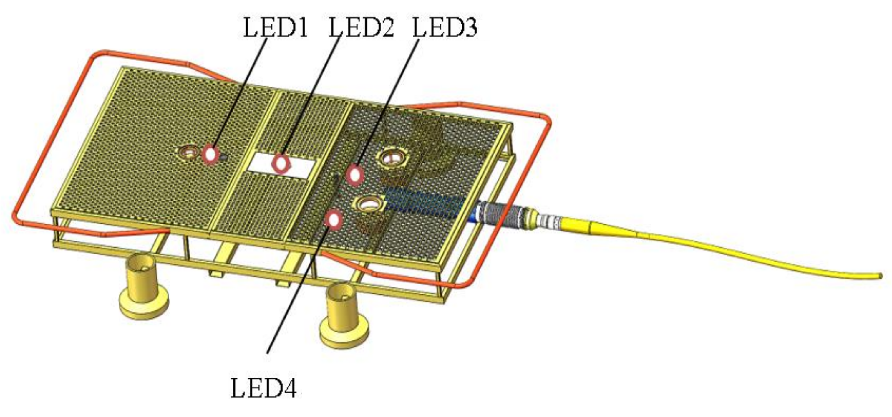
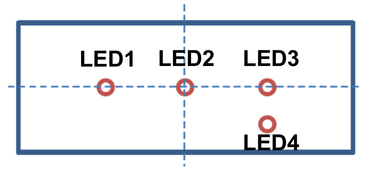
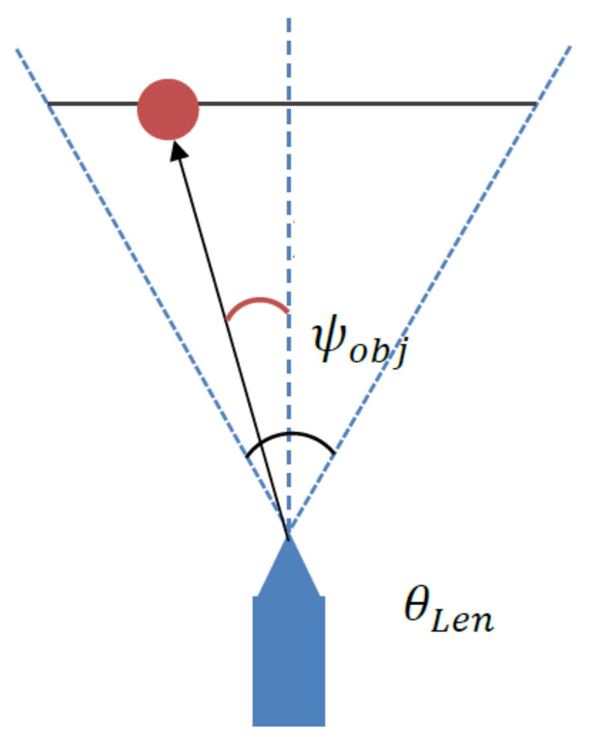
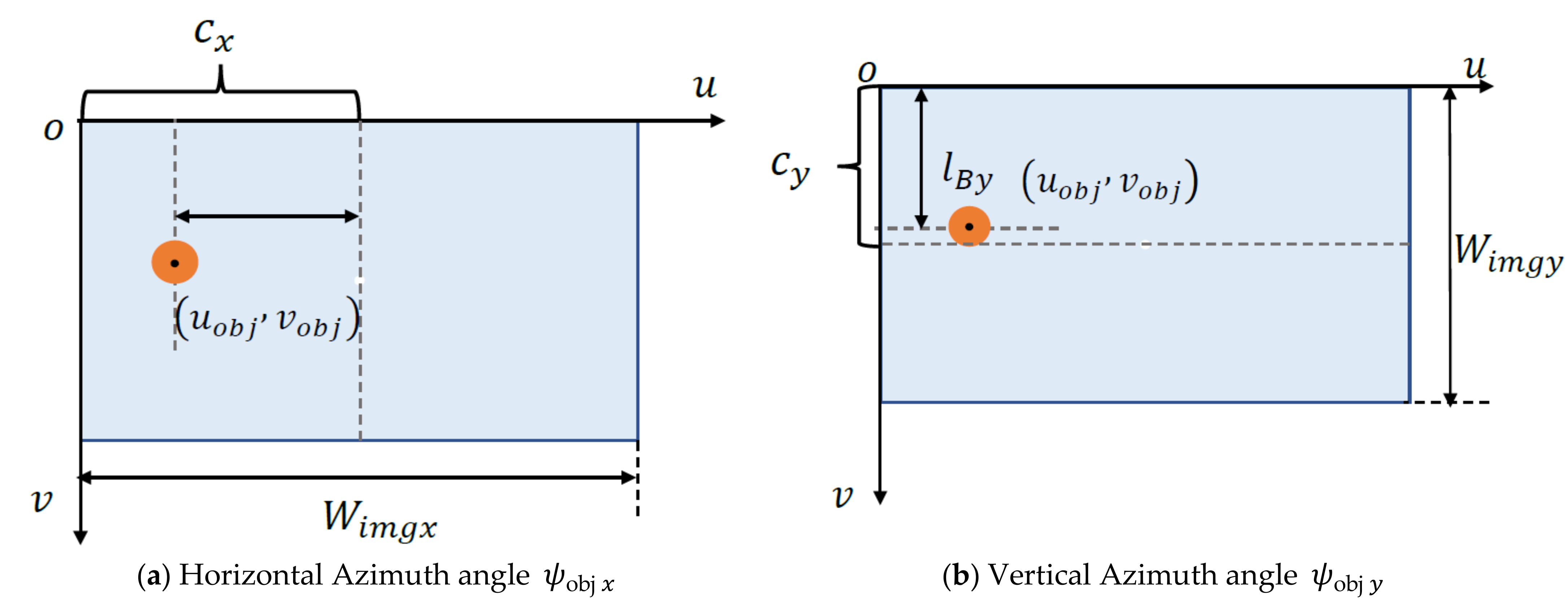
- Determine the relative position(x, ) between the DS center and the AUV bottom center (where the camera is). In determining the relative position(x, ) of the DS center, it is first necessary to determine the position of the DS center light, that is, LED2 in the light array in Figure 4. After the center position of each spot is calculated by the gray centroid method, four pixels are obtained, and the sum of the distances between each pixel and the other three pixels is calculated. The least sum of the distances is LED2, which is also the position of the DS center in the image. After determining the representative spot at the center of the DS, the azimuth angle can be calculated by using the geometric relationship (the azimuth of the target on the left side of the axis is negative, and the azimuth on the right side of the axis is positive) as shown in Figure 5. The angle between the projection of the line between the center of the DS and the camera on the horizontal plane with the camera axis and the camera axis is called the horizontal azimuth θLenx as shown in Figure 6a, then the horizontal azimuth of the DS center has the following relationship with the abscissa of the DS center in the image:
- 2.
- Determine the AUV yaw angle θ(Counterclockwise is positive, clockwise is negative). The deviation angle of the DS in the image needs to be determined. To calculate the location of the DS axis via the location of LED1, LED2, and LED3 in the light array, it is necessary to calculate the slope of the line between the pixel coordinates of three LED lights except for LED2 and LED2 in the image coordinate system, and then compare the three slopes. Then, the two lines with the closest slope will pass through LED1 and LED3 respectively, and the mean value of the slopes of the two lines will be treated as the slope of the DS axis in the image. The angle between the DS axis and the horizontal direction can be determined by the slope of the line. Then LED4 is used to determine the driving direction of AUV relative to the DS. The first is to determine the position of LED3 and calculate the distance between the three points on the line and the center of LED4. The closest point is the center of LED3. Here X2 and X3 are the pixel values of the abscissa of LED2 and LED3 in the center of the image respectively. If X2 > X3, the yaw angle of AUV θ = θ0, otherwise θ = 180° − θ0.
4. Controller Design
4.1. Dynamic Model
4.2. Sliding Mode Based Homing and Docking Control Design
4.2.1. Target Point Tracking
4.2.2. Target Line Tracking
5. Thrust Allocation
5.1. The Model of the Thrusters
5.2. Thrust Allocation Optimization
5.2.1. Problem Statement
5.2.2. QP Optimization
6. Simulation and Analysis
- ①
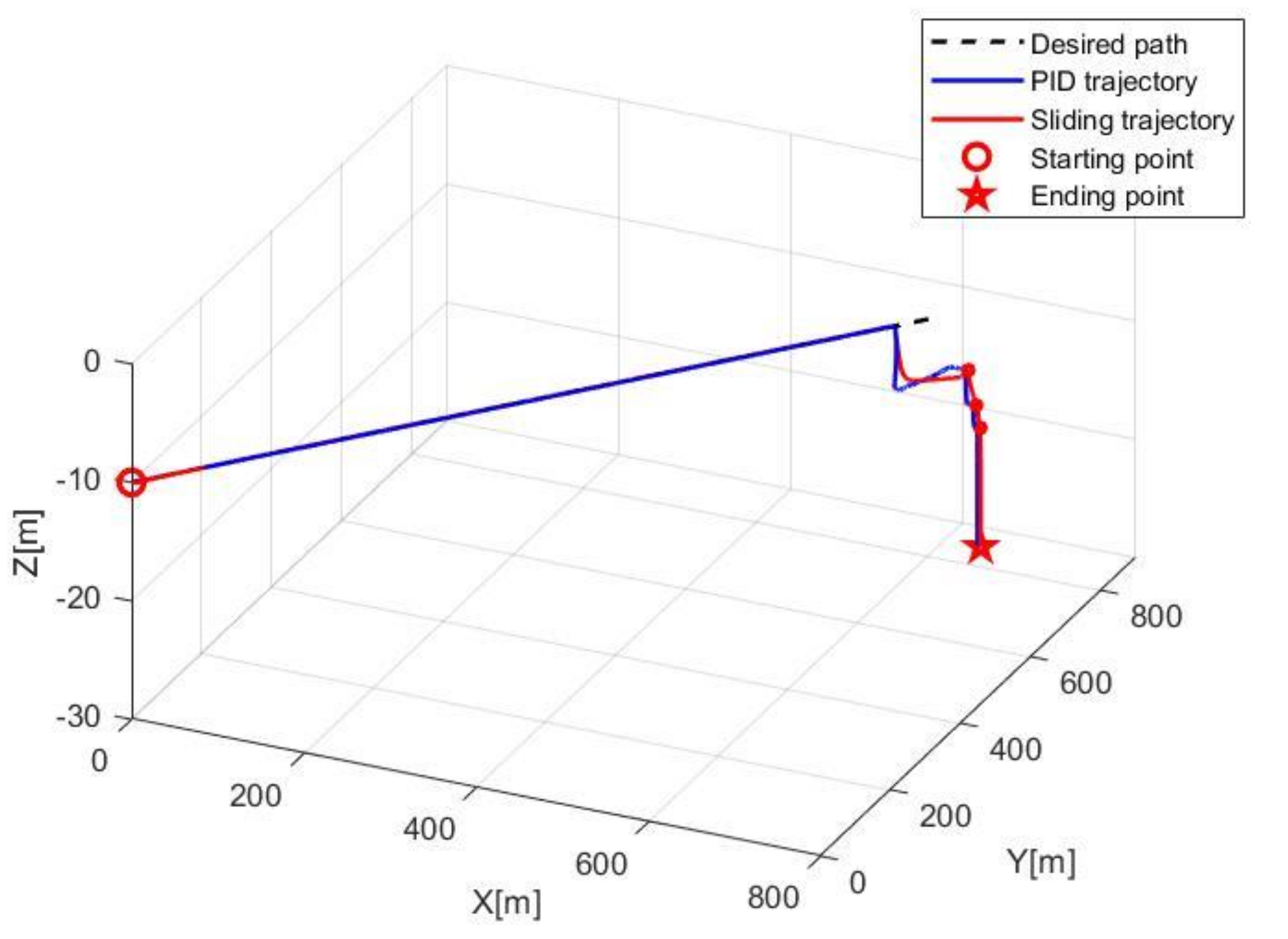
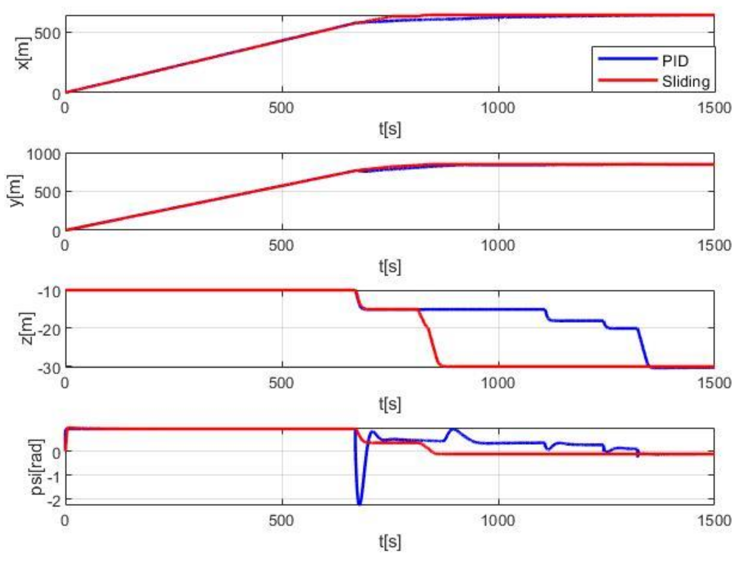
- P1 (600 m, 800 m, −10 m) is the target point information obtained by USBL at the initial time.
- ②
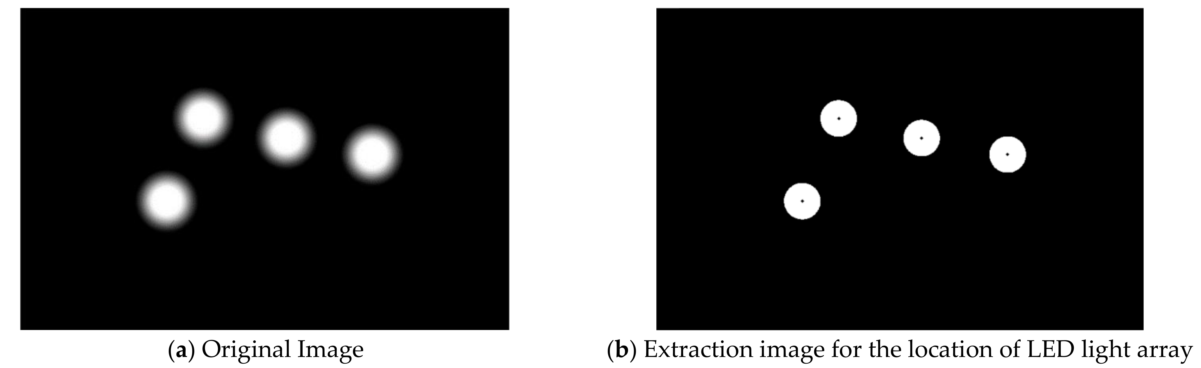
- P2 (630 m, 840 m, −15 m, 20°), P3 (637 m, 845 m, −18 m, 15°), P4 (640 m, 850 m, −20 m, 5°), The three target points are the planned target point information after the DS information is obtained by USBL after tracking to P1. P4 is the position 10 m above the DS. After the AUV tracks to P4, the image and processing information are obtained by the camera, as shown in Figure 9 and Table 2. The vision-based guidance is simulated on OpenCV. The accurate position P5 of the DS is obtained by the visual relative information.
- ③
- P5 (640.75 m, 848.68 m, −30 m, −7.03°), This point is the location information of the DS after the AUV arrives at P4 and performs fine target resolution by vision.
- ①
- Parameters for target line tracking
- ②
- Parameters for target point tracking
- ③
- Parameters for thruster allocation controller
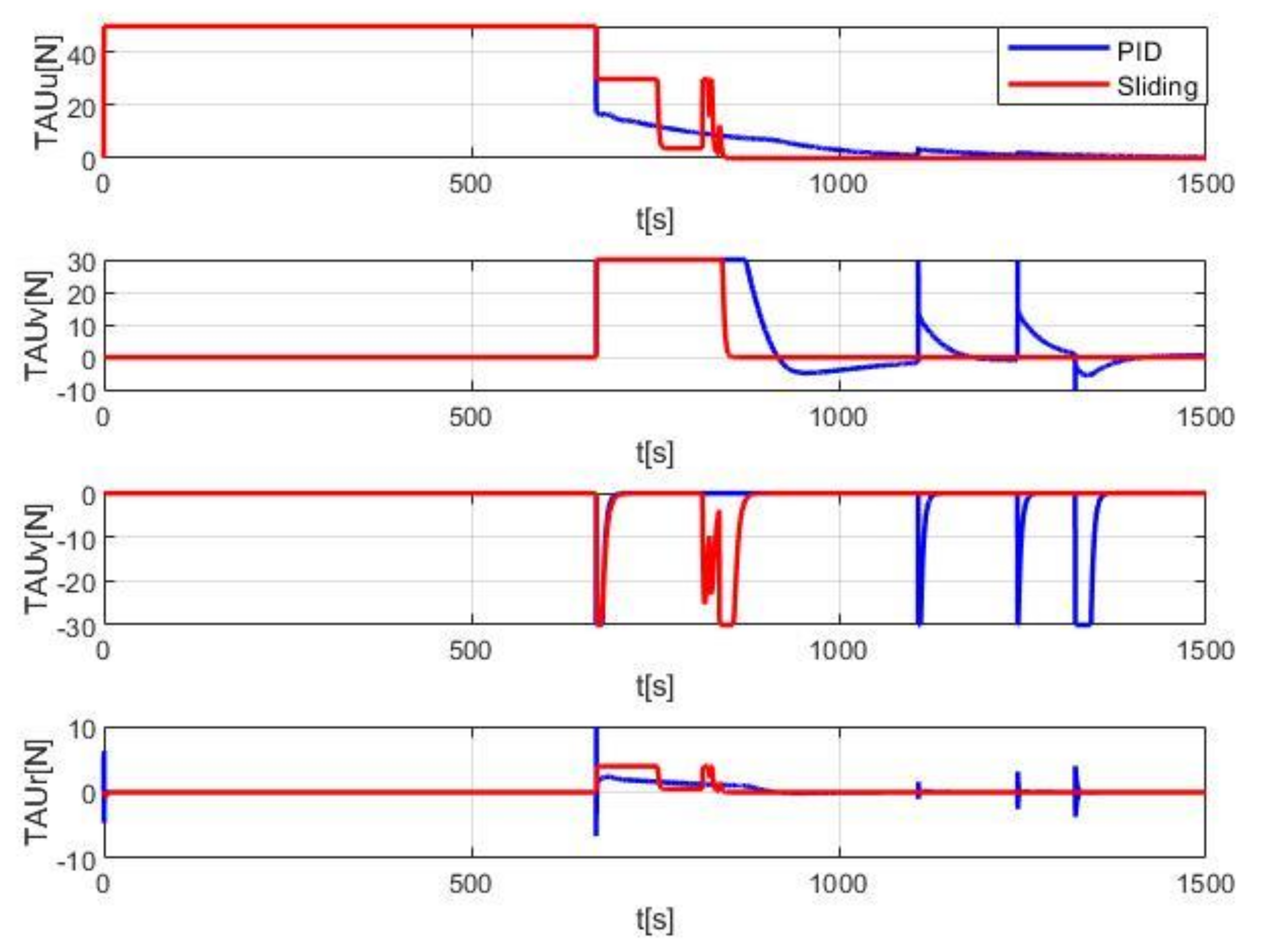
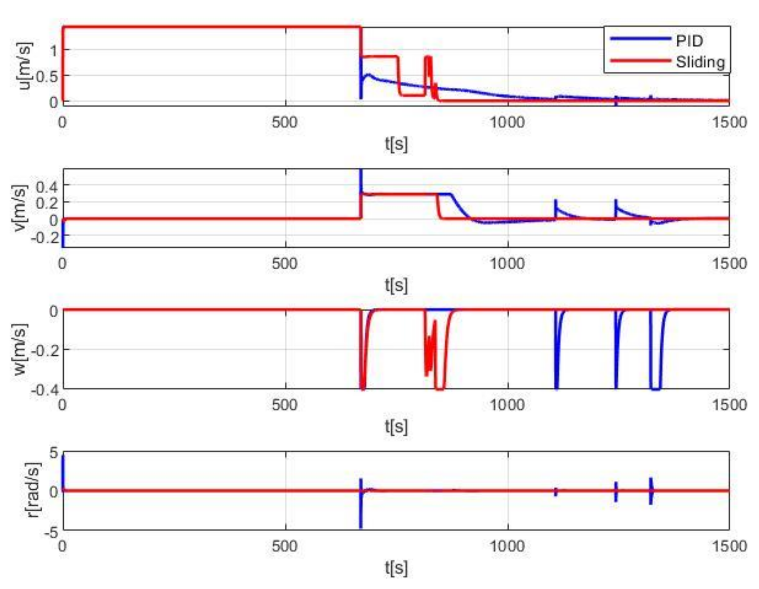
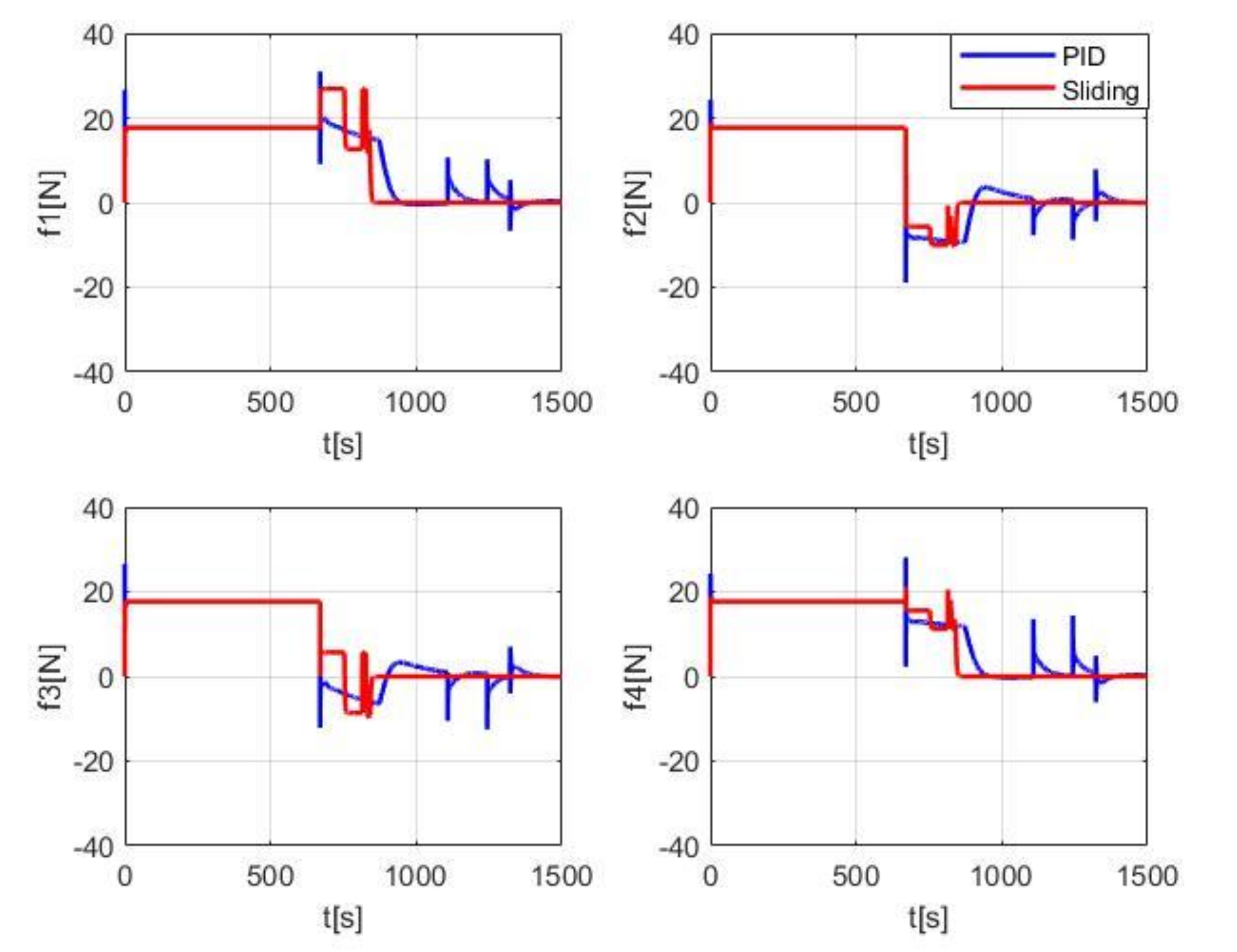
6.1. Simulation Results
6.2. Discussion and Analysis
7. Conclusions
Author Contributions
Funding
Institutional Review Board Statement
Informed Consent Statement
Data Availability Statement
Conflicts of Interest
References
- Newman, J.N. Marine Hydrodynamic; The MIT Press: Cambridge, MA, USA, 1977. [Google Scholar]
- Xiang, G.; Birk, L.; Yu, X.; Lu, H. Numerical Study on the Trajectory of Dropped Cylindrical Objects. Ocean Eng. 2017, 130, 1–9. [Google Scholar] [CrossRef]
- Wu, Y.; Li, L.L.; Su, X.C.; Gao, B.W. Dynamics modeling and trajectory optimization for unmanned aerial-aquatic vehicle diving into the water. Aerosp. Sci. Technol. 2019, 89, 220–229. [Google Scholar] [CrossRef]
- Xiang, G.; Xiang, X.B. 3D trajectory optimization of the slender body freely falling through water using Cuckoo Search Algorithm. Ocean Eng. 2021, 235, 109354. [Google Scholar] [CrossRef]
- Xiang, X.B.; Yu, C.Y.; Zhang, Q. On intelligent risk analysis and critical decision of underwater robotic vehicles. Ocean Eng. 2017, 140, 453–465. [Google Scholar] [CrossRef]
- Xiong, C.; Lu, D.; Zeng, Z.; Lian, L.; Yu, C. Path Planning of Multiple Unmanned Marine Vehicles for Adaptive Ocean Sampling Using Elite Group-Based Evolutionary Algorithms. J. Intell. Robot. Syst. 2020, 99, 875–889. [Google Scholar] [CrossRef]
- Peng, Z.H.; Gu, N.; Zhang, Y.; Liu, Y.J.; Wang, D.; Liu, L. Path-guided time-varying formation control with collision avoidance and connectivity preservation of under-actuated autonomous surface vehicles subject to unknown input gains. Ocean Eng. 2019, 191, 106501. [Google Scholar] [CrossRef]
- Xu, H.T.; Soares, C.G. Vector Field Guidance Law for Curved Path Following of an Underactuated Autonomous Ship Model. Int. J. Marit. Eng. 2020, 162, A249–A261. [Google Scholar]
- Qin, H.D.; Li, C.; Sun, Y.; Wang, N. Adaptive trajectory tracking algorithm of unmanned surface vessel based on anti-windup compensator with full-state constraints. Ocean. Eng. 2020, 200, 106906. [Google Scholar] [CrossRef]
- Xu, H.; Oliveira, P.; Soares, C.G. L1 adaptive backstepping control for path-following of underactuated marine surface ships. Eur. J. Control 2021, 58, 357–372. [Google Scholar] [CrossRef]
- Tao, J.; Sun, Q.L.; Tan, P.L.; Chen, Z.Q.; He, Y.P. Autonomous homing control of a powered parafoil with insufficient altitude. ISA Trans. 2016, 65, 516–524. [Google Scholar] [CrossRef]
- Martinsen, A.B.; Lekkas, A.M.; Gros, S. Autonomous docking using direct optimal control. IFAC-PapersOnLine 2019, 52, 97–102. [Google Scholar] [CrossRef]
- Li, J.J.; Xiang, X.B.; Yang, S.L. Robust adaptive neural network control for dynamic positioning of marine vessels with prescribed performance under model uncertainties and input saturation. Neurocomputing 2021, in press. [Google Scholar]
- Anderlini, E.; Parker, G.G.; Thomas, G. Docking Control of an Autonomous Underwater Vehicle Using Reinforcement Learning. Appl. Sci. 2019, 9, 3456. [Google Scholar] [CrossRef] [Green Version]
- Zhang, Q.; Zhang, J.L.; Chemori, A.; Xiang, X.B. Virtual Submerged Floating Operational System for Robotic Manipulation. Complexity 2018, 2018, 9528313. [Google Scholar] [CrossRef] [Green Version]
- Uchihori, H.; Cavanini, L.; Tasaki, M.; Majecki, P.; Yashiro, Y.; Grimble, M.J.; Yamamoto, I.; Molen, G.M.; Morinaga, A.; Eguchi, K. Linear Parameter-Varying Model Predictive Control of AUV for Docking Scenarios. Appl. Sci. 2021, 11, 4368. [Google Scholar] [CrossRef]
- Wang, Z.; Yu, C.; Li, M.; Yao, B.; Lian, L. Vertical Profile Diving and Floating Motion Control of the Underwater Glider Based on Fuzzy Adaptive LADRC Algorithm. J. Mar. Sci. Eng. 2021, 9, 698. [Google Scholar] [CrossRef]
- Bitar, G.; Martinsen, A.B.; Lekkas, A.M.; Breivik, M. Trajectory Planning and Control for Automatic Docking of ASVs with Full Scale Experiment. IFAC-PapersOnLine 2020, 53, 14488–14494. [Google Scholar] [CrossRef]
- Wang, Z.; Yang, S.; Xiang, X.; Vasilijević, A.; Mišković, N.; Nađ, Đ. Cloud-based mission control of USV fleet: Architecture, implementation and experiments. Control Eng. Pract. 2021, 106, 104657. [Google Scholar] [CrossRef]
- Peng, Z.H.; Wang, J.; Wang, D.; Han, Q.L. An overview of recent advances in coordinated control of multiple autonomous surface vehicles. IEEE Trans. Ind. Inform. 2021, 172, 732–745. [Google Scholar] [CrossRef]
- Peng, Z.H.; Liu, L.; Wang, J. Output-feedback flocking control of multiple autonomous surface vehicles based on data-driven adaptive extended state observers. IEEE Trans. Cybern. 2020, 1–12. [Google Scholar] [CrossRef]
- Roman, R.C.; Precup, R.E.; Bojan-Dragos, C.A.; Szedlak-Stinean, A.I. Combined model-free adaptive control with fuzzy component by virtual reference feedback tuning for tower crane systems. Procedia Comput. Sci. 2019, 162, 267–274. [Google Scholar]
- Turnip, A.; Panggabean, J.H. Hybrid controller design based magneto-rheological damper lookup table for quarter car suspension. Int. J. Artif. Intell. 2020, 18, 193–206. [Google Scholar]
- Precup, R.E.; Teban, T.A.; Oliveira, T.E.A.; Peria, E.M. Evolving fuzzy models for myoelectric-based control of a prosthetic hand. In Proceedings of the IEEE International Conference on Fuzzy Systems (FUZZ-IEEE), Vancouver, BC, Canada, 24–26 July 2016. [Google Scholar]
- Yazdani, A.M.; Sammut, K.; Yakimenko, O.; Lammas, A. A survey of underwater docking guidance systems. Robot. Auton. Syst. 2020, 124, 103382. [Google Scholar] [CrossRef]
- Anderson, N.A.; Bjerrum, A. Docking Capability of the MARTIN AUV. In Proceedings of the 5th IFAC Conference on Maneuvering and Control of Marine Craft, Aalborg, Denmark, 23–25 August 2000. [Google Scholar]
- Sans-Muntadas, A.; Brekke, E.F.; Hegrenæs, Ø.; Pettersen, K.Y. Navigation and Probability Assessment for Successful AUV Docking Using USBL. IFAC-PapersOnLine 2015, 48, 204–209. [Google Scholar] [CrossRef]
- Vandavasi, B.N.; Arunachalam, U.; Narayanaswamy, V.; Raju, R.; Vittal, D.R.; Muthiah, R.K.; Gidugu, A.R. Concept and testing of an electromagnetic homing guidance system for autonomous underwater vehicles. Appl. Ocean Res. 2018, 73, 149–159. [Google Scholar] [CrossRef]
- Yahya, M.F.; Arshad, M.R. Tracking of Multiple Light Sources Using Computer Vision for Underwater Docking. Procedia Comput. Sci. 2015, 76, 192–197. [Google Scholar] [CrossRef] [Green Version]
- Trslic, P.; Rossi, M.; Robinson, L.; O’Donnel, C.W.; Weir, A.; Coleman, J.; Riordan, J.; Omerdic, E.; Dooly, G.; Toal, D. Vision based autonomous docking for work class ROVs. Ocean Eng. 2020, 196, 106840. [Google Scholar] [CrossRef]
- Li, Y.; Jiang, Y.Q.; Cao, J.C.; Wang, B.; Li, Y.M. AUV docking experiments based on vision positioning using two cameras. Ocean Eng. 2015, 110, 163–173. [Google Scholar] [CrossRef]
- Vallicrosa, G.; Bosch, J.; Palomeras, N.; Ridao, P.; Carreras, M.; Gracias, N. Autonomous homing and docking for AUVs using Range-Only Localization and Light Beacons. IFAC-PapersOnLine 2016, 49, 54–60. [Google Scholar] [CrossRef]
- Yang, C.J.; Peng, S.L.; Fan, S.S.; Zhang, S.Z.; Wang, P.F.; Chen, Y. Study on docking guidance algorithm for hybrid underwater glider in currents. Ocean Eng. 2016, 125, 170–181. [Google Scholar] [CrossRef]
- Breivik, M.; Loberg, J.E. A Virtual Target-Based Underway Docking Procedure for Unmanned Surface Vehicle. In Proceedings of the 18th World Congress. The International Federation of Automatic Control, Milano, Italy, 28 August–2 September 2011. [Google Scholar]
- Wang, N.; Wang, Y.; Er, M. Review on deep learning techniques for marine object recognition: Architectures and algorithms. Control Eng. Pract. 2020, 104458. [Google Scholar] [CrossRef]
- Park, J.Y.; Jun, B.H.; Lee, P.M.; Oh, J.O. Experiments on vision guided docking of an autonomous underwater vehicle using one camera. Ocean Eng. 2009, 36, 48–61. [Google Scholar] [CrossRef]
- Li, D.J.; Chen, Y.H.; Shi, J.G.; Yang, C.J. Autonomous underwater vehicle docking system for cabled ocean observatory network. Ocean Eng. 2015, 109, 127–134. [Google Scholar] [CrossRef]
- Palomeras, N.; Vallicrosa, G.; Mallios, A.; Bosch, J.; Vidal, E.; Hurtos, N.; Carreras, M.; Ridao, P. AUV homing and docking for remote operations. Ocean Eng. 2018, 154, 106–120. [Google Scholar] [CrossRef]
- Matsuda, T.; Maki, T.; Masuda, K.; Sakamaki, T. Resident autonomous underwater vehicle: Underwater system for prolonged and continuous monitoring based at a seafloor station. Robot. Auton. Syst. 2019, 120, 103231. [Google Scholar] [CrossRef]
- Wang, T.L.; Zhao, Q.C.; Yang, C.J. Visual navigation docking and charging system. Ocean Eng. 2021, 224, 108744. [Google Scholar] [CrossRef]
- Ferreira, B.; Matos, A.C.; Cruz, N.A.; Moreira, A.P. Homing a robot with range-only measurements under unknown drifts. Robot. Auton. Syst. 2015, 67, 3–13. [Google Scholar] [CrossRef]
- Thomas, C.; Simetti, E.; Casalino, G. A Unifying Task Priority Approach for Autonomous Underwater Vehicles Integrating Homing and Docking Maneuvers. J. Mar. Sci. Eng. 2021, 9, 162. [Google Scholar] [CrossRef]
- Brian, R.P.; Reeve, L.; Jalil, C.-G.; Nina, M. Underwater Docking Approach and Homing to Enable Persistent Operation. Front. Robot. AI 2021, 8, 621755. [Google Scholar] [CrossRef]
- Liao, K.P.; Hu, C.H.; Sueyoshi, M. Free surface flow impacting on an elastic structure: Experiment versus numerical simulation. Appl. Ocean Res. 2015, 50, 192–208. [Google Scholar] [CrossRef]
- Xiang, G.; Guedes Soares, C. Improved dynamical modelling of freely falling underwater cylinder based on CFD. Ocean Eng. 2020, 211, 107538. [Google Scholar] [CrossRef]
- Zhang, X.Y.; Shi, Y.; Pan, G. Stress control of cylinders during water entry based on the characteristics of bi-material interfaces. Ocean Eng. 2020, 214, 107723. [Google Scholar] [CrossRef]
- Xiang, G.; Wang, S.; Guedes Soares, C. Study on the Motion of a Freely Falling Horizontal Cylinders into Water Using OpenFOAM. Ocean Eng. 2020, 196, 106811. [Google Scholar] [CrossRef]


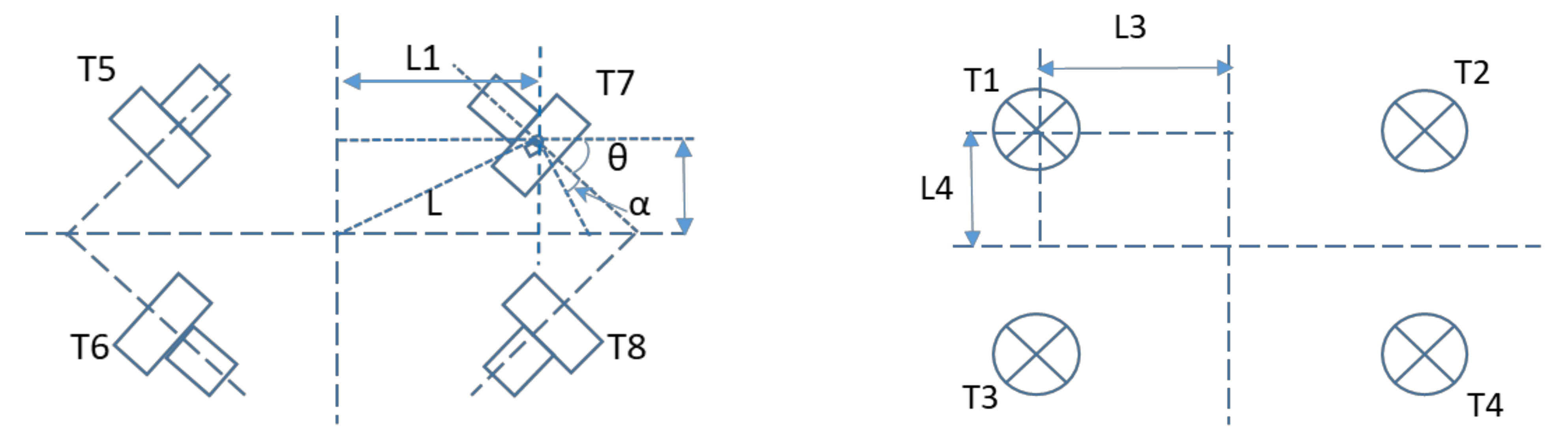
| NO. | Location | Azimuth | |||
|---|---|---|---|---|---|
| X | Y | Z | |||
| 1 | L3 | L4 | Z2 | 0 | 90 |
| 2 | L3 | L4 | Z2 | 0 | −90 |
| 3 | L3 | L4 | Z2 | 0 | −90 |
| 4 | L3 | L4 | Z2 | 0 | 90 |
| 5 | 45 | 0 | |||
| 6 | −45 | 0 | |||
| 7 | −45 | 0 | |||
| 8 | 45 | 0 | |||
| - | (m) | (m) | ||||
|---|---|---|---|---|---|---|
| Calculated value | 4.3056 | −7.5379 | 0.7529 | −1.3233 | −12.0340 | −12.0340 |
| True value | 4.3056 | −7.3758 | 0.7529 | −1.2945 | −12.6515 | −12.6515 |
| Relative error | 0 | 2.20% | 0 | 2.15% | −4.88% | −4.88% |
Publisher’s Note: MDPI stays neutral with regard to jurisdictional claims in published maps and institutional affiliations. |
© 2021 by the authors. Licensee MDPI, Basel, Switzerland. This article is an open access article distributed under the terms and conditions of the Creative Commons Attribution (CC BY) license (https://creativecommons.org/licenses/by/4.0/).
Share and Cite
Zuo, M.; Wang, G.; Xiao, Y.; Xiang, G. A Unified Approach for Underwater Homing and Docking of over-Actuated AUV. J. Mar. Sci. Eng. 2021, 9, 884. https://doi.org/10.3390/jmse9080884
Zuo M, Wang G, Xiao Y, Xiang G. A Unified Approach for Underwater Homing and Docking of over-Actuated AUV. Journal of Marine Science and Engineering. 2021; 9(8):884. https://doi.org/10.3390/jmse9080884
Chicago/Turabian StyleZuo, Mingjiu, Guandao Wang, Yongxin Xiao, and Gong Xiang. 2021. "A Unified Approach for Underwater Homing and Docking of over-Actuated AUV" Journal of Marine Science and Engineering 9, no. 8: 884. https://doi.org/10.3390/jmse9080884
APA StyleZuo, M., Wang, G., Xiao, Y., & Xiang, G. (2021). A Unified Approach for Underwater Homing and Docking of over-Actuated AUV. Journal of Marine Science and Engineering, 9(8), 884. https://doi.org/10.3390/jmse9080884