Article

Research on the Blade Motion of a Bidirectional Energy-Generating Turbine under Integrated Wave and Tidal Current Action

1
School of Mechanical Engineering, Tongji University, Shanghai 201804, China
2
Shanghai Marine Highend Equipment Functional Platform Co., Ltd., Shanghai 201306, China
3
School of Engineering, Shanghai Ocean University, Shanghai 201306, China
*
Authors to whom correspondence should be addressed.
J. Mar. Sci. Eng. 2021, 9(8), 869; https://doi.org/10.3390/jmse9080869
Submission received: 3 July 2021 / Revised: 7 August 2021 / Accepted: 10 August 2021 / Published: 12 August 2021
(This article belongs to the Section Ocean Engineering)

Abstract

:
An integrated wave-tidal current power turbine is affected by both wave and tidal current forces, and its energy efficiency is closely related to the velocity and direction of the two forces. To improve the probability of the horizontal axis turbine reaching maximum energy efficiency under real-time changing sea conditions, we performed the following investigations in this study. Based on the actual application scenario of Lianyungang port, a time series prediction model of tidal current (velocity and flow direction) and wave (mean wave direction, mean wave period, and significant wave height) data for the past year was established. The changes in waves and tidal currents within 24 h after the cutoff point of the existing data were predicted. The integrated wave-tidal current mechanism was studied, and the superposition of wave energy and tidal current energy was transformed into the equivalent velocity vector of wave-tidal current integration. The conversion coefficient between waves and equivalent flows was determined by a numerical wave flume simulation. According to the historical wave and tidal current data, the equivalent velocity range of the integrated action of waves and tidal currents in Lianyungang was determined. The influence of different blade motions on the energy harvesting efficiency of the turbine under the corresponding flow conditions was studied using the Computational Fluid Dynamics (CFD) method to determine the blade motion law of the turbine. The blade motion law of the prototype was verified in a sea trial experiment. The experimental results were basically consistent with the simulation results for the blade motion law designed according to the wave and tidal current prediction law. This design scheme can provide a reference for engineering design for the development and utilization of new marine energy.

1. Introduction

In the development and utilization of renewable marine energy, tidal current energy [1,2] and wave energy [3] are not only a research focus with high technological maturity but are also a hotspot of engineering applications. The two are inseparable and have an integrated effect. For example, suspended tidal turbines can obtain tidal current energy at large velocities near the sea, but are also affected by surface waves. Ethan et al. [4] studied the influence of surface gravity waves on the performance of tidal current turbines. The results showed that waves yield a small increase in turbine performance which can be explained by Stokes drift velocity. Lu et al. [5] analyzed the performance influence of vertical axis tidal current turbines under waves and tidal currents through experiments, and proved that the presence of waves increased the output power of tidal current turbines and improved their power generation performance. The tidal energy turbine designed by Wang et al. [6] from Shanghai Ocean University increased the absorbed power by 23 W under the combined action of waves and tidal currents compared with that under the same flow conditions, and the energy acquisition efficiency was increased by one percentage point. Therefore, the integration and collaboration of wave energy and tidal current energy into the same operating system can strengthen the multi-energy interconnection, promote the complementary advantages of multiple energy sources, improve the power generation per unit volume of sea area, and output a more stable performance. It can reduce the use of standby power generation equipment in renewable energy power generation, which not only reduces costs but is also beneficial for environmental protection.
Domestic and foreign scholars have conducted a great deal of research on the combined action mechanism of tidal current energy and wave energy. In 1987, Hedges [7] formally proposed the concept and preliminary structure of wave and tidal current integrated power generation, and integrated power generation technology began to develop. With the development of research technology, various types of wave and tidal current energy integration devices are emerging. Omar et al. [8] carried out research on wave-tidal current interaction theory and power generation technology, as well as many prototype experiments. Draycott et al. [9] carried out a nonlinear wave load test of a horizontal axis tidal current turbine and studied the influence of waves on tidal current turbines by using a 1:15 scale pool model. However, the development of wave and tidal current integration technology in China has lagged behind that of other countries [10,11]. In 2011, Shanghai Ocean University first proposed an integrated wave-tidal current power generation scheme and developed an integrated marine wave-tidal current power generation device with a single-unit capacity of no less than 500 W [12]. However, a complete theoretical system of resource evaluation and the mechanism of wave-tidal current integration have not been established. There are still problems such as the low energy conversion efficiency and poor reliability of wave-tidal current integrated power generation devices, and there are still numerous hurdles to clear before the large-scale promotion and application of such devices [13,14]. Therefore, the research on the mechanism of wave-current integration is of great significance for the improvement of the energy harvesting efficiency of the wave-tidal current integrated power generation turbine.
Many studies show that horizontal axis blades of tidal current turbines have a higher power generation efficiency and self-starting performance than turbines with vertical axis blades [15,16,17,18]. In the design of a horizontal axis tidal current energy turbine, a variable-pitch turbine can adapt to changes in tidal current velocity and direction by adjusting the blade declination to improve the self-starting performance and energy acquisition efficiency of the turbine [19,20]. However, most variable-pitch turbines do not consider the role of wave integration in the design process of blade motion law, and actual sea conditions are more complex than a single tidal current. Therefore, improving the energy efficiency of variable-pitch turbines under the action of wave-tidal current integration remains a challenge, and the posture change law of the turbine should be designed according to the characteristics of wave-tidal current integration. International scholars have conducted limited research on the variable posture law of horizontal axis turbines under wave-tidal current combined action. At the same time, for a determined sea area, tidal currents and waves have certain rules. The tidal current has strong periodicity, and waves also show certain cyclical fluctuation with the seasons [21]. The data have a strong correlation in the time scale, but the time series of waves and tidal currents are nonlinear, and a simple linear regression method cannot be used for prediction. It is necessary to select a more effective prediction model according to the characteristics of waves and tidal currents parameters to predict the variation of waves and tidal currents and provide a reference for the design of blade motion law.
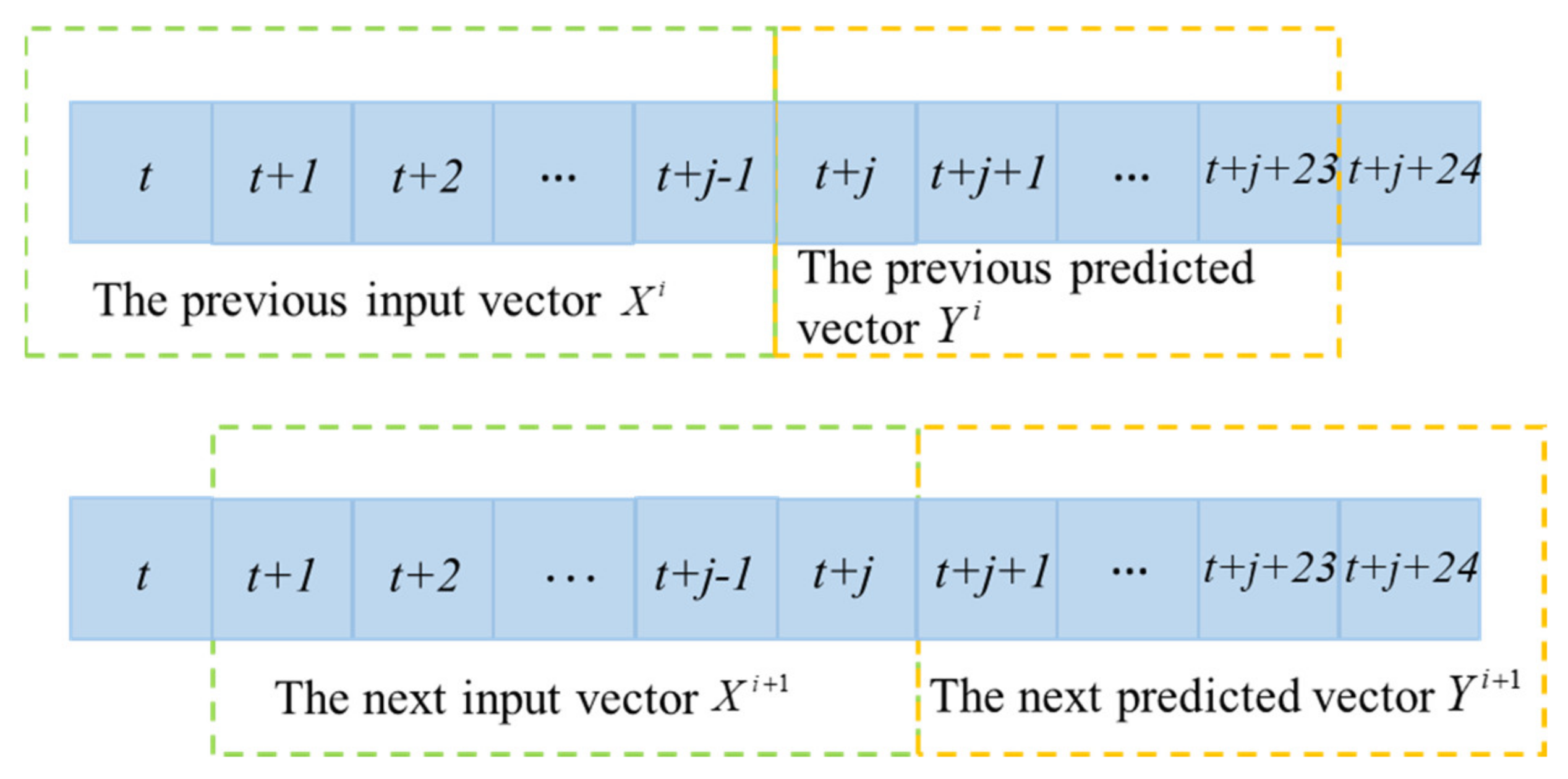
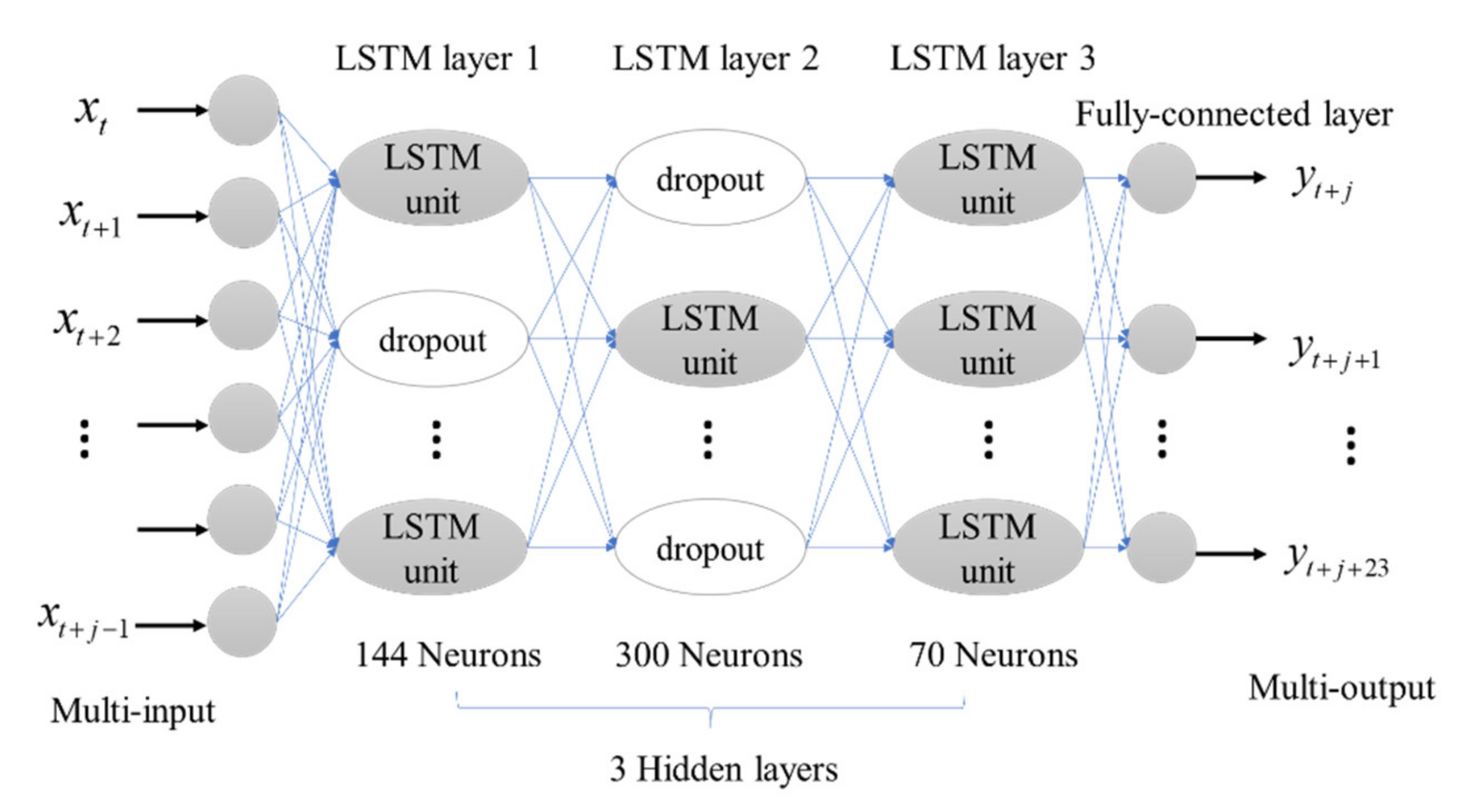
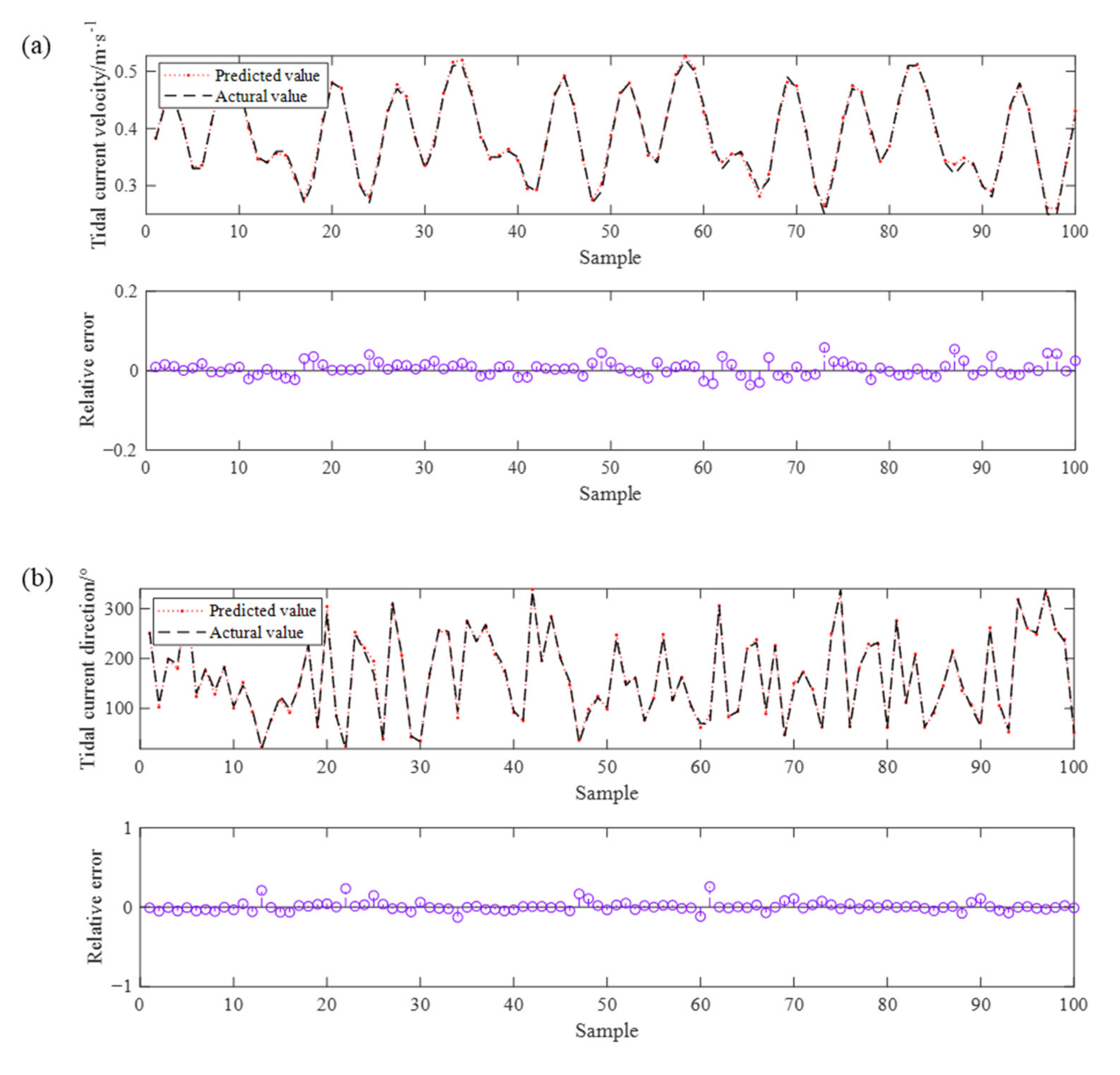
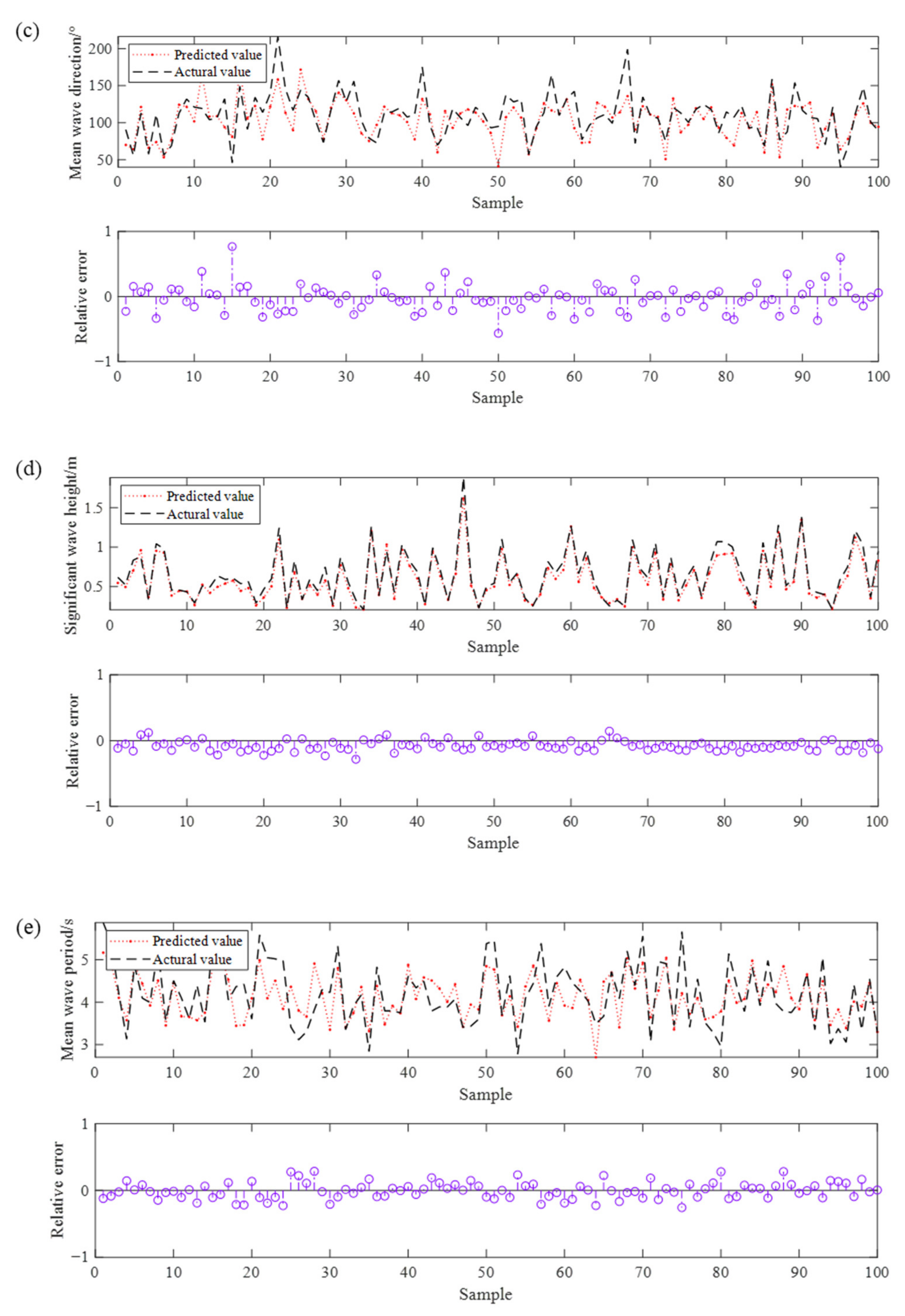
In this paper, we propose a design method of blade motion law based on the prediction of the change law of waves and tidal currents, so that the horizontal axis turbine can achieve the maximum energy harvesting efficiency at different times and under different working conditions. We take the S-foil bidirectional energy harvesting horizontal axis turbine as the study object and Lianyungang port as the practical application scenario. Through an analysis of the open tidal current and wave data from the past year, the neural network prediction model of wave (mean wave direction, mean wave period, and significant wave height) and tidal current (velocity and direction) data is constructed to predict the change law of waves and tidal currents within 24 h after the existing data cutoff point. On this basis, a mathematical model of the mechanism of wave-tidal current integration is deduced and established. Since the turbine mainly captures the kinetic energy generated by the lateral inflow, the complex mechanism of wave-tidal current integration is simplified in this paper, and the wave-tidal current integration is converted into an equivalent tidal current velocity vector so that forces on the turbine in all directions are integrated into the lateral force to better study the hydrodynamic performance of the horizontal axis turbine. This equivalent vector is related to tidal current velocity, tidal current direction, mean wave direction, mean wave period, and significant wave height. Then, the conversion coefficient of waves and equivalent flows is determined by numerical wave tank experiments, and the equivalent velocity range of wave-tidal current integration in Lianyungang port is determined. Finally, the influence of different blade deflection angles on the energy harvesting efficiency of the turbine under different flow conditions is studied by the CFD method to determine the variable attitude law of the turbine, which is verified in a sea trial experiment. Compared with the S-foil horizontal axis turbine previously designed by our research group [22], the variable-pitch turbine proposed in this paper adopts the blade motion law designed based on the prediction of the change law of waves and tidal currents, which not only ensures the acquisition of tidal current energy, but also integrates the wave energy, so that the energy acquisition efficiency under the same flow condition is increased by about 10%. In addition, this study provides a new method for the engineering design of new marine energy development and utilization, and provides a new idea for the improvement of power generation efficiency.
This paper is organized as follows. The prediction of the change law of waves and tidal currents according to the existing data of Lianyungang is presented in Section 2. The mathematical mechanism of wave-tidal current integration according to the physical characteristics of wave and tidal current is presented in Section 3. The blade motion law of the turbine is studied in Section 4, together with the details of CFD simulations. Section 5 shows the sea trial results of the prototype turbine. Finally, the conclusions of this paper are presented in Section 6.

2. Prediction of Waves and Tidal Currents

Tidal current velocity, tidal current direction, mean wave direction, mean wave period, and significant wave height are five parameters with high correlations with dynamic seawater acquisition that have a certain periodicity and are independent of each other. As a powerful recurrent neural network, Long-term and Short-term Memory (LSTM) can maintain an internal input memory, compensating for the gradient disappearance and gradient explosion problems present in the training process of Recurrent Neural Network (RNN). LSTM can effectively solve the problem of correlation between data before and after processing and can be widely used for the prediction of periodic time series data [23,24]. Therefore, an LSTM model based on the five columns of data is established to predict tidal current and wave data within 24 h after the cutoff point of the existing data.

2.1. Characteristics of the LSTM Neural Network

In this study, an LSTM neural network, which is a kind of artificial neural network (ANN) that includes the time cycle structure in deep learning and can accurately model time series data, was used. In the calculation of the LSTM neural network model, past iterations and samples are remembered, which can affect the current decision. The current and past input data as well as the past LSTM neural network computation state are considered as the input to solve the current output. Therefore, the time series needs to be discretized with equal time steps, dt, and the output of the training model is as follows:
y o = g ( V , s t ) = V · f ( U · x t + c t 1 + W · s t 1 ) = V · f ( U · x t + c t 1 + W · f ( U · x t 1 + c t 2 + W · s t 2 ) ) = V · f ( U · x t + c t 1 + W · f ( U · x t 1 + c t 2 + W · f ( U · x t 2 + ) ) )
where g(*) is the activation function of the output layer, V is the weight matrix of the output layer, and st is the calculation formula of the hidden layer, which includes three types of input, namely, the current input layer xt, the input of the hidden layer at the previous time step st−1, and the status of the neuron at the previous time step ct−1. f(*) is the activation function of the hidden layer, U is the synaptic weight matrix from the input layer to the hidden layer, and W is the synaptic weight matrix from st−1 to the hidden layer at this time step.

2.2. Construction of Prediction Model

The tidal current (velocity, direction) and wave (mean wave direction, mean wave period, and significant wave height) data of Lianyungang station from June 2020 to June 2021 were obtained from the National Ocean Information Center and the European Centre for Medium-Range Weather Forecasts Re-Analysis-5 (ERA5) reanalysis database, respectively. The ratio of the training set to the test set for each single column of data was set to 8:2. The input and output of the training model were constructed by using the recursive structure of the sliding window. Compared with the training samples of traditional structures, the training samples of the recursive structure were trained by multiple time data, ensuring the time coupling of the input and output. Let X i be the vector that constitutes the input and Y i be the vector that constitutes the output. The number of vectors is i, the length of the input window is j(j < t), the window length is the number of input steps, and the number of output steps is 24. The prediction diagram of the recursive structure is shown in Figure 1.
A stacked LSTM network composed of three hidden layers was constructed to train single-column data, and the dropout algorithm was used to improve the generalization ability and robustness of the model. The changes in tidal currents and waves within 24 h after the existing data cutoff point could thus be predicted. The model structure of the LSTM network is shown in Figure 2. In the multistep prediction process, LSTM was expanded into a feed-forward neural network, and the input vector and output vector were acquired from the first moment in a circular way, thus forming the input vector set X i n and the output vector set Y o u t .
The model accuracy (acc), coefficient of determination (R2), and root mean square error (RMSE) are used to evaluate the model. The calculation equations [25] are as follows.
The acc is as follows:
a c c = 1 i = 1 n e i i = 1 n y i × 100 %
where e i = y ^ i y i is the calculation error, y ^ i is the predicted value, and y i is the actual value.
The RMSE is as follows:
R M S E = 1 n i = 1 n y ^ i y i 2
The R2 is as follows:
R 2 = i = 1 n ( y ^ i y ¯ ) 2 i = 1 n ( y i y ¯ ) 2
where y ¯ is the average value.
To accelerate the convergence speed of neural network training and improve the computational efficiency, the data need to be normalized, and the expression is as follows:
x = x x min x max x min
where x max and x min are the maximum and minimum values of the sample data.

2.3. Analysis of Prediction Results

As shown in Figure 3, the trained model is applied to the test set, and 100 samples are randomly selected to compare the predicted value with the real value. The prediction accuracies of the five time series datasets are 0.98, 0.94, 0.92, 0.90, and 0.97. The R2 values are 0.92, 0.91, 0.90, 0.96, and 0.93. The RMSE values are 0.01, 7.73, 14.96, 0.08, and 0.38. The prediction accuracies of the five time series datasets are greater than 90%, and the highest accuracy is 98%, meaning that the prediction results are good. The RMSE values of the tidal current direction and mean wave direction are both larger than that of the other three datasets. This is because the direction range of waves and tidal currents is 0°–360°, and its absolute error is relatively large relative to that of the mean wave period, significant wave height, and tidal current velocity. Therefore, the RMSE values cannot fully characterize the quality of the prediction model. In combination with the relative errors and R2 values in Figure 3b,c, it can be seen that the trends of the predicted value and the real value curves are similar, the relative errors of tidal current direction and mean wave direction are small. In addition, the R2 values of five datasets are greater than 90%, indicating that the input and output of the LSTM model are strongly correlated, and the independent variables selected in the prediction model can explain more than 90% of the dependent variables. In summary, this prediction model can accurately predict the changes in tidal currents and waves within 24 h after the existing data cutoff point. In the practical application process, the wave and tidal current data of the past 72 h can be collected from official websites to continuously predict their changes in the next 24 h to achieve the continuity of prediction.
Compared with fixed-blade declination turbines, adjusting the blade declination angle according to the changing regularity of tidal currents and waves can make the turbine more efficient. The energy harvesting efficiency of the wave-tidal current generation turbine can be effectively improved by predicting the variation law of tidal currents and waves in advance, then designing the variation angle law of turbine blades in advance according to the variation law of tidal currents and waves, and then controlling the corresponding angle of blade deflection at the predicted time point with a control algorithm. Since the minimum accuracy of the prediction above can reach 90%, according to the predicted data, the regular blade motion can be designed to achieve a 90% probability of maximizing the efficiency of the turbine per hour during a day.

3. Mathematical Mechanism of Wave-Tidal Current Integration

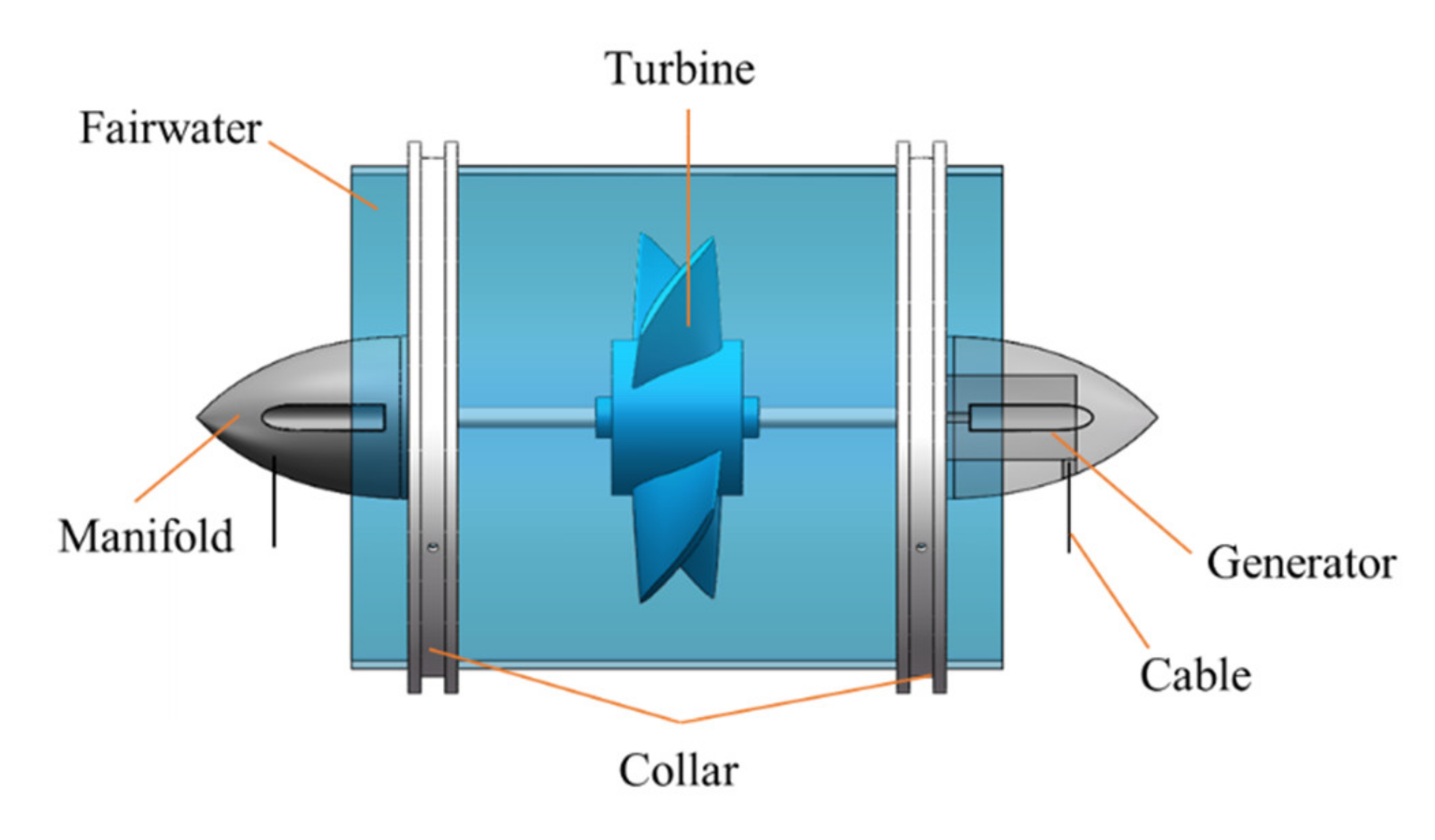
The research in this paper is based on the S-foil bidirectional energy harvesting marine power turbine developed by our research group. The prototype structure is shown in Figure 4. The turbine can work under bidirectional flow to achieve bidirectional energy harvesting. The energy of the combined action of waves and tidal currents in the turbine is always perpendicular to the rotating plane of the turbine. In the design process of the turbine posture change law, calculating the equivalent vector of the wave and tidal current integration energy will make the theoretical design of the turbine posture change law more targeted and convenient.
Furthermore, wave-tidal current coupling is a relatively complex physical process. Therefore, in this paper, the actual working conditions of waves and tidal currents are appropriately idealized, and the complex wave-tidal current coupling process is simplified as a linear superposition mathematical model to integrate the input energy of waves and tidal currents acting on the turbine. This not only fully considers the integration of the two energies but also makes the derivation process simpler.

3.1. Wave Energy

Many existing studies simplify the actual wave condition as a linear wave to calculate wave energy, but the sea conditions in different sea areas are different. It is necessary to determine the applicable wave theory of Lianyungang port according to the values of H / g T 2 and d / g T 2 to calculate the corresponding wave energy [26]. The water depth of Lianyungang port (34.8N, 119.4E) is approximately 14 m according to the China Port Network. Significant wave height, mean wave period, and mean wave direction corresponding to this position were obtained from the ERA5 reanalysis database, and the time resolution is an hour. When significant wave height and the mean wave period of 2018–2021 are introduced into H / g T 2 and d / g T 2 , the obtained values are 0.0037 and 0.0817 respectively, which is in line with the applicable scope of the Stokes second-order nonlinear wave theory. Therefore, the Stokes second-order nonlinear wave theory is taken as the theoretical waveform of Lianyungang port to solve the wave energy. Equations (6)–(11) are the calculation formulas of the solution process [27].
The dispersion relation of the Stokes second-order nonlinear wave is as follows:
L = g T 2 2 π tanh d k
The velocity potential function is as follows:
Φ = π H k T cosh k ( z + d ) sinh k d sin ( k x w t ) + 3 π H 2 16 T cosh 2 k ( z + d ) sinh 4 k d sin 2 ( k x w t )
The wave surface equation is as follows:
η = H 2 cos ( k x w t ) + π H 8 H L cosh k d ( 2 + cosh 2 k d ) sinh 3 k d cos 2 ( k x w t )
The water particle movement velocity components are as follows:
u x = Φ x = π H T cosh k ( z + d ) sinh k d cos Θ + 3 4 π H T π H L cosh 2 k ( z + d ) sinh 4 k d cos 2 Θ
u z = Φ z = = π H T sinh k ( z + d ) sinh k d sin Θ + 3 4 π H T π H L sinh 2 k ( z + d ) sinh 4 k d sin 2 Θ
where Θ = k x w t , d is the water depth (m), H is the wave height (m), T is the wave period (s), L is the wavelength (m), k is the wavenumber, and w is the angular frequency (rad/s).
The energy of horizontal motion of wave particles acting on the turbine in unit wavelength is as follows:
E k = 0 L d η 1 2 ρ ( u x 2 + u z 2 ) d z d x
Equations (6)–(10) can be substituted into Equation (11) to approximate the solution of wave energy using MATLAB software yields:
E k = 1 16 ρ g H 2 + 7 16 ρ π 2 H 3 T 2

3.2. Equivalent Velocities of Waves and Tidal Currents

The tidal current energy calculation equation is as follows:
W = 1 2 ρ v 3 S
where ρ is the seawater density (kg/m3) and S is the flow area (m2).
Since the wave energy does not entirely act on the turbine, the effective wave load acting on the turbine is transformed into the flow load under the same flow area through the equation, and the equivalent flow velocity corresponding to the wave energy is calculated. The wave energy in the unit wavelength is written as the form of tidal current energy:
1 2 ρ v w 3 S = 1 η ( 1 16 ρ g H 2 + 7 16 ρ π 2 H 3 T 2 )
where the coefficient 1 / η represents the proportion of the wave energy actually acting on the turbine. The equivalent tidal current velocity, v w , of wave energy per unit wavelength acting on the turbine is expressed as follows:
v w = 1 8 η S g H 2 + 7 π 2 H 3 T 2 3
The equivalent velocity is superimposed on the tidal current velocity, v t , at this position to obtain the combined velocity, v , of wave-tidal current integration. The vector form of the tidal current velocity and the equivalent velocity of a wave is expressed as follows:
v w = v w v w
v t = v t v t
where v w and v t represent the wave direction angle and tidal current direction angle, respectively.
The velocity vector of wave-tidal current integration is as follows:
v = v w + v t = v w v w + v t v t = v v
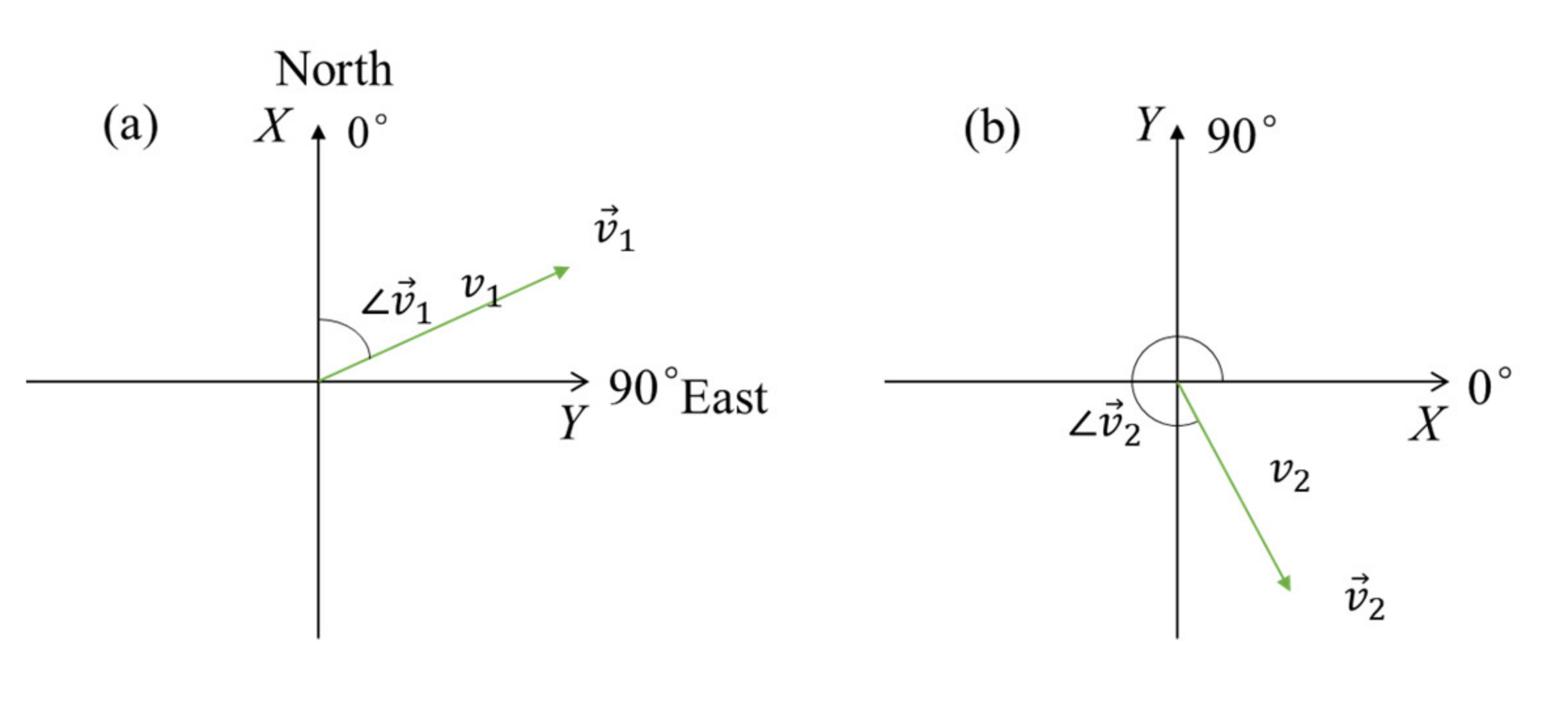
The transformation of the coordinate system between the two-dimensional geographic coordinate system and the mathematical rectangular coordinate system XOY is carried out as shown in Figure 5. In the figure, (a) is the coordinate system of the combined velocity vector integrating waves and tidal currents, and (b) is the mathematical rectangular coordinate system XOY. In the coordinate system in Figure 5a, due north (positive direction of the X axis) is at 0 degrees, and due east (positive direction of the Y axis) is at 90 degrees.
As shown in Figure 5, in coordinate system (a), the vertical axis is the X-axis, the horizontal axis is the Y-axis, and the positive direction of the angle is clockwise. In coordinate system (b), the vertical axis is the Y-axis, the horizontal axis is the X-axis, and the positive direction of the angle is counterclockwise. A vector of angle θ and length l in frame (a) corresponds to a vector of angle 2 π θ and length l in frame (b), and the two vectors are projected with the same sign on the X-axis in their respective coordinates and an opposite sign on the Y-axis.
The velocity vector is substituted into the coordinate transformation relationship, as shown in Figure 6, where v 1 + v 2 = 2 π and v 1 = v 2 . In frame (b), the projection of the velocity vector, v 2 , in the x direction is v x 2 = v 2 cos ( v 2 ) = v 2 cos ( 2 π v 1 ) , and the projection of the velocity vector in the y direction is v y 2 = v 2 sin ( v 2 ) = v 2 sin ( 2 π v 1 ) . Corresponding to frame (a), the projection length of the velocity vector, v 1 , in the x direction is v x 1 = v 1 cos ( 2 π v 1 ) , and the projection length in the y direction is v y 1 = v 1 sin ( 2 π v 1 ) .
According to the above transformation relation, the two velocity vectors of tidal currents and waves are decomposed in the coordinate system (b) as shown in Equation (19):
{ v x 2 = v w 2 cos ( v w 2 ) + v t 2 cos ( v t 2 ) v y 2 = v w 2 sin ( v w 2 ) + v t 2 sin ( v t 2 ) v 2 = v x 2 2 + v y 2 2 v 2 = atan v y 2 v x 2
The combined vector is converted to coordinate system (a) by using the conversion relationship, and the integrated velocity vector in the real geographical coordinate system is obtained as shown in Equation (20):
v 1 = v 2 v 1 = 2 π v 2

3.3. Wave Equivalent Velocity Coefficient

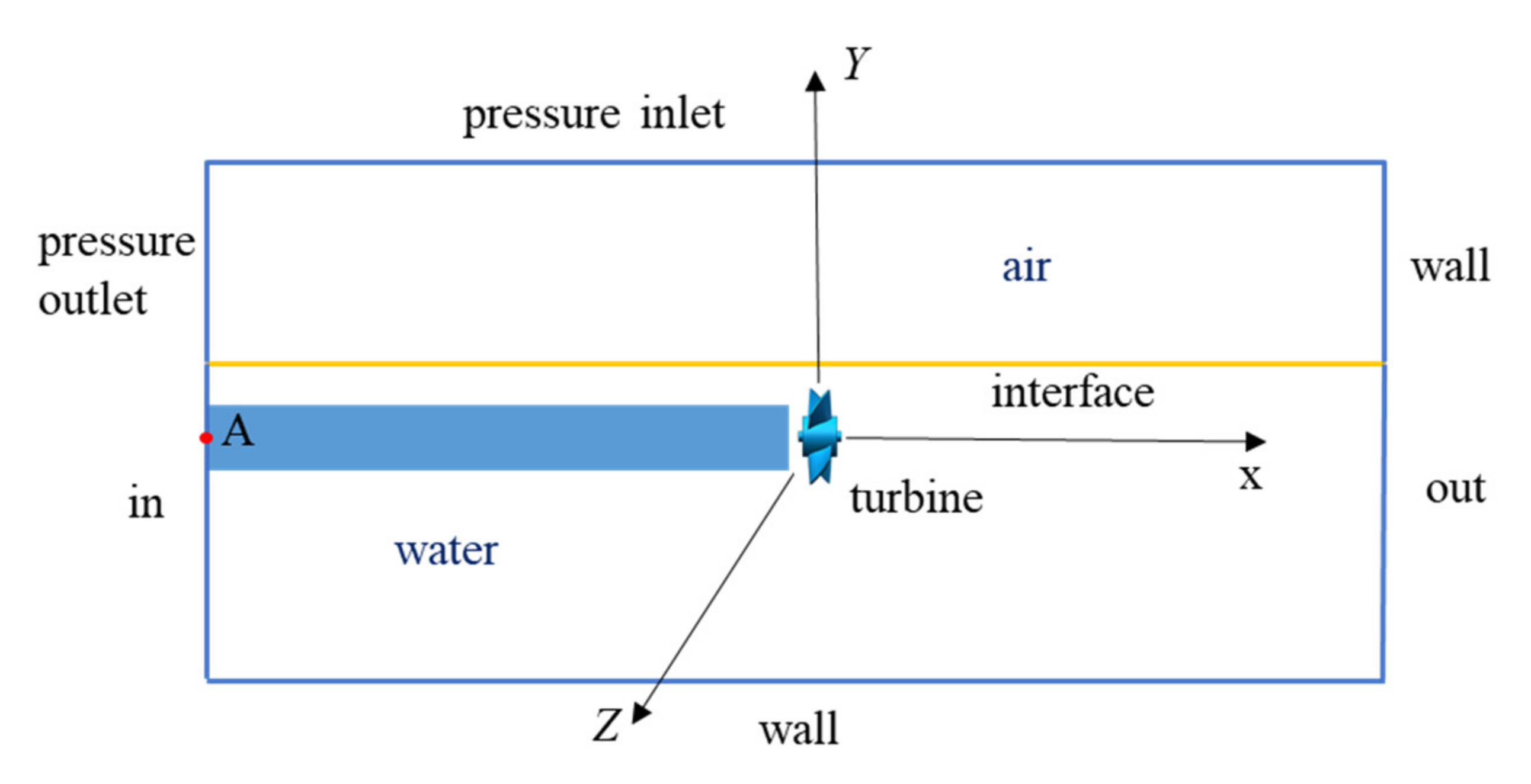
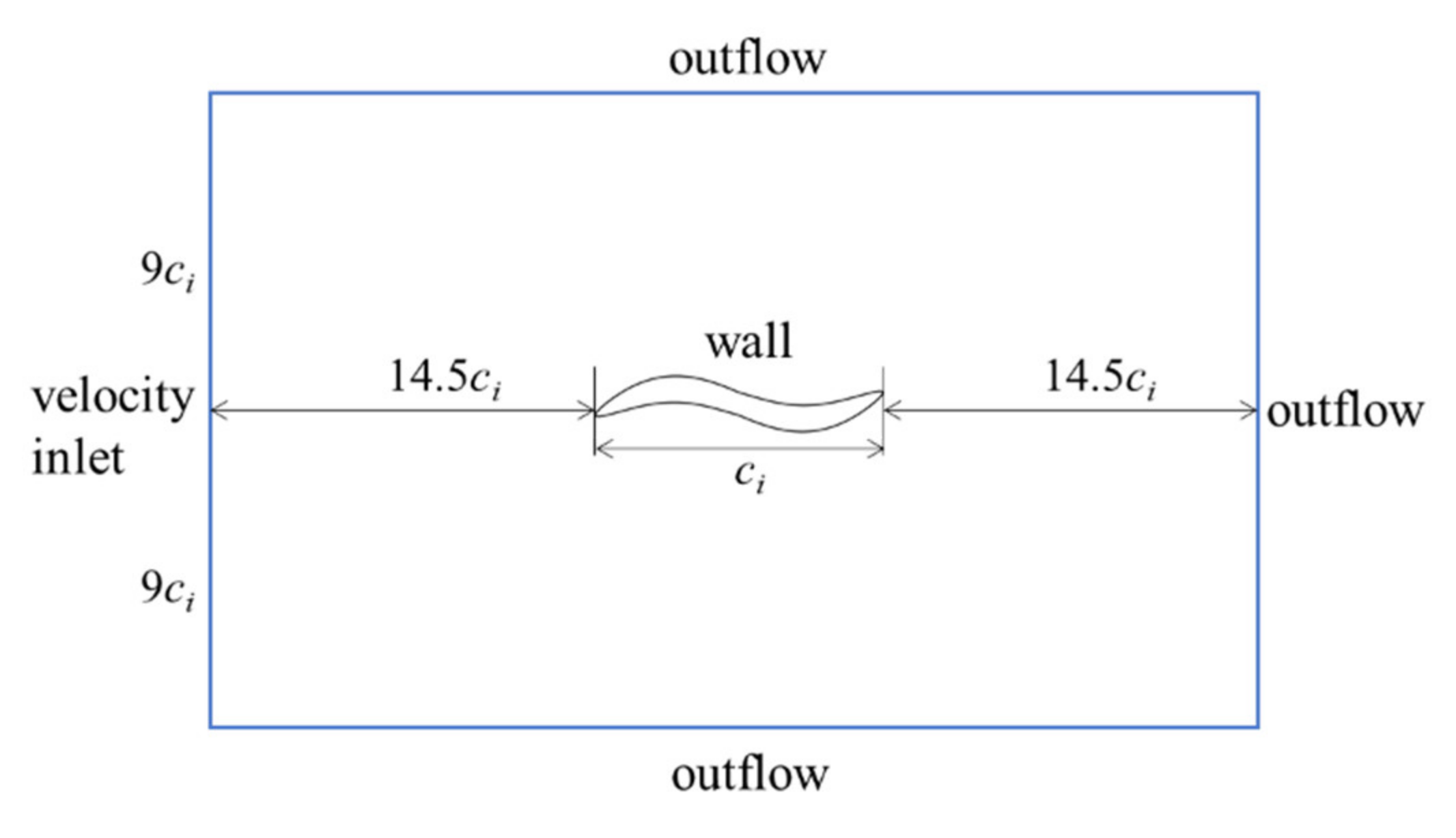
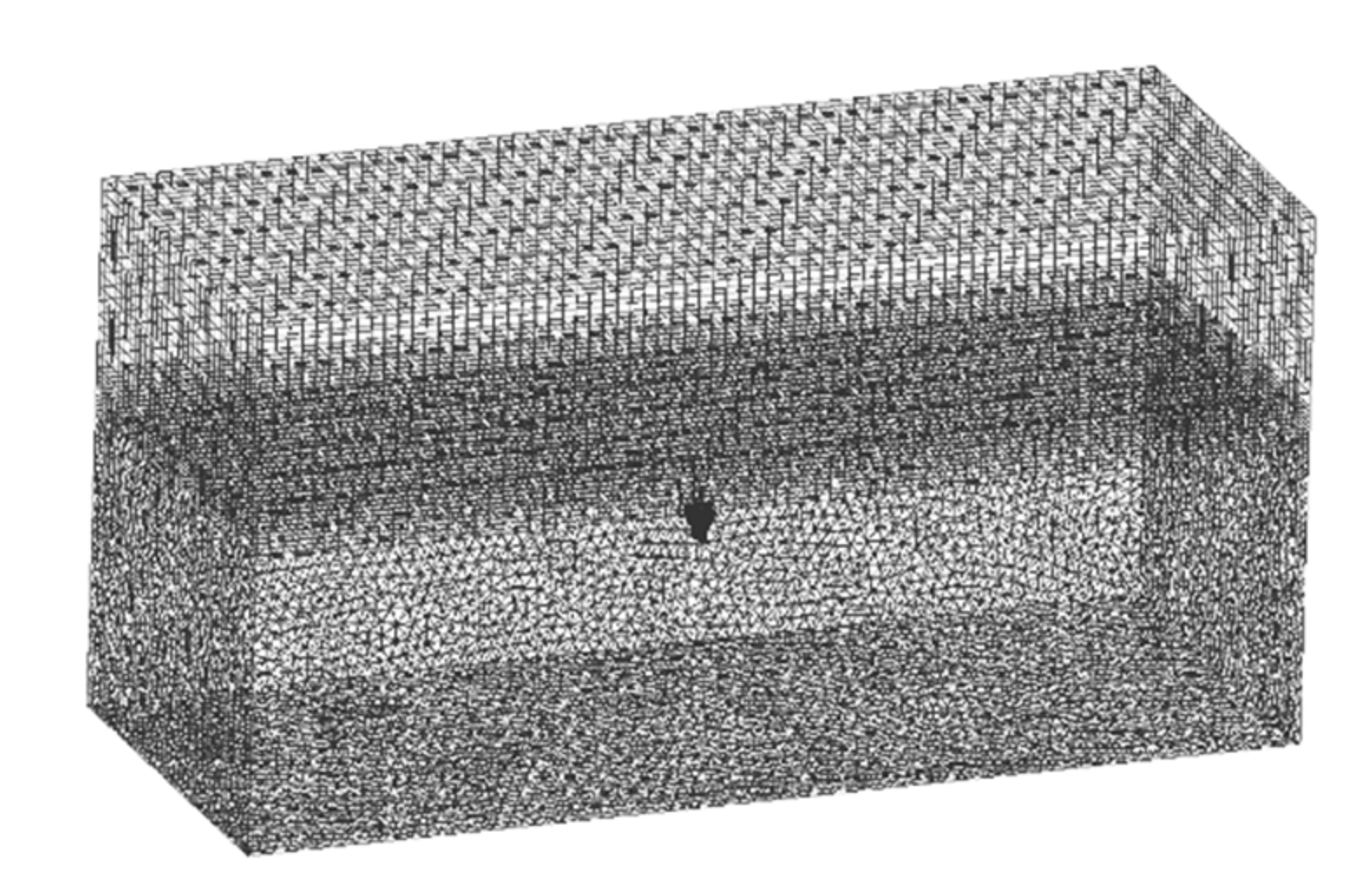
A three-dimensional numerical wave tank was established in Fluent, and its two-dimensional section diagram and boundary conditions are shown in Figure 7. The total grid calculation domain is a rectangular domain with a length of 12D, a width of 6D, and a height of 10D, which is divided into two calculation domains: the air domain and the wave domain. The height ratio of the wave grid calculation domain to the air domain is 3:2. The shape of the air domain is regular compared with that of the wave grid calculation domain. Therefore, the air domain was divided by sweeping grids, and the wave grid calculation domain was divided by tetrahedral grids. When meshing, the size of the turbine wall grid was set to 2.5 mm, the minimum size of the global mesh was set to 0.35 mm, the maximum size of the global surface mesh was set to 35 mm, and the growth rate was set to 1.2. In order to capture the wave propagation of the free surface and the change of wave motion more accurately, the grid was encrypted in a wave height range above and below the static water surface along the wave height direction. The mesh height of the encrypted area was set to 0.1 times that of the wave height, the mesh size in the wavelength direction was set to 0.05 times that of the wavelength, and the mesh size in the width direction of the tank was consistent with the length direction. The total number of grids was 2,108,683, and the Y + value was set to be less than 20. The computational grid model is shown in Figure 8. To calculate the equivalent wave velocity, the Volume of Fluid (VOF) method was used to track the free surface. The Stokes second-order wave was selected. The wave period was set as 0.5 s, the wave height was set as 0.1 m, and the wavenumber was set as 1. According to Equation (6), the wavelength L was obtained as 0.6 m. The Shear Stress Transfer (SST) k-omega turbulence model was chosen, and the pressure-implicit with the splitting of the operator (PISO) algorithm was used as the pressure-velocity coupling algorithm.
The blue part in Figure 7 is the transfer area of wave action. The flow generated by the wave at the starting point was regarded as the equivalent flow of the wave. The velocity of the points in the direction of the Z-axis at point A was calculated in CFD-Post, and the average value was taken as the equivalent flow velocity. The position and velocity of each point are shown in Table 1. The average velocity of each point is 0.34 m/s. The wave energy conversion coefficient, η , can be calculated by Equations (14) and (15) to be approximately 7.48; thus, the coefficient of wave equivalent tidal current velocity can be further deduced.
The wave and tidal current data of Lianyungang port in the past year are substituted to obtain the equivalent velocity range of 0.1–1.2 m/s. Substituting the predicted data of tidal current velocity, tidal current direction, mean wave period, mean wave direction, and significant wave height in Section 2.1 for the next 24 h into Equations (15)–(20), the integrated action velocity vector in the next 24 h can be predicted.
The integration of tidal current energy and wave energy simplifies the effect of complex sea water movement on the turbine into an equivalent velocity vector that varies with time. According to the change in the predicted equivalent velocity size to design the turbine blade motion law, and according to the predicted equivalent velocity direction to design the gesture change law of the turbine, the automatic control system of the blade motion power can be designed according to the obtained law, meaning that the maximum energy acquisition efficiency can be achieved over most of the day.

4. Numerical Analysis of S-foil Turbine Blade Motion

4.1. Theoretical Maximum Energy Acquisition Efficiency

The turbine blade is an S-foil. The symmetry of the S-foil and its optimized hydrodynamic properties give the turbine a good bidirectional flow absorption capacity [28]. The blade section parameters of the prototype designed according to the improved Wilson method [29] are as shown in Table 2.
Due to the reaction to the torque exerted on the turbine by the flow, the flow behind the rotor rotates in the opposite direction, and the rotation of the wake reduces the energy absorption by the turbine. Therefore, considering the rotation of the turbine wake, the axial velocity induction factor, a, and the circumferential velocity induction factor, b [30], are introduced. The stress analysis of the blade element is shown in Figure 9.
The inflow angle, φ , of the blade element is as follows:
tan φ = ( 1 a ) v ( 1 + b ) w r = 1 a 1 + b 1 λ
where v is the inflow velocity (m/s), w is the turbine rotation angular velocity (rad/s), and λ is the tip speed ratio for blade r.
When the system is stably operating, a = 1 3 , b = a ( 1 a ) λ 2 = 2 9 λ 2 . a and b are then substituted into Equation (21):
tan φ = 6 λ t x 9 λ t 2 x 2 + 2
where the design tip speed ratio λ t = w R v and x = r R .
The turbine energy harvesting efficiency can be expressed by its power coefficient (Cp):
C p = 16 9 R λ t x 2 2 3 ξ λ t x + 2 9 λ t x λ t x + 2 9 λ t x ξ + 2 3 d x
where ξ = C L / C D , ξ is the lift-to-drag ratio, C L is the lift coefficient, and C D is the drag coefficient.
The ideal twist angle of the blade element is as follows:
β = φ α b = arctan 6 λ t x 9 λ t 2 x 2 + 2 α b
where α b is the best angle of attack of the blade element, and the lift–drag ratio of the blade element is largest under the best angle of attack, meaning that the turbine energy harvesting efficiency is maximum when the blade is at the best angle of attack [31].
The fluid simulation of the 12 sections of the blade was carried out in Fluent. The range of flow velocity in Lianyungang port was determined to be 0.1–1.2 m/s by the equivalent flow velocity of waves and tidal currents calculated in Section 3.3. Therefore, 12 cross-section airfoils were simulated under the conditions of an attack angle of 0°–18° and an inflow velocity of 0.1–1.2 m/s. Each computational domain of the airfoil was set to a rectangular domain, as shown in Figure 10. The triangular mesh was used for the whole calculation domain. When meshing, the mesh size near the airfoil was set to 0.1 mm. At the same time, in order to encrypt the mesh, it was necessary to add a six-layer expansion line outside the airfoil profile, and the expansion rate was set to be 1.15. The final mesh number was 20,899. The SST k-omega turbulence model was used in the simulation. The inlet boundary was set as the velocity inlet, and the outlet boundary was set as the outflow. The Semi-Implicit Method for Pressure Linked Equation (SIMPLE) algorithm was selected, and the number of iterations was set as 300. When the parameters in the residual curve were lower than 0.001, convergence was achieved. At the same time, the corresponding lift and drag coefficients were monitored, the lift–drag ratio was calculated, and the angle of attack corresponding to the maximum lift–drag ratio was determined. From the simulation calculation, it can be seen that, for different flow velocities, the maximum lift–drag ratios corresponding to the 12 sections are as shown in Figure 11.
The maximum lift–drag ratio curves of each section at different flow velocities in Figure 11 were linearly fitted by a cubic polynomial; namely, ξ = p 1 x 3 + p 2 x 2 + p 3 x + p 4 , where p 1 , p 2 , p 3 , and p 4 are fitting coefficients. The R-square values of the 12 curve fitting equations were greater than 97%, and the fitting effect was good. The 12 curve equations were substituted into Equation (23), and the obtained values are shown in Table 3. It is known that, when the flow velocity is low, the theoretical energy harvesting efficiency of the turbine is low. With increasing flow velocity, the energy harvesting efficiency increases gradually, and the maximum efficiency can reach 29.5%.

4.2. Analysis of Blade Motion under Different Working Conditions

At a flow rate of 0.1−1.2 m/s, the fluid-solid coupling simulation was carried out when the blade twist angles were 10°,12°, 14°, 16°, 18°, 20°, 22°, 24°, 26°, 28°, 30°, 32°, and 34°, and the power coefficients corresponding to each working condition were calculated. The same setting method was used for each working condition of the turbine: the total grid calculation domain was set to the cylindrical domain, and the rotating domain and the outer watershed were established for the turbine. When meshing, the size of the turbine wall grid was set to 1 mm, the size of the grid at the interface between the rotating domain and the outer watershed was set to 4 mm, and the boundary grid of the outer watershed was set to 6 mm. A total of 4,231,110 grids were divided, and the grid quality was checked. The grid with an element quality value between 0.6 and 1 accounted for 87% of the total, which met the calculation requirements. Then, the inlet boundary was set as the velocity inlet, and the outlet boundary was set as the outflow in Fluent. The SST k-omega turbulence model was selected. The PISO algorithm was used for the pressure and velocity coupling algorithm, and the Multiple Reference Frame (MRF) method was used to simulate the turbine. The iterative steps were set to 1500. When the parameters in the residual curve were lower than 0.001, convergence was achieved. The torque coefficients of the turbine were monitored, and the power coefficients were calculated according to Equations (25) and (26). The calculation results are shown in Figure 12.
C m = M 1 2 ρ A R v 2
C p = P o u t P i n = M w 1 2 ρ A v 3
where Pout is the output power (W), Pin is the input power (W), M is the output torque of the rotor (N⋅m), and A is the sweep area of the rotor.
The optimal twist angles and corresponding power coefficients corresponding to each flow condition are shown in Table 4.
Table 4 shows that the power coefficients obtained by the simulation are close to the corresponding theoretical power coefficient. When the inflow velocity is 0.3–0.5 m/s, the energy acquisition efficiency is at its maximum when the turbine blade deflection angle is 26°. When the inflow velocity is 0.6–1.2 m/s, the energy acquisition efficiency is maximal when the turbine blade deflection angle is 20°. The binomial fitting method is used for interpolation between 0.1 and 0.3 m/s, and the twist angle relationship corresponding to the flow velocity is as follows:
θ = 100 v 2 10 v + 20   ( 0.1 < v < 0.3   m / s )
When the inflow velocity is 0.5–0.6 m/s, linear interpolation is used. The relationship between flow velocity and the twist angle is as follows:
θ = 0.7608 v + 0.2196   ( 0.5 < v < 0.6   m / s )

5. Sea Experimental Verification of Wave-Tidal Current Integration

The variable posture law of the hydraulic turbine prototype is verified, and the prototype parameters are shown in Table 5.
The prediction model in Section 2 was used to predict the integrated equivalent flow vector of waves and tidal currents for 19 June 2021. The prediction results are shown in Table 6.
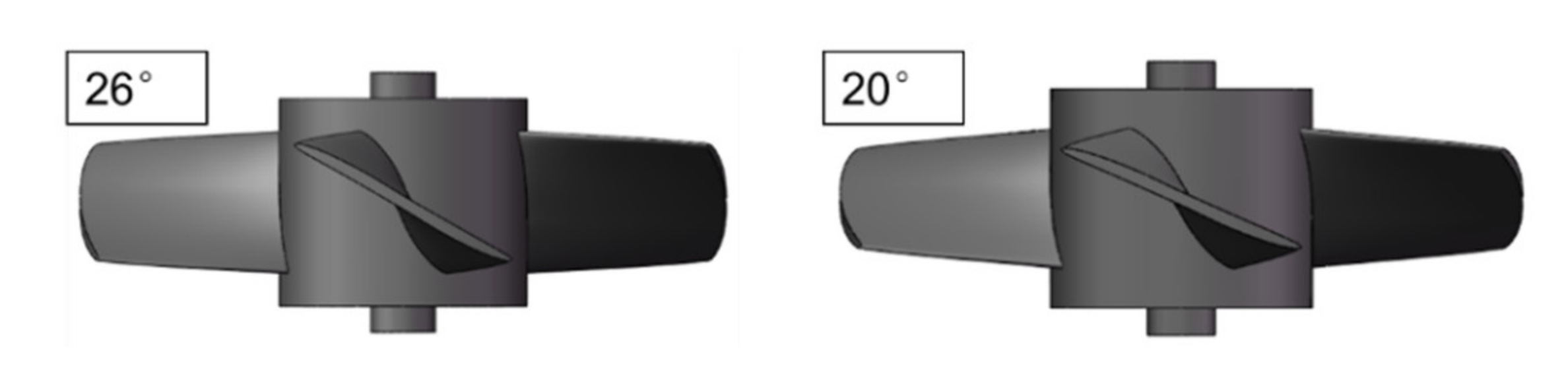
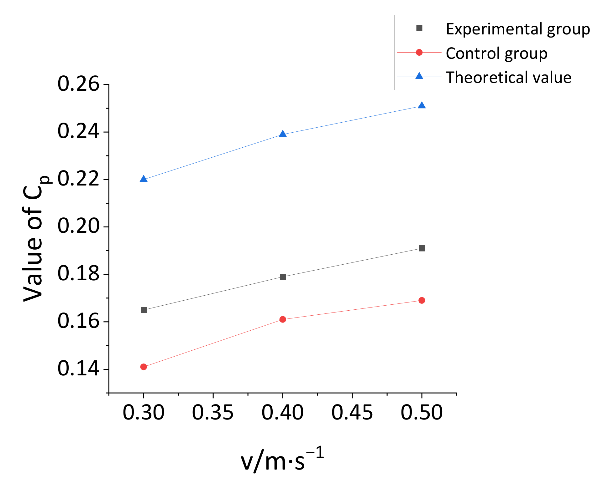
In the two time periods of 10:00–12:00 and 19:00–22:00, the integrated action speed was between 0.3 and 0.5 m/s. In combination with the environmental conditions, these two time periods could be selected for experiments. During the experiment, turbine models with blade twist angles of 26° and 20° were taken as the experimental group and the control group, respectively (Figure 13). The experimental layout and the model sea trial site are shown in Figure 14. The orientation of the device was adjusted according to the integrated action direction at different moments in Table 6. With 60 s as the sampling period, the output voltage and current were collected, and the output power and its average were calculated. The power coefficients were calculated according to Equation (26). The calculation results are shown in Figure 15. The chart shows that when the flow velocity is 0.3–0.5 m/s, the power coefficient of the experimental group (the blade twist angle is 26°) is greater than that of the control group (the blade twist angle is 20°), but it is still less than the theoretical maximum power coefficient. This is because the instability of the flow velocity in the actual sea test resulted in the instability of power generation, but their curve trends are consistent, which is in line with the conclusion of the blade motion law in Section 4.2. Compared with the S-foil wave-tidal current integrated power turbine previously studied by our research team, the blade motion law of the turbine based on the prediction of the wave-tidal current law designed in this paper improves the energy harvesting efficiency of the turbine by about 10% under the same flow conditions.

6. Conclusions

(1) The LSTM neural network prediction model was established for the five parameters (mean wave direction, mean wave period, significant wave height, tidal current velocity, and tidal current direction) of the measured station in the past year, and the data 24 h after the existing data cutoff point were predicted. The results showed that the prediction accuracies of the LSTM neural network model for these five marine parameters were greater than 90%, and the determination coefficients were greater than 90%, indicating that the LSTM model has a good prediction effect for marine parameters. The model can also be further used to predict other marine environmental parameters.
(2) We considered the actual working conditions of the S-foil bidirectional power-harvesting turbine in the process of deducing the mathematical mechanism of wave-current integration. The input energy of waves and tidal currents acting on the turbine was superimposed as an equivalent combined velocity vector. It was deduced that the combined velocity was a function of tidal current velocity, tidal current direction, mean wave period, mean wave direction, and significant wave height. In addition, the equivalent tidal current coefficient of the wave was determined to be 7.48 by using a three-dimensional numerical wave tank. This method not only simplifies the design of blade motion law of a horizontal axis turbine, but also provides a reference for the theoretical derivation of multi-energy integrated power generation.
(3) Through the three-dimensional numerical simulation of the turbine under different working conditions, the blade motion law was obtained. Furthermore, through the sea trial of the prototype turbine, the correctness of the variable posture law of the turbine was verified. When the integrated action speed was 0.3–0.5 m/s, the turbine with a blade torsion angle of 26° was more efficient than the turbine with a blade torsion angle of 20°, which was in line with the design conclusion of the blade motion law in Section 4.2.
(4) The integrated velocity vectors in the next 24 h were predicted by combining the prediction data of five time series and the integrated wave-tidal current action combined vector function. The predicted data were applied to the design of the blade motion law and the rotation law of the turbine fuselage, which could effectively improve the hourly energy acquisition efficiency of the turbine in the working process. Compared with the S-foil wave-tidal current integrated power turbine previously studied by our research team, the blade motion law of the turbine blade based on the prediction of the wave-tidal current law designed in this paper improved the energy efficiency of the turbine by about 10% under the same flow conditions. Therefore, the design method of the blade motion law can provide a reference for improving the efficiency of hydraulic turbines in engineering.
In this study, through theoretical analysis and sea trial experiments, a blade motion law designed based on the prediction of the change law of waves and tidal currents was verified. This experimental method provides a new idea for improving the energy acquisition efficiency of power generation devices. The experimental results can also provide a reference for the engineering design for the development and utilization of new marine energy.

Author Contributions

Conceptualization, Y.L. and S.W.; Formal analysis, Y.L.; Funding acquisition, Y.Z., S.W. and Z.L. (Zhao Liu); Investigation, Y.L.; Methodology, Y.L. and Z.L. (Zeyu Li); Resources, Y.Z., S.W. and Z.L. (Zhao Liu); Software, Y.L.; Validation, Y.L., Z.L. (Zeyu Li) and A.L.; Writing---original draft, Y.L.; Writing---review and editing, Y.L. and Z.L. (Zeyu Li). All authors have read and agreed to the published version of the manuscript.

Funding

This research was funded by the National Natural Science Foundation of China project, grant number 41976194.

Institutional Review Board Statement

Not applicable.

Informed Consent Statement

Not applicable.

Data Availability Statement

Data are contained within the article.

Acknowledgments

The authors wish to thank reviewers who gave valuable suggestion that has helped to improve the quality of the manuscript. The authors also would like to thank editors for the paper revisions and language editing.

Conflicts of Interest

The authors declare no conflict of interest.

References

  1. Wang, S.Q.; Sun, K.; Zhang, J.H.; Zhang, L. The effects of surge motion of the floating platform on hydrodynamics performance of horizontal-axis tidal current turbine. J. Mar. Sci. Technol. 2017, 22, 259–269. [Google Scholar] [CrossRef]
  2. Lv, X.; Guo, P.F. Review of China tidal current energy resource development. Trans. Oceanol. Limnol. 2011, 1, 26–30. [Google Scholar]
  3. Ma, Y.; Ai, S.; Yang, L.; Zhang, A.; Zhou, B. Research on design and optimization of the pitching float wave energy converter. Energy Sci. Eng. 2020, 8, 3866–3882. [Google Scholar] [CrossRef]
  4. Ethan, E.L.; Luksa, L.; Karen, A.F.; Jessica, M.W.; Max, C.V. The influence of surface gravity waves on marine current turbine performance. Int. J. Mar. Energy 2013, 3–4, 27–40. [Google Scholar]
  5. Kuan, L.U.; Wang, H.M.; Han, L.S.; Wen-He, X.U.; Jin, Z.G.; Hui, S.U. Performance Test Research of Tidal Current Energy Convertors Subjected to Wave-Current Interaction. J. Ocean. Technol. 2020, 39, 64–69. [Google Scholar]
  6. Wang, S.; Zhao, F.; Tian, K.; University, S.O. Horizontal wave flow turbine blade optimization analysis based on the theory of orthogonal design. Ocean. Eng. 2016, 34, 109–116. [Google Scholar]
  7. Hedges, T.S. Combinations of waves and currents: An introduction. Proc. Inst. Civil Eng. 1987, 1987.82, 567–585. [Google Scholar] [CrossRef]
  8. Coiro, D.P.; Marco, A.D.; Nicolosi, F.; Melone, S.; Montella, F. Dynamic behaviour of the patented kobold tidal current turbine: Numerical and experimental aspects. Acta Polytech. 2005, 45, 77–84. [Google Scholar] [CrossRef]
  9. Camporeale, S.M.; Magi, V. Streamtube model for analysis of vertical axis variable pitch turbine for marine currents energy conversion. Energy Convers. Manag. 2000, 41, 1811–1827. [Google Scholar] [CrossRef]
  10. Ji, D.H. Research of Wind-Wave Energy Coupling Complementary Genration Platform. Master’s Thesis, Shandong University of Science and Technology, Qingdao, China, 2017. [Google Scholar]
  11. Liu, S.G.; Kai, H.E.; Wan, X.Y.; Qiao, L.; Shang, H.J. A new type of wave, wind and solar integrated power generation ship. Coast. Eng. 2016, 35, 58–62. [Google Scholar]
  12. Lei, D.T. Design and Numerical Simulation Research of Hydro-Turbine Generator Based on Ocean Wave and Current Energy. Master’s Thesis, Shanghai Ocean, University, Shanghai, China, 2014. [Google Scholar]
  13. Ye, L.; Yi, J.H.; Song, H.; Qi, W.; Yang, Z.; Lee, K.S.; Kelley, N.D. On the natural frequency of tidal current power systems—A discussion of sea testing. Appl. Phys. Lett. 2014, 105, 720–2007. [Google Scholar]
  14. Li, B.Y.; Karri, N.; Wang, Q. Three-dimensional numerical analysis on blade response of a vertical-axis tidal current turbine under operational conditions. J. Renew. Sustain. Energy 2014, 6, 435–442. [Google Scholar] [CrossRef] [Green Version]
  15. Chen, J.H.; Wang, X.C.; Li, H.; Jiang, C.H.; Bao, L.J. Design of the blade under low flow velocity for horizontal axis tidal current turbine. J. Mar. Sci. Eng. 2020, 8, 989. [Google Scholar] [CrossRef]
  16. Jun, D.; Zhong, D.S.; Xi, F.W.; Jie, Y. Current research progress of water turbine. Renew. Energy. 2010, 28, 130–133. [Google Scholar]
  17. Chen, Z.; Ma, Y.; Zhang, L.; Su, G.Q. Study on properties of rectangular tidal turbine. J. Huazhong Univ. Sci. Technol. (Nat. Sci. Ed.) 2013, 41, 128–132. [Google Scholar]
  18. Ju, H.L.; Park, S.; Dong, H.K.; Rhee, S.H.; Kim, M.C. Computational methods for performance analysis of horizontal axis tidal stream turbines. Appl. Energy 2012, 98, 512–523. [Google Scholar]
  19. Yong, M.; Liang, Z.; Zhi, Y.Z. Optimization of Blade Motion of Vertical Axis Turbine. China Ocean. Eng. 2016, 30, 140–151. [Google Scholar]
  20. Chen, H.L.; Jing, F.M.; Liu, H.X.; Ding, H.Q.; Shi, J. Numerical and experimental analysis of a vertical-axis eccentric-disc variable-pitch turbine (vevt). China Ocean. Eng. 2020, 34, 411–420. [Google Scholar] [CrossRef]
  21. Bo, J.; Jie, D.; He, W.; Jiang, X.; Qin, Y.; Zhang, J. Wave energy resource assessment along bohai sea, yellow sea and east china sea. Acta Energ. Sol. Sin. 2017, 38, 1711–1716. [Google Scholar]
  22. Mendona, F.; Mostafa, S.S.; Morgado-Dias, F.; Ravelo-García, A.G. On the use of patterns obtained from LSTM and feature-based methods for time series analysis: Application in automatic classification of the cap a phase subtypes. J. Neural Eng. 2021, 18, 036004. [Google Scholar] [CrossRef]
  23. Wang, S.M.; Li, Z.Y.; Li, M.M. Simulation and experimental study based on S airfoil impellers of tidal turbines. Manuf. Autom. 2020, 42, 110–115. [Google Scholar]
  24. Shahid, F.; Zameer, A.; Muneeb, M. A novel genetic LSTM model for wind power forecast. Energy 2021, 223, 120069. [Google Scholar] [CrossRef]
  25. Lei, L.; He, Z.X. Atmospheric Pollutant Prediction Based on Wavelet Decomposition and Long Short-Term Memory Network. In Proceedings of the 3rd International Symposium on Application of Materials Science and Energy Materials (SAMSE 2019), Shanghai, China, 31 December 2019. [Google Scholar]
  26. Gu, D.H. Dynamic Analysis of Structure and Foundation Interaction for Offshore Wind Turbine under Wave Forces. Master’s Thesis, Southeast University, Nanjing, China, 2017. [Google Scholar]
  27. Shan, T.B.; Li, X.; Chen, G.; Xiao, L.F.; Li, J. Leg spacing effect on wave run-up and non-linear wave disturbance along semi-submersible columns. In Proceedings of the 22nd International Offshore and Polar Engineering Conference, International Society of Offshore and Polar Engineers, Rhodes, Greece, 17–23 June 2012. [Google Scholar]
  28. Wei, X.; Huang, B.; Liu, P.; Kanemoto, T.; Wang, L. Experimental investigation into the effects of blade pitch angle and axial distance on the performance of a counter-rotating tidal turbine. Ocean. Eng. 2015, 110, 78–88. [Google Scholar] [CrossRef]
  29. Wang, S.M.; Yang, Z.Q.; Tian, K. Experimental study on the performances of bidirection direct-dirve power turbinf. Ocean. Eng. 2017, 35, 119–124. [Google Scholar] [CrossRef]
  30. Jiang, H.; Yanru, L.I.; Zhao, Y. Torque performance of horizontal axis wind turbines and its impacts of blade tip losses. China Mech. Eng. 2017, 28, 2204–2208. [Google Scholar]
  31. Jiang, H.; Cao, S.; Li, Y. Optimal Twist and Chord of the Blades of Horizontal Axis Wind Turbine. Acta Energ. Sol. Sin. 2013, 34, 1–6. [Google Scholar]
Figure 1. Schematic diagram of recursive structure prediction.
Jmse 09 00869 g001
Figure 2. Model structure of the LSTM network.
Jmse 09 00869 g002
Figure 3. LSTM model prediction results and relative errors: (a) tidal current velocity, (b) tidal current direction, (c) mean wave direction, (d) significant wave height, and (e) mean wave period.
Jmse 09 00869 g003aJmse 09 00869 g003b
Figure 4. Schematic diagram of bidirectional energy-generating turbine.
Jmse 09 00869 g004
Figure 5. Coordinate transformation: (a) two-dimensional geographic coordinate system, (b) mathematical rectangular coordinate system.
Jmse 09 00869 g005
Figure 6. Coordinate transformation of the velocity vector: (a) two-dimensional geographic coordinate system, (b) mathematical rectangular coordinate system.
Jmse 09 00869 g006
Figure 7. Schematic diagram of a two-dimensional section of a numerical wave tank.
Jmse 09 00869 g007
Figure 8. Computational grid model.
Jmse 09 00869 g008
Figure 9. Force analysis of blade element.
Jmse 09 00869 g009
Figure 10. The numerical domain of the airfoil.
Jmse 09 00869 g010
Figure 11. Maximum lift-drag ratio changes of the 12 sections’ blade elements at different velocities.
Jmse 09 00869 g011
Figure 12. Simulation results of hydraulic turbines under different working conditions.
Jmse 09 00869 g012
Figure 13. Experimental hydraulic turbine models.
Jmse 09 00869 g013
Figure 14. Experiment with the prototype turbine in a sea trial.
Jmse 09 00869 g014
Figure 15. Comparison of experimental results.
Jmse 09 00869 g015
Table 1. The equivalent velocities of the wave.
Point Position/mVelocity/m·s−1Point Position/mVelocity/m·s−1
(−2.5, 0, −0.8)0.37(−2.5, 0, 0.2)0.34
(−2.5, 0, −0.6)0.34(−2.5, 0, 0.4)0.31
(−2.5, 0, −0.4)0.33(−2.5, 0, 0.6)0.34
(−2.5, 0, −0.2)0.30(−2.5, 0, 0.8)0.35
(−2.5, 0, 0)0.34--/----/--
Table 2. Parameters of the blade section of the prototype turbine.
Cross-Section i123456789101112
Radius ri/mm4855626976839097104111118125
r/R0.3840.4400.4960.5520.6080.6640.7200.7760.8320.8880.9441
Chord Length ci/mm65.5568.3271.9374.7477.0180.2883.6586.6389.792.7495.0197.28
Twist Angle / β i 28.423.119.517.715.413.2108.35.93.71.50.1
Table 3. Twelve curve fitting results.
v / m s 1 p 1 p 2 p 3 p 4 R - square C p
0.1−4.0835.9121.3796.6250.9890.161
0.26.705−19.2920.783.7030.9970.219
0.323.95−55.8846.36−1.0620.9950.245
0.435.87−80.9563.8−4.3360.9900.259
0.539.09−87.4468.2−4.8830.9930.267
0.645.38−100.777.1−6.440.9910.273
0.752.76−116.588.18−8.5860.9910.279
0.857.57−126.494.8−9.7600.9880.283
0.959.35−131.098.57−10.400.9920.288
1.061.18−135.4102.0−11.080.9940.290
1.167.11−148.0110.5−12.710.9920.292
1.265.90−145.9109.6−12.480.9940.295
Table 4. The optimal twist angles and corresponding power coefficients corresponding to each flow condition.
Velocity/m·s−10.10.20.30.40.50.60.70.80.91.01.11.2
Twist Angle/°202226262620202020202020
Cp0.166 0.191 0.220 0.239 0.251 0.258 0.264 0.270 0.274 0.278 0.282 0.285
Table 5. Turbine prototype parameters.
Turbine Radius (R)125 mmNominal Power40 W
Hub Radius48 mmNominal Velocity2 m/s
Blade Number (B)4Design Cp0.4
Hub Width80 mmDesign λ t 5.5
Sweep Area (S)0.042 m2--/----/--
Table 6. Integrated wave-tidal current results based on predicted data.
Time/h0:001:002:003:004:005:006:007:008:009:0010:0011:00
Integrated Velocity/(m·s−1)1.051.151.161.091.000.910.830.720.650.550.400.18
Integrated Direction/°8370543512346322310295289279287
Time/h12:0013:0014:0015:0016:0017:0018:0019:0020:0021:0022:0023:00
Integrated Velocity/(m·s−1)0.280.560.770.951.020.890.630.360.230.290.370.57
Integrated Direction/°333728181412132562277287280
Publisher’s Note: MDPI stays neutral with regard to jurisdictional claims in published maps and institutional affiliations.

