Article

Design and Analysis of a Mooring System for a Wave Energy Converter

Centre for Marine Technology and Ocean Engineering (CENTEC), Instituto Superior Técnico, Universidade de Lisboa, Av. Rovisco Pais, 1049-001 Lisboa, Portugal
*
Author to whom correspondence should be addressed.
J. Mar. Sci. Eng. 2021, 9(7), 782; https://doi.org/10.3390/jmse9070782
Submission received: 5 July 2021 / Accepted: 14 July 2021 / Published: 19 July 2021
(This article belongs to the Special Issue Hydrodynamics and Mooring Analysis of Floating Structures)

Abstract

:
The objective of this work is to develop an efficient method to carry out the preliminary design of the mooring system for a wave energy converter. A practical mooring design procedure is applied to a specific case of study, and it can be replicated for other cases. Firstly, the static analysis is performed for a configuration with three mooring cables with different pre-tensions on fairlead, diameters of the cables, and materials. Based on these configurations from the static analysis, a quasi-static analysis is carried out in the frequency domain and a preliminary design is conducted according to DNV rules. Then, a 3-h dynamic analysis in the time domain is performed on several selected configurations, considering the same environmental conditions in the quasi-static analysis using the finite element method. Extreme dynamic responses of the system, such as extreme surge motion and mooring tensions, are estimated by the global maximum method, which is performed by fitting 20 individual maximum observations by Gumbel distribution. The quasi-static method is validated by comparing the results of extreme tension and displacement with the coupled time domain analysis. In addition, the influence of pre-tensions and cable diameters on the static and dynamic responses of the mooring system are discussed.

1. Introduction

Wave energy converters are considered one of the most promising clean energy sources in the world of renewable energy. These devices convert the kinetic and potential energy of a sea wave into useful mechanical or electrical energy. The potential of this energy source is extremely wide, but this type of system is relatively recent and most of them are still in the preliminary study phase [1,2]. Compared to nearshore regions, offshore locations present significantly larger amounts of wave energy and free sea space, which could facilitate the deployment of larger numbers of wave energy converters (WECs).
For conventional floating structures, mooring is an important component to assure survivability during extreme sea states. For floating WECs, the mooring design is important, not only for station keeping but also for effective power capture and economic issues. Extensive experiences on mooring designs in the offshore oil and gas industry [3] have provided useful references to mooring system design of WECs; however, a detailed discussion of how existing mooring standards from the oil and gas industry fitted in the application of station-keeping of WECs can be found in [4,5]. The main differences between WECs mooring systems compared to those from other offshore applications are discussed in [6], such as enabling resonance at the dominant wave frequency of target site, installation in shallow water (generally less than 100 m), accounting for PTO characteristics, enabling converters to be densely deployed for a WECs farm, a lower return period and relatively high cost.
As known, there are different types of WECs concerning the working principle, which is also relevant to the mooring design. For the motion-independent devices (e.g., OWC), the mooring design is similar to conventional oil and gas platforms, i.e., the resonant period of mooring should be designed outside the wave period to reduce dynamic loads. On the contrary, for the motion-dependent device, the mooring system needs to be designed to make the resonant period of energy extraction primary modes match the classical wave period of the target site as close as possible [6].
Mooring design procedures for WECs are not very frequent in the literature, however, some useful studies can be found. A static method for preliminary mooring design for WECs was presented in [4] based on statistics of mooring design used for CALM and SALM buoys. With this method, the initial mooring configuration, line properties and mooring pretension can be determined, combining with estimated mean environmental loads. Martinelli et al. [7] presented a detailed procedure to design a mooring system and anchor for SEABREATH (an OWC). The mooring systems assessment for large WECs in Demark were studied in [8,9], where the cost of different mooring systems was coarsely estimated. Mooring and foundation design of marine renewable energy (MRE) devices was performed in [10] using an open-source solution DTOcean (Optimal Design Tools for Ocean Energy Arrays), which is capable of capturing several key aspects of MRE array design and providing the design with lowest capital cost.
A conceptual mooring system design procedure is given in IEC TS 6200-10 [11] considering the ultimate limit states (ULS), the accidental limit states (ALS), serviceability limit states (SLS) and the fatigue limit states (FLS) design. Based on this research, a clear mooring design procedure was proposed in [12]. A review and discussion on the development of the OWC concept of wave energy converters in general and the evolved variation of the Multi-OWC were presented in [13]. Recently, a preliminary design of a floating offshore version of CECO was presented in [14] with two main designs, where the first was a spar solution with the use of catenary mooring (chain) lines while the second design was based on a tension leg platform (TLP) solution with the use of tethers as mooring system. Their analysis on moorings concluded that particular attention should be paid to mooring system design, in terms of properties and materials selection, in order to increase efficiency and at the same time reduce extreme mooring loads and fatigue.
Bergdahl and Kofoed [15] carried out a preliminary design of the mooring system for a WEC, following a quasi-static approach. Chakrabarti [16] published a book that covers the basic background materials and their application in offshore engineering. Particular emphasis is placed on the application of the theory to practical problems. It includes the practical aspects of the offshore structures with handy design guides and simple description of the various components of offshore engineering and their functions. Recently, Ma et al. [3] presented in-depth knowledge on all aspects of mooring systems, from design and analysis to installation, operation, maintenance and integrity management for offshore structures. Xu et al. [17] performed a study on the calculation of the most probable maximum extreme (MPME) responses for floating structure. The global maximum method, which is applied by fitting, using the L-moments method, the individual maximum observations by Gumbel distribution, is used to obtain extreme surge motion and mooring tensions. A slack mooring and two hybrid mooring systems for a WEC buoy were experimentally studied in [18], which showed that the snap load can frequently occur in the slack mooring system. The effects of wave-induced response of floating CALM buoys on the load combination of submarine hose systems and sensitivity studies were performed by Amaechi et al. [19,20] using the hydrodynamic models developed using ANSYS AQWA and the coupled simulation in Orcaflex. An experimental and numerical investigation of a taut-moored wave energy converter system was performed in [21] where the wire ropes were applied in the mooring cables. Yang et al. [22] simulated the dynamics of the WEC system using both coupled and de-coupled models in the time-domain. The coupled approach in DeepC was recommended to be used since the coupling effect was crucial for the fatigue damage analysis of the mooring line.
The use of synthetic fibre ropes in the moorings for floating WECs has resulted in significant improvements in safety, performance and economical aspects, due to the lower submerged mass, a lower cost and the potential to reduce peak loads [23]. The typical synthetic rope used for mooring lines is polyester, aramid, HMPE and nylon. A detailed discussion of the performance of different synthetic ropes in the application for marine renewable energy devices was presented in [24], which concluded that polyester and nylon were considered as the suitable material for compliant mooring systems for WECs. Aiming to improve the knowledge of using elastic mooring lines for floating WECs, experimental study [25] and numerical analysis [26] of two mooring systems for WECs have been performed previously. It was found that the slack system, which contains the polyester component in mooring lines provides significantly lower spectral peaks. A clear characterization of the mechanical behaviours is essential to a reliable and economic mooring design for WECs. A large number of investigations regarding the time-dependent material behaviour of synthetic fibre ropes has been reported, e.g., [27,28,29,30,31]. Thomsen et al. [32] investigates the behaviour of a synthetic mooring system applied to the Floating Power Plant wave energy converter using experiments and a quasi-static analysis based on existing guidelines, showing that the simple method underestimated the tensions. A quasi-static analysis and sensitivity investigation of two different mooring configurations—a single anchor leg mooring (SALM) and a three-legged catenary anchor leg system (CALM)—were presented and compared in [33].
Though extensive synthetic material tests exist in the literature, the numerical simulation of the hydrodynamics of floating body moored with nylon and polyester ropes is still limited, as the material exhibit highly nonlinear and time-dependent load-elongation properties. Recently, Pham et al. [34] suggested a practical procedure to perform numerical dynamic modelling of nylon mooring ropes for a floating wind turbine, considering the empirical dynamic stiffness models that were proposed based on the measurements from [35]. Before performing the numerical dynamic modelling of elastic mooring cables, it is necessary to establish an efficient method for preliminary mooring design from which the mooring configurations with the minimum size of the elastic cables could be designed and be optimized easily.
The objective of the work is to develop a reliable and time-efficient method to perform a preliminary design of the mooring system for a wave energy converter. The procedure is presented by applying this method to a case of study, considering a specific location and floating system. The preliminary design of the mooring system is effectuated considering the extreme environmental conditions, relative to the location under examination, with return periods chosen accordingly to the DNV indications [36]. Firstly, considering different possible mooring configurations a static mooring analysis considering various pre-tensions on fairlead, diameters of the cables and different material of mooring lines, is performed for the WEC buoy. Based on these configurations from the static analysis, a quasi-static analysis is carried out in the frequency domain. In this method, wind and current are considered as steady forces and their loads are calculated using the same approach, and wave loads are calculated for first order waves, including loads from superposed regular wave components in irregular waves and mean wave drift load. A static force-displacement study of the system is carried out, in order to be able to perform a quasi-static analysis, considering the different configurations under examination. At this point, through an iterative method, a preliminary design of the mooring system is carried out, following rules and indications of DNV [36,37]. Moreover, the mean offset, top angle, maximum tensions and surge excursion of the system are estimated and analysed, for each configuration. Then, considering several selected configurations and the same environmental conditions of the quasi-static analysis, this method is validated performing 3 h dynamic analysis in the time domain, using the FEM program, which is implemented in the commercial software SESAM. Extreme dynamic responses of the system, such as extreme surge motion and mooring tensions are estimated with the global maximum method, which is performed by fitting 20 individual maximum observations by Gumbel distribution. The results obtained with the two methods (quasi-static and dynamic analysis) are compared and discussed, and considering the small discrepancy of results the quasi-static method is validated. In addition, the effects of different pre-tensions and cable’s diameters on the static and dynamic responses of the mooring system are discussed.

2. Methods

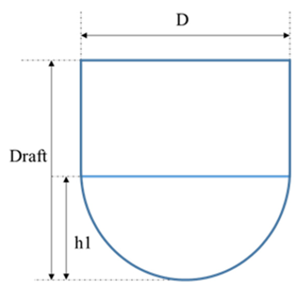
2.1. Description of the Buoy

The water depth (h) of the location under examination is equal to 50 m, while the main characteristics of the WEC are presented in Table 1 and Figure 1. This buoy is a simplified model of a point absorber WEC type and it harvest incoming wave-energy from all directions. This study is mainly focused on the design and analysis of the mooring system.

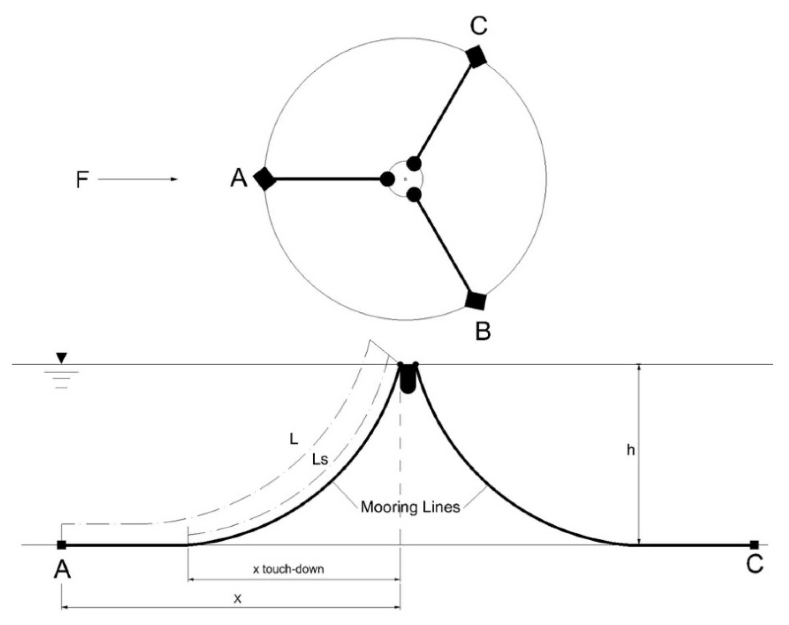
2.2. Quasi-Static Analysis

When a floating structure is exposed to different environmental forces and sea states, the mooring lines are subjected to different types of loads that occur simultaneously:
  • Mean loads;
  • Low frequencies loads;
  • Wave frequencies loads.
Therefore, the mean environmental loads lead the system to a mean horizontal offset (Xmean). In the quasi-static analysis, low frequency and waves loads are computed around this initial offset, considering the stiffness of the mooring system in this position, so that possible resonance effects are taken into account [15]. Then, the larger of the combined horizontal offset (XC) is used to calculate the maximum tension acting on the line:
X C 1 = X m e a n + X W F - m a x + X L F - s i g
X C 2 = X m e a n + X W F - s i g + X L F - m a x
where XC1 and XC2 are the characteristic offset to be considered, XWF-max and XWF-sig are, respectively, the maximum and significant offset caused by wave-frequency loads and XLF-max and XLF-sig are the maximum and significant offset caused by low frequency loads. The index sig and max represent, respectively, the significant and the most probable maximum amplitude motion in three hours [37].
This study is focused on the motion in surge direction and the irregular wave loads are analysed as a superposition of harmonic loads. Solving the equation of motion for the damped system, considering a harmonic load, it is possible to express the horizontal response amplitude ( x ^ ) as [15]:
x ^ = F 0 ( S ( M + M a ) ω 2 ) 2 + b 2 ω 2
where:
  • F0 is the force amplitude;
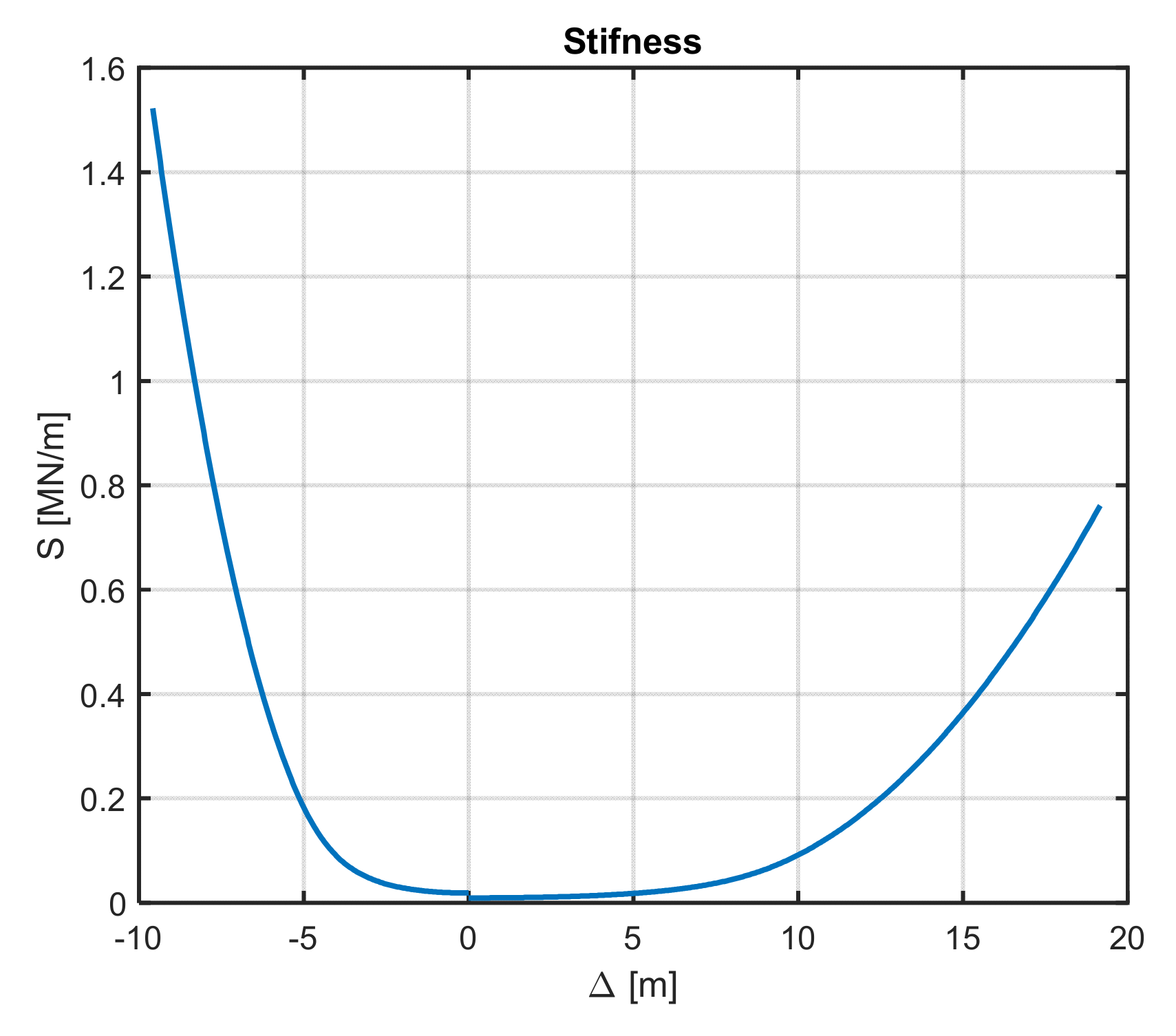
  • S is the mooring stiffness;
  • M is the mass of the floating body and Ma the relative added mass;
  • ω = 2 π T is the angular frequency;
  • b is the radiation damping of the system.
Moreover, the surge motion response spectrum in irregular waves can be calculated using the force spectrum (SF) obtained with the Morison mass force approach (SF) or with the diffraction theory (SFd), but the applied procedure is the same in both cases:
S x ( f ) = S F ( f ) ( S ( M + M a ) ω 2 ) 2 + b 2 ω 2
and the significant motion amplitude:
x 1 s = 2 i S x ( f i ) Δ ( f i )
where Δ ( f i ) is the frequency step ( f i + 1 f i ) .
If the structure’s resonant period is not within the wave spectrum periods (zero up crossing period (TZ) and peak period (TP)), it is possible to apply a simplified equation (Newman approximation) to express the low-frequency excitation spectrum in the frequency domain [38]:
S L F ( τ ) = 8 0 S w ( ω ) S w ( ω + τ ) C d ( ω + τ 2 ) d ω
where S w is the wave spectrum and τ the frequency difference ω i ω j .

2.3. Dynamic Analysis

In the frequency domain analysis, the equations of motions are linearized. Linearity implies some inaccuracy in effects like drag loads, time varying geometry, variable surface elevation and horizontal restoring forces [37]. In addition, the dynamic effects on the moorings are also neglected. To consider the dynamic effects, the moored WEC is modelled and analysed with the software DeepC. This program allows the user to simulate the static and dynamic response of the system, using a time-domain couple analysis approach.
To estimate extreme surge motions and maximum mooring tensions, the global maximum method is applied by fitting 20 individual maximum observations with Gumbel distribution. Using different random seed numbers, it is possible to consider the uncertainty associated with the wave traces and extract uncorrelated and independent maximum values. Usually, at least 20 simulations of 3-h need to be carried out in order to obtain enough values that will produce valid results [17]. Moreover, the extracted maximum values are assumed to satisfy the Gumbel distribution. The cumulative distribution function of this distribution is:
F ( x ; μ , σ ) = exp [ exp ( x μ σ ) ]
where σ is the scale factor and μ is the location factor.
In order to obtain these two factors, the L-moments method is applied, where L-moments are linear combinations of probability weighted moments [39]. The main advantage of this method is that it is robust to possible outliers of the data samples, even for samples with few values. For this reason, it is much more efficient than other traditional techniques, especially for the case under examination, where the size of samples is small and outliers may occur [17]. Therefore, applying this method, the Gumbel parameters are defined as:
  • σ = l 2 ln ( 2 ) ;
  • μ = l 1 γ × σ
where:
  • l 1 = 1 n j = 1 n x j : n , which is the arithmetic mean;
  • l 2 = 2 × 1 n j = 2 n j 1 n 1 l 1 ;
  • γ is the Euler’s constant.
Then, the most probable maximum extreme (MPME) value is calculated as:
x M P = μ σ × ln ( ln ( F ( 1 0.632 ) ) = μ
which is equal to the mode value. This value has a 63.2% chance to be exceeded.

3. Calculations of Environmental Loads

3.1. Environmental Conditions

The environmental conditions considered in the design of a floating device are wind, current and waves. Different return periods should be considered in accordance with DNV rules [36] and with the level of safety required. In this section simple and direct methods are presented to estimate the loads acting on a floating body, generated by varying extreme environmental conditions.
The design location considered in this study is the Arabian Gulf, which is an arm of the Indian Ocean, where nowadays a large number of coastal projects are in progress and many others are being planned for the future [40]. Current velocity (UC) of 1 m/s and significant wave height (HS) equal to 5 m are considered extreme environmental conditions according to [40]. Wind forces are not taken into account in this study, but their loads can be calculated following the same approach presented to estimate the current loads.
A sea state is specified by a wave frequency spectrum with a given significant wave height, a representative frequency, a mean propagation direction and a spreading function. The spectrum provides the distribution of energy among different wave frequency. In applications, the sea state is assumed to be a stationary random process and the standard time between registrations of sea states is usually equal to three hours.
A Pierson–Moskowitz wave spectrum is considered in this study, which is a one parameter spectrum of a fully developed sea. Therefore, the density energy of the spectrum as a function of frequency S w (f), can be calculated from the significant wave height as [41]:
S w ( f ) = 8.10 10 3 g 2 ( 2 π ) 4 f 5 exp [ 0.032 ( g H s ( 2 π f ) 2 ) 2 ]
where g = 9.81 m/s2 is the gravitational acceleration and f the frequency (Hz).
Assuming that the sea state follows a Rayleigh distribution, the 3-h most probable maximum wave can be calculated as [15]:
H m a x = H s 0.5 ln ( N ) = H s 0.5 ln ( 3   h / Tz ) = 1.9   Hs = 9.5   m
where N represent the number of oscillations; considering a 3-h sea state and a zero-crossing mean period (TZ) of 7.9 s; N is approximatively equal to 1300 (N = 3 h/TZ).

3.2. Environmental Loads

3.2.1. Current Load

The current velocity is considered constant for the whole water column, from the mean water level (z = 0 m) to the sea bottom (z = −50 m). The current force acting on a floating structure is found to vary with the square of the flow velocity and as a first approximation, the mean current load can be calculated using the drag force formulation [15]:
F D = C D A 1 2 ρ U 2
where A is the cross-sectional area projected transverse the flow direction, ρ is the density of the fluid, U is the mean of the fluid velocity at the height of the centre of the exposed body and CD is the drag coefficient.
To estimate CD, first it is necessary to calculate the Reynolds number (Re):
R e = U × D v a = 8.4 × 10 6
where:
  • v a is the kinematic viscosity of the fluid ( v a = 1.19 × 10 6   m 2 / s ) ;
  • D is the diameter of the exposed body’s section considered;
  • U is the mean speed of the fluid.
For this Reynolds number and smooth elements (low roughness), DNV [36] gives a drag coefficient (CD) equal to 0.75. When estimating the drag force on a slender member, the integrated sum of sectional force contributions should be multiplied by a reduction factor k. In the case under examination, the aspect ratio 2Db/D is equal to 2.4, where Db is the draught of the body. This gives a reduction factor for finite member k = 0.8 [36]. The seawater density is assumed to equal 1025.9 kg/m3 and the current force acting on the system is then:
F C = k C D A 1 2 ρ U 2 = 33.63   kN

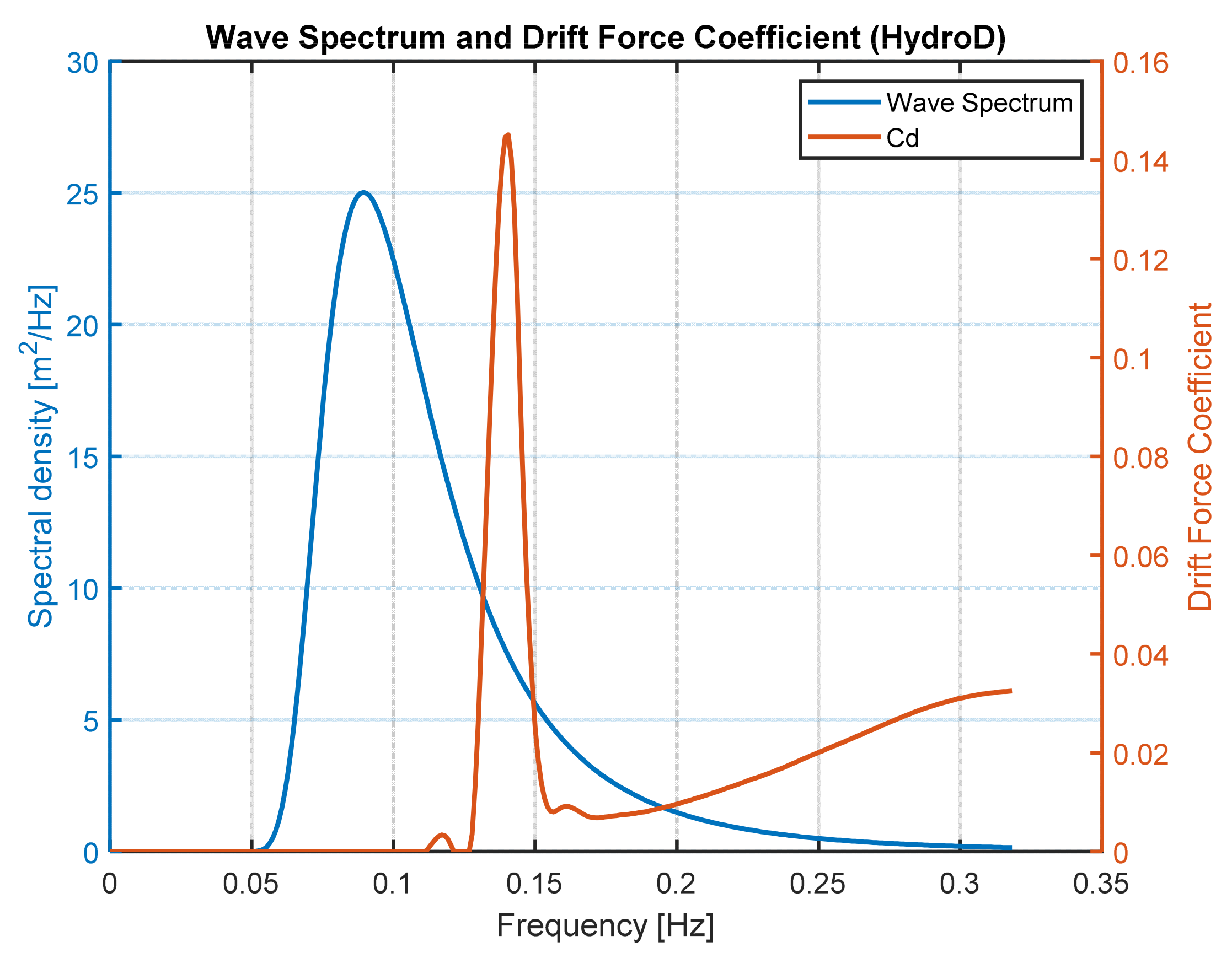
3.2.2. Mean Drift Force

To calculate the mean drift force caused by waves, the simplest and conservative approach is assumed that the object reflects all the incoming waves, with amplitude a i , in the opposite direction of the incoming waves [15]:
F D = 1 2 ρ g 1 2 a i 2 D = ρ g H S 2 32 D = 78.63   kN
However, this method usually overestimates the amplitude of this load, because normally a floating buoy would not reflect wave with wave-length larger than 5 times the diameter. In our case, with deep-water assumption, a wave with a wavelength equal to 5 × D = 50 m corresponds to a wave period of 5.66 s. This means that for wave frequency smaller than 0.18 Hz, the simplified formulation, applied previously, cannot be considered valid anymore.
In order to understand the real contribution of the drift force, the drift force coefficient (Cd) is calculated using a panel diffraction program HydroD. Then, it is possible to integrate the total drift force in the sea state. The P-M spectrum, calculated with Equation (9), together with the drift force coefficient, are reported in Figure 2.
The drift force results equal to 29.69 kN, which is less than half of the force estimated with the previous approximated method.

3.2.3. Regular Waves

For slender structural members, which have cross-sectional dimensions sufficiently small, wave loads can be calculated using Morison’s load formula [36]:
F = ρ V ( 1 + C m ) d u d t + 1 2 C D ρ A | u | u
where F is the reaction force of the mooring system, ρ is the density of the water, V represent the displaced volume, Cm is the added mass coefficient and CD the drag coefficient, A is the cross-section area in the direction perpendicular to the relative velocity, u and du/dt are the undisturbed horizontal water velocity and acceleration in the centre of the body. The coefficients of the Morison equation are generally determined from experiments [42]. With the assumption of circular water motion in deep water, the maximum values are:
u m a x = π H m a x T P ; ( d u a d t ) m a x = g k H m a x = ( 2 π ) 2 T P 2 H m a x
where k is the wave number.
It is usually accepted that the diffraction effect becomes important when the diffraction parameter (πD/λ) is greater than 0.5, where D is the characteristic dimension of the structural member in the plane of the wave and λ is the wavelength [36]. In the case under examination, considering a maximum wave height of 9.5 m and a peak period of 10 s, the diffraction parameter and the Keulegan–Carpenter number are:
π D λ = π D / ( g T P 2 2   π   ) 0.2   and   H m a x D 1
which set the system in the inertia and drag regime [36]. This type of structure with a diameter less than 1/4 to 1/5 of the wavelength, has a small effect on the incident wave and consequently, the diffraction component can be neglected [16,36].
Therefore, considering surge motion and applying the Morison equation to a fixed body, the resultant wave force can be set as a combination of an inertia force F M = ρ V ( 1 + C m ) ( d u a d t ) m a x , which is proportional to the undisturbed relative water acceleration in the centre of displacement, and a drag force F D r a g = 1 2 C D ρ A | u | u , which is proportional to the square of the relative velocity between water and body.
The maximum value of the inertia force is: FM = 3.10 MN, while the drag maximum force value is FDrag = 0.50 MN. However, since the horizontal velocity and acceleration are 90 degrees out of phase, the maximum value of the wave force acting on the system is unaffected by the drag component. Therefore, it can be reduced to [15]:
F = F M = ρ V ( 1 + C m ) ( d u a d t ) m a x = 3.10   MN
where V is the submerged volume of the floating body, Cm can be taken from standard values in DNV-RP-205 [36], which in this case gives Cm = 1 and assuming deep water theory: ( d u a d t ) m a x = 1.86   m / s 2 Equation (16).

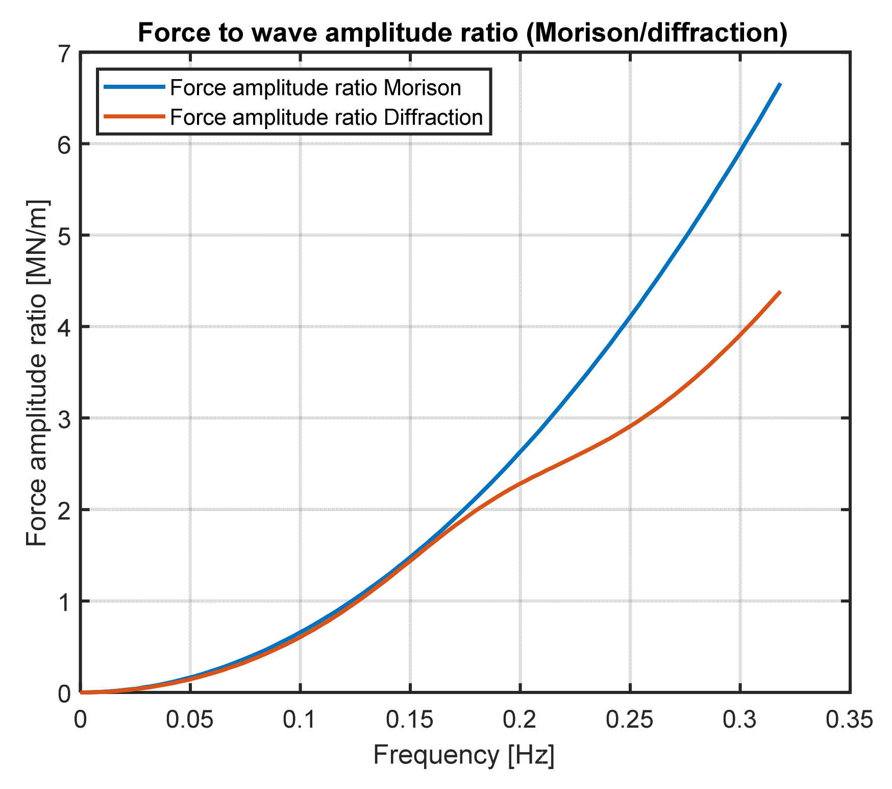
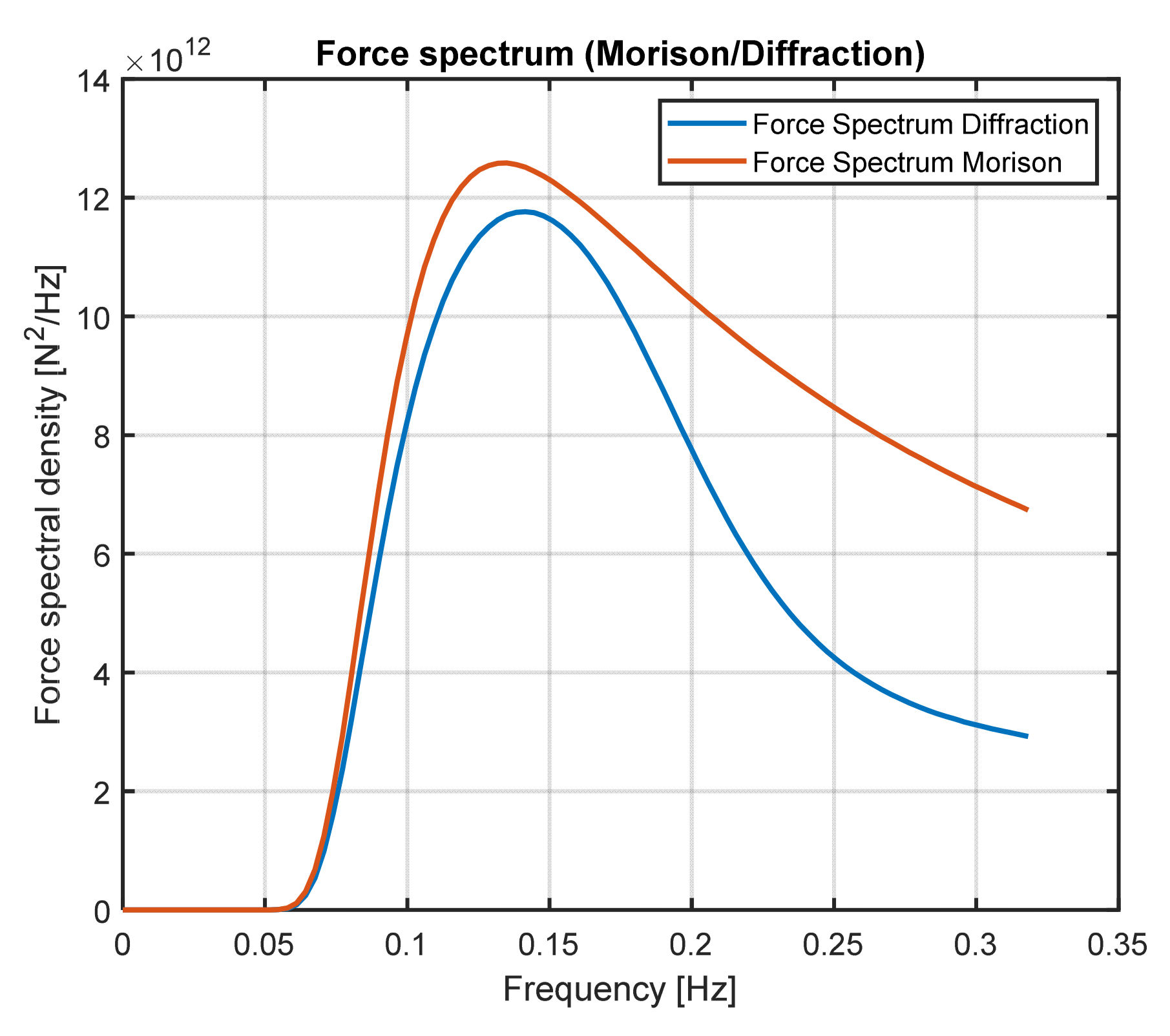
3.2.4. Irregular Waves Morison Approach

The wave force divided by the wave amplitude (a), or wave force amplitude ratio f w ( f ) would become:
f w ( f ) = F a = ρ V a ( 1 + C m ) d u a d t m a x
Then, the wave force spectrum SF(f) can be calculated as:
S F ( f ) = ( f w ( f ) ) 2 × S w ( f )
where the wave spectrum, SW(f), has been defined in Equation (9). The resultant wave force spectrum is reported in Figure 3.
The significant wave force amplitude is then:
F S = 2 S F ( f ) d f = 3.04   MN
Finally, the most probable maximum force can be obtained as:
F m a x = 0.5 ln N × F S = 1.9 × F S = 5.78   MN

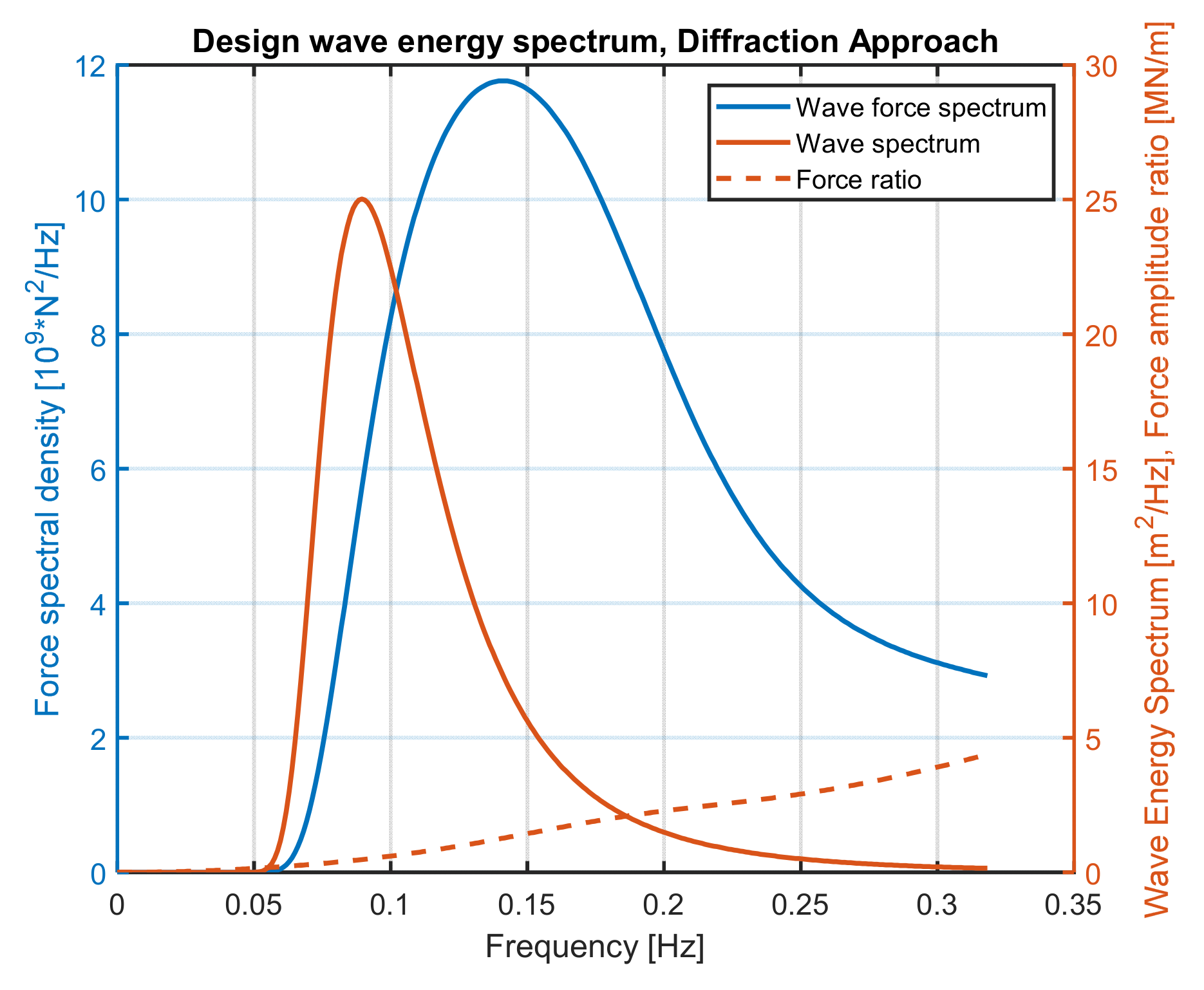
3.2.5. Irregular Waves Diffraction Approach

However, the method presented above presents a limit of accuracy. Indeed, for large structures or relative short waves, when the diffraction parameter ( π D/L) is smaller than 0.5, the Morison equation cannot be considered valid anymore and the wave forces need to be calculated with the linear diffraction theory. Therefore, the body’s hydrodynamic coefficients, radiation damping (b) and added mass (Cm), together with the wave force amplitude ratio (fwd), are calculated as a function of frequency using a panel diffraction program HydroD [43]. The values of added mass and radiation damping, as a function of frequency, are presented in Figure 4 and Figure 5.
At this point, the wave force spectrum can be calculated according to Equation (20) using the diffraction wave amplitude ratio (fwd), which has been calculated by the software HydroD and shown in Figure 6. The results of the wave force spectrums obtained with the two different methods are presented in Figure 7. The diffraction method gives a force reduction of 15% due to the lower force amplitude ratio; the difference can be observed in Figure 8:
As mentioned before, when the diffraction parameter (πD/L) is greater than 0.5 the diffraction theory should be used to compute wave forces. In the case under examination this limit corresponds to a wavelength of 63 m and so, assuming deep water theory, for frequency greater than 0.16 Hz the Morison equation should not be used. Indeed, this limit can be noticed in Figure 8, where for frequency smaller than 0.16 Hz, the force amplitude ratio calculated with the two methods coincides, but for frequency greater than this value the difference is unneglectable, and the Morison approach tends to overestimate the computation.
In order to design the mooring lines considering the most extreme situation that the system will experience, current and waves are assumed to act at the same time and both in the direction of one cable. Considering this assumption, the up-loaded cable is subjected to all the loads acting collinearly in its direction and the design of the mooring cables is based on its dimensions. Table 2 and Table 3 reported the summary on the estimation of mean environmental and wave loads. It can be noticed that the approximated calculation of the wave drift force gives a high overestimated load, for further calculations only the diffraction results are taken into account.

4. Results and Discussions

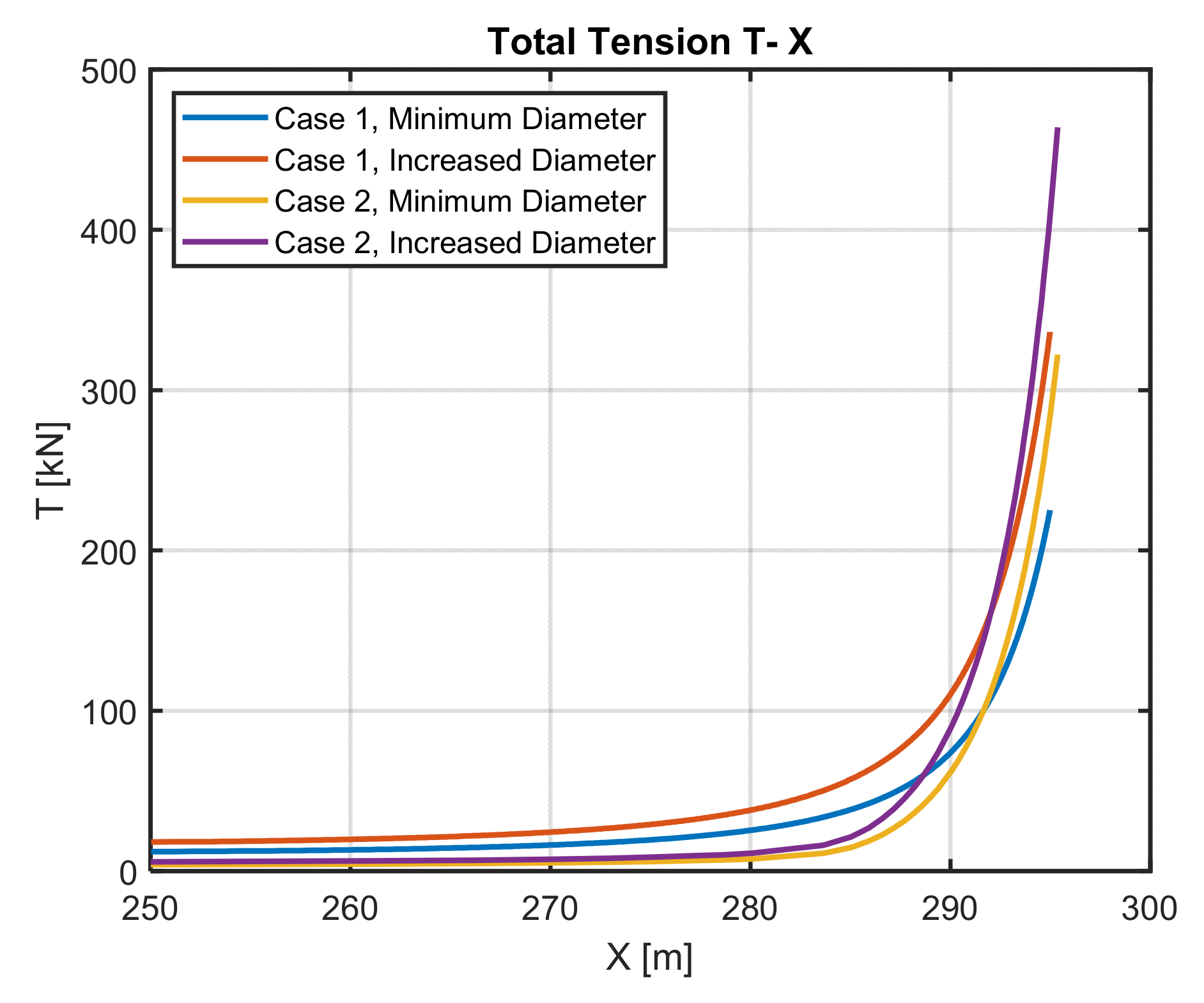
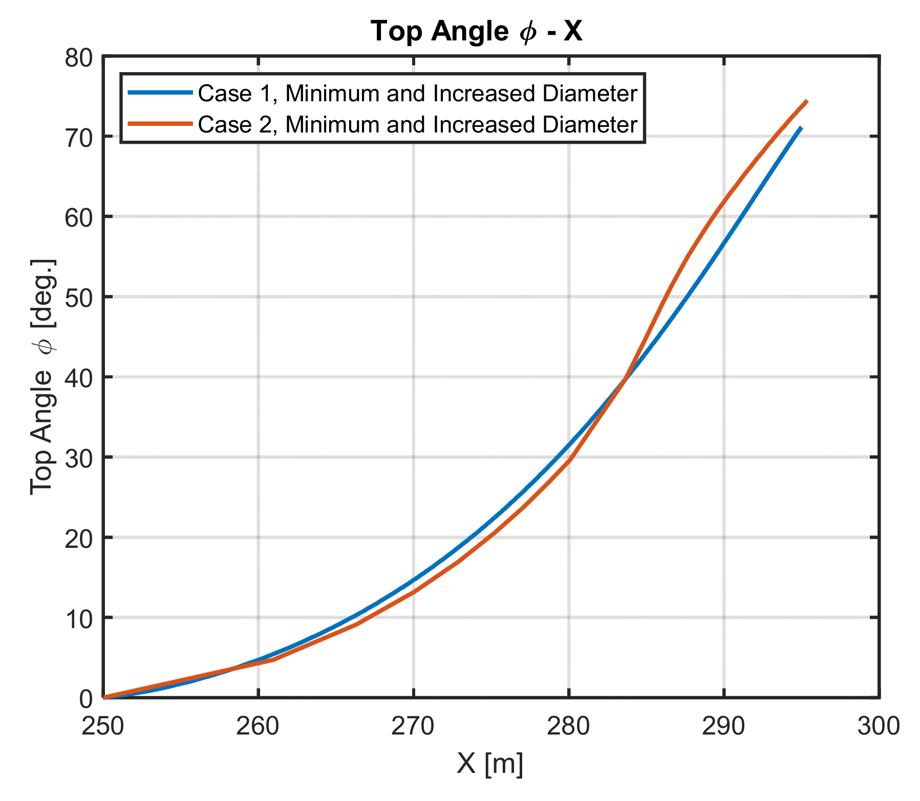
4.1. Quasi-Static Design

A catenary three-legs mooring system with gravity anchors is considered for the WEC, as shown in Figure 9, where F indicates the external force acting on the system and A, B, C are the positions of the gravity anchors. The water depth is equal to 50 m and the total length of each line is L = 300 m. In the study, two mooring systems with different material of the cables are considered and analysed:
Case 1: Catenary, with mooring legs composed by only chain.
Case 2: Catenary, with mooring legs composed of different materials (chain, fibre rope, chain).
The responses of the buoy for both mooring systems are compared varying the pre-tension (TH0) and the diameter of the mooring lines. For both cases, three different pre-tensions (10, 20 and 30 kN) and two diameters of the cable, the minimum that matches the requirements and another one increased by 20%, are applied.
All the configurations are designed in order to satisfy the following requirements:
  • The length of the lifted cable must be lower than the length of the cable (LLift-Max < L).
  • For Case 2, considering that fibre rope is more sensitive to abrasion than the chain, the system has been designed in order to have only the chain laying on the seabed in the initial position [24].
  • The calculated maximum tension (TMax), multiplied by a safety factor (γ) must result in less than 0.95 times the minimum breaking strength (TBR) of the cable, as shown in the following Equation:
T M a x × γ   < 0.95 × T B R
where the safety factor ( γ ) is 1.7 according to DNV rules [36]. Therefore, applying an iterative process until the requirements presented above are fulfilled the material properties chosen for the two mooring systems are summarized in Table 4, Table 5 and Table 6.
Based on these four different configurations, the relation between the vertical tension (TZ), the horizontal tension (TH), the total tension (T) and the top angle (ϕ) on the fairlead with the horizontal distance (X) from the anchor point to the fairlead can be calculated and they are reported in Figure 10, Figure 11, Figure 12 and Figure 13, respectively.
It is observed that in all the cases studied, the tensions increase with the increasing distance from the anchor to the vessel (X). Moreover, for the same system, with a greater diameter, the response behaviours are similar, but with higher values of vertical, horizontal and total tension. This happens because for higher diameters the weight of the line increases. Moreover, it is also found that the three components cable shows almost constant tensions for small horizontal displacements, but between 280 and 290 m, it reaches a point where the tension increases rapidly with small displacements.
Figure 13 shows the relation between the top angle and the horizontal excursion. Unlike tensions, this parameter does not change as the diameter of the lines increases, however, different responses can be observed between Cases 1 and 2.

4.1.1. Initial Position (Zero Offset)

Considering the different pre-tensions (TH0,i) and using the relations between the horizontal tension and the horizontal distances (THX and THx), the horizontal distance from the anchor point to the fairlead (X0) and from the touch-down point to the fairlead (x0) in the equilibrium position, is obtained. Moreover, the static tension in the initial position (T0) is calculated using the relation T = T Z + T H .
Considering the three legs, the total horizontal mooring force as a function of the system’s excursion (Δ) is obtained from the initial offset (X0), in the x-direction, parallel to the upwind leg, where (Δ) is obtained as:
Δ (TH) = X (TH) − X0
Moreover, summing the restoring forces of each cable, total restoring force (FTot) as a function of the vessel’s displacement as calculated as:
F T o t ( Δ ) = T H ( Δ ) 2 cos ( 60 ) T H ( Δ cos ( 60 ) )
Figure 14 presents an example of this calculation, for Case 1 with a pre-tension of 30 kN and the minimum diameter. Figure 15 shows the horizontal stiffness of the mooring system as a function of the horizontal excursion S(Δ), which correspond to the slope of the function presented in Figure 14. It is interesting to notice that the stiffness for the negative excursion is larger than for the positive excursion, which is caused by having two interacting legs in the same direction.

4.1.2. Mean Excursion

Using the mean loads acting on the structure, the mean offset of the structure (Xmean) caused can be calculated. Considering the relation between the horizontal tension and the horizontal excursion (THX), the values of mean offset and the mooring stiffness around it are obtained, for each configuration. The results are summarized in Table 7 and Table 8.
From this results, it can be noticed that by increasing the diameter the mean offset decrease, while the mooring stiffness tends to increase.

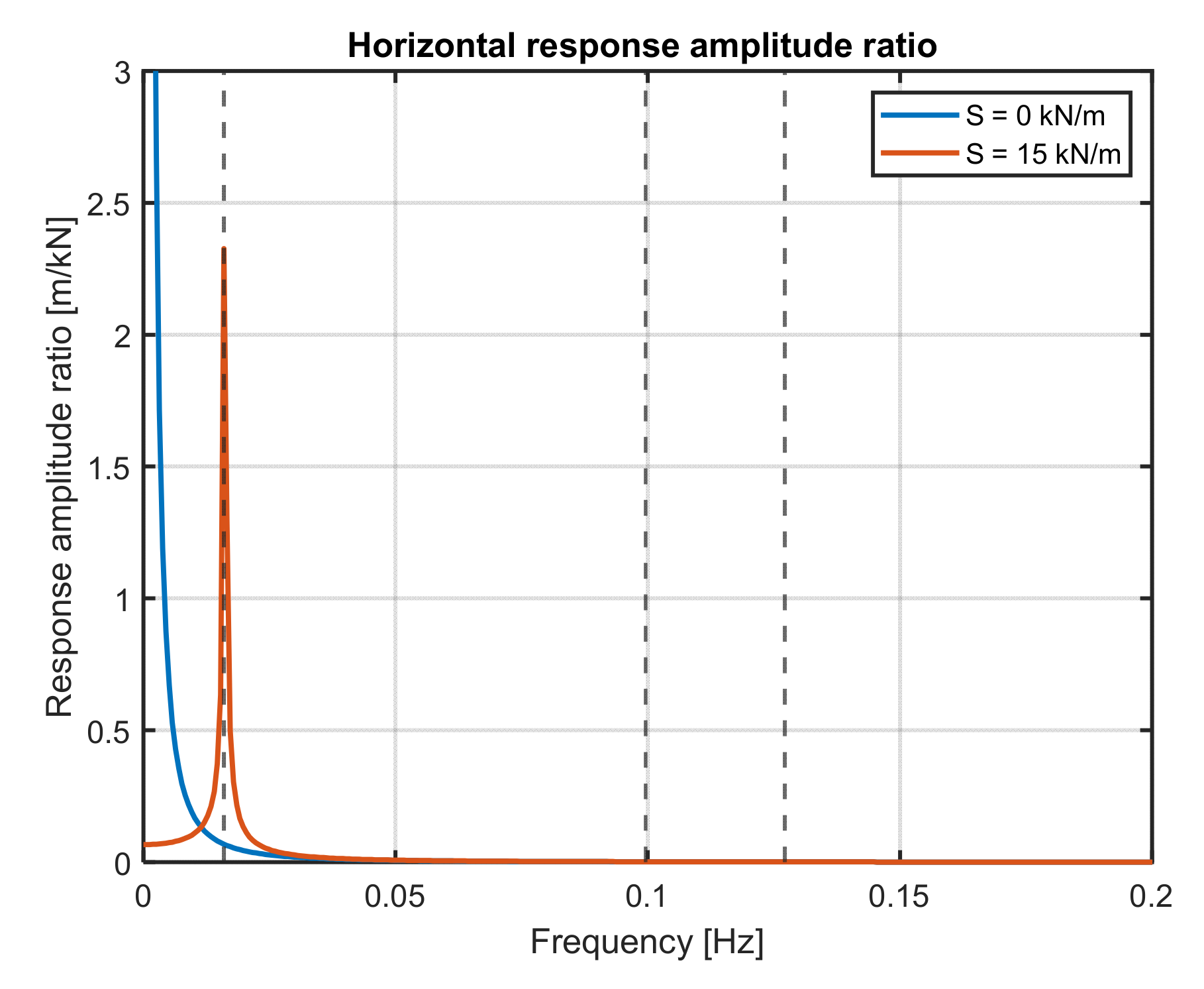
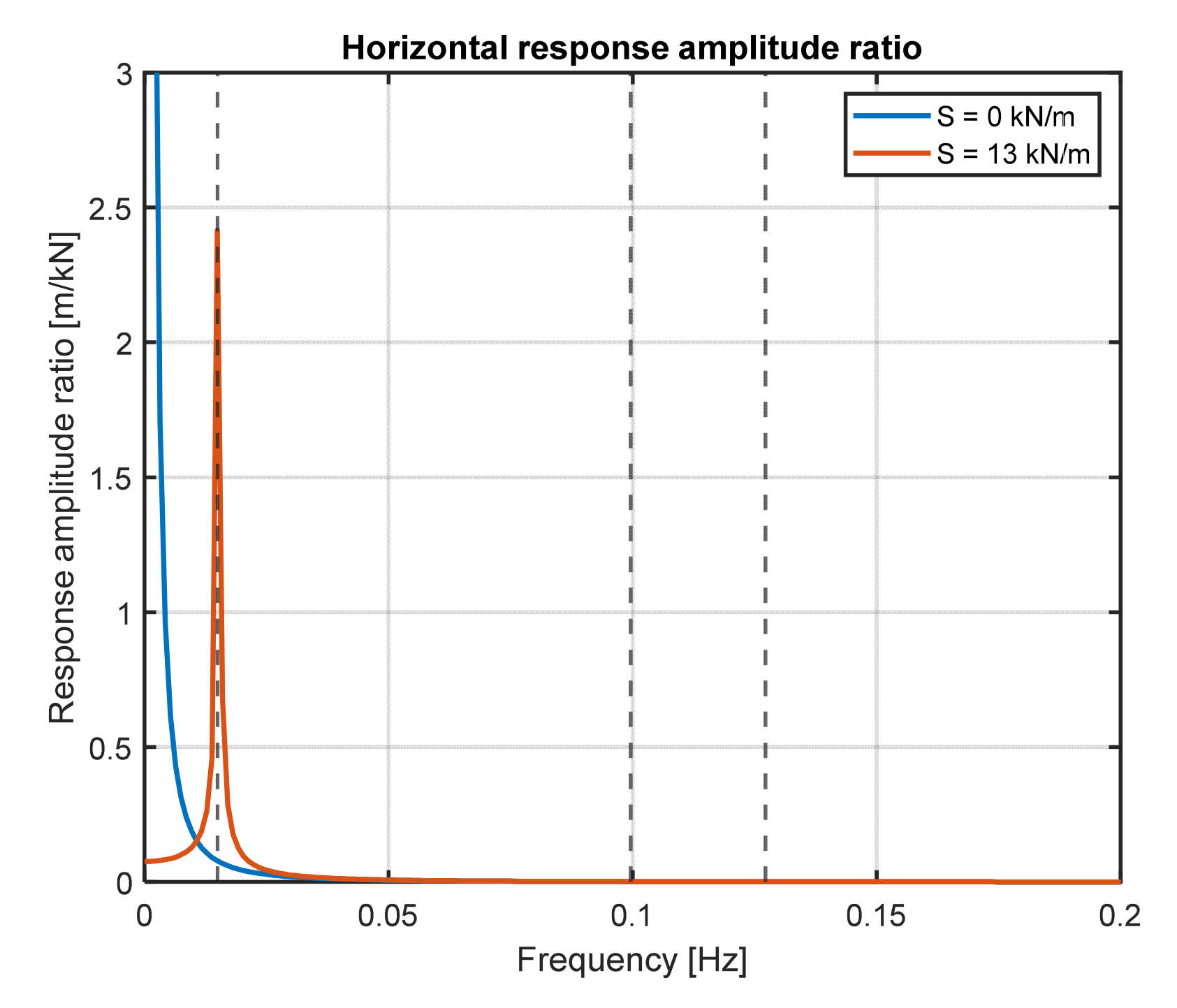
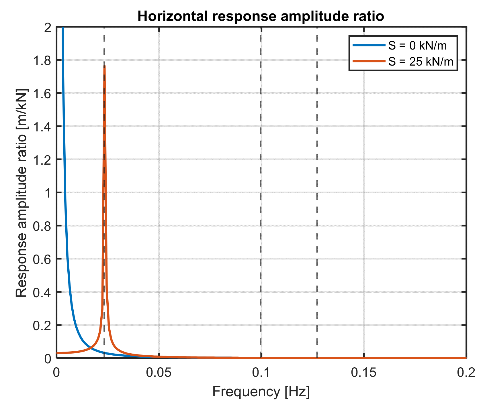
4.1.3. Response Motion to Wave Loads

Considering harmonic loads acting on the structure, the horizontal motion amplitude can be calculated with Equation (3). Three examples of the horizontal response amplitude ratio as a function of frequency are shown in Figure 16, Figure 17 and Figure 18, among all the possible configuration exanimated in this study (Case 1, minimum diameter, pre-tensions of 10 and 30 kN, and Case 2, minimum diameters and pre-tension of 30 kN). The response amplitude ratio is calculated by dividing the surge motion amplitude, obtained with Equation (3), by the wave force F0 = 3.04 MN, which was calculated previously.
Moreover, in these graphs, the surge natural frequencies (different for each configuration), the peak periods (TP) and the zero up crossing periods (TZ), are marked out with dotted lines. In all the figures, it can be seen that the response amplitude has its peak in correspondence with the natural frequency, which underlines the importance of considering possible resonance effects in the system design. In this case, the peak and zero up crossing periods are far enough from the natural frequency to make unlikely possible resonance effects. Moreover, in the same figures, the response of an unmoored system is plotted as well, which have stiffness (S) and natural frequency equal to zero. As expected, it can be noticed that in this case the response diverges for a frequency equal to zero.
As mentioned before, the surge motion response spectrum in irregular waves can be calculated with Equation (4), while Equation (5) gives the significant motion amplitude. Finally, the relative probable maximum excursion in 3-h can be calculated as:
x m a x = 1.9 × x 1 s
where x1s is the significant motion amplitude and has been defined in Equation (5).
Moreover, the wave force spectrum (SF(f)) can be calculated with the Morison mass approach or with the diffraction theory. Consequently, different significant and maximum motion amplitudes are obtained, depending on which method is considered. The results obtained with these two approaches for each configuration are reported in Table 9, Table 10, Table 11 and Table 12. For further calculations and final design of the diameter of the cables, only the diffraction results will be considered since they are obtained with a more accurate method.
From Table 9, Table 10, Table 11 and Table 12, it can be seen that the surge amplitude motion induced by waves, is almost unaffected by the variation of pre-tension and diameter of the cables. This happens because for a small difference of these two parameters, the stiffness does not vary significantly, consequently the wave induced motion does not present a significant change. However, it is important to point out that the pre-tension and the diameter of the cable have an important influence on the calculation of the mean offset and so also on the total maximum surge excursion. Moreover, from the tables present above, it is found that the Morison approach tends to overestimate the wave response amplitude of about 10% compared to the diffraction approach. In the cases under examination, since the drift force coefficient is particularly small and the resonance period is off the peak of the drift force spectrum, the low frequency motion can be neglected as the first approximation and they will not be considered.

4.1.4. Quasi-Static Analysis Results

Considering the mean offset (Xmean) and the maximum excursion caused by wave loads calculated with the diffraction theory, (XWF-Max,D), the maximum horizontal offset of the system from the initial position is estimated as X C = X m e a n + X W F - M a x , D , using the total distance from the anchor (XTOT) and the maximum tension acting on the mooring lines (TMax). Moreover, in order to fulfil the requirements reported previously, it is necessary to verify that the maximum length of the lifted cable is smaller than the length of the cable (LLift-Max < L) and that the utilization factor (u) is lower than 1, where u is expressed as:
u = T M a x × γ   0.95 × T B R < 1
where γ is the safety factor ( γ = 1.7 [36]) and TBR is the breaking strength of the cables.
In the following Table 13, Table 14, Table 15 and Table 16, all the results obtained for each configuration are reported. The results were obtained with an iterative method until the requirements mentioned above were achieved.
The results for Case 1 and minimum diameter are presented in Table 13. In this case, the utilization factor (u) is widely below 1 and the diameter was increased until the value of the length of the maximum lifted cable results smaller than the length of the cable. The results of Case 2 and minimum diameter are reported in Table 15. In this case, the requirements were achieved with more iterations, since all the diameters can be modified. As mentioned before, in order to avoid abrasion of the fibre rope component, in the initial position only the first section of the line (chain) should lay on the sea bottom. Moreover, the utilization factor (u) is close to 1 and at the same time, the maximum lifted cable is close to the length of the cable. It means that the design is not over-dimensioned and consequently, is cost-effective.
Finally, the results for Case 1 and Case 2, with the increased diameter, are summarized in Table 14, Table 15 and Table 16, respectively. In these cases, no iterations are needed, since considering the same force input and increasing the diameters, the length of the suspended cable decreases, as the utilization factor. Analysing the results obtained from the quasi-static analysis, the effects of different pre-tension and diameter of the cable, on the response of the system, are investigated. These effects are summarized in Table 17.
As seen in Table 17, a higher pre-tension would ensure a higher control on the platform’s horizontal displacement, but at the same time, the lines would be subjected to higher tensions. This happens because the length of the suspended line increases and consequently the gravity load generated from the lines, which characterize the catenary systems, also increases. It is also observed that incrementing the diameter and the weight of the cable, the length of the suspended line reduces together with the maximum tension of the mooring system. Moreover, the total distance from the anchor to the vessel reduces, but at the same time the horizontal excursion from the initial position (Xmean), due to mean loads, together with the maximum horizontal excursion (XC) increases. For this reason, an increment of diameter not always leads to a better configuration, not only because of the cost of the material and installation, but also particular attention should be given to the maximum offset limitations of the project under consideration.

4.2. Dynamic Analysis

Three configurations within all the cases presented and analysed in the quasi-static analysis, are considered, and evaluated with static and dynamic coupled analysis through the software DeepC [44]:
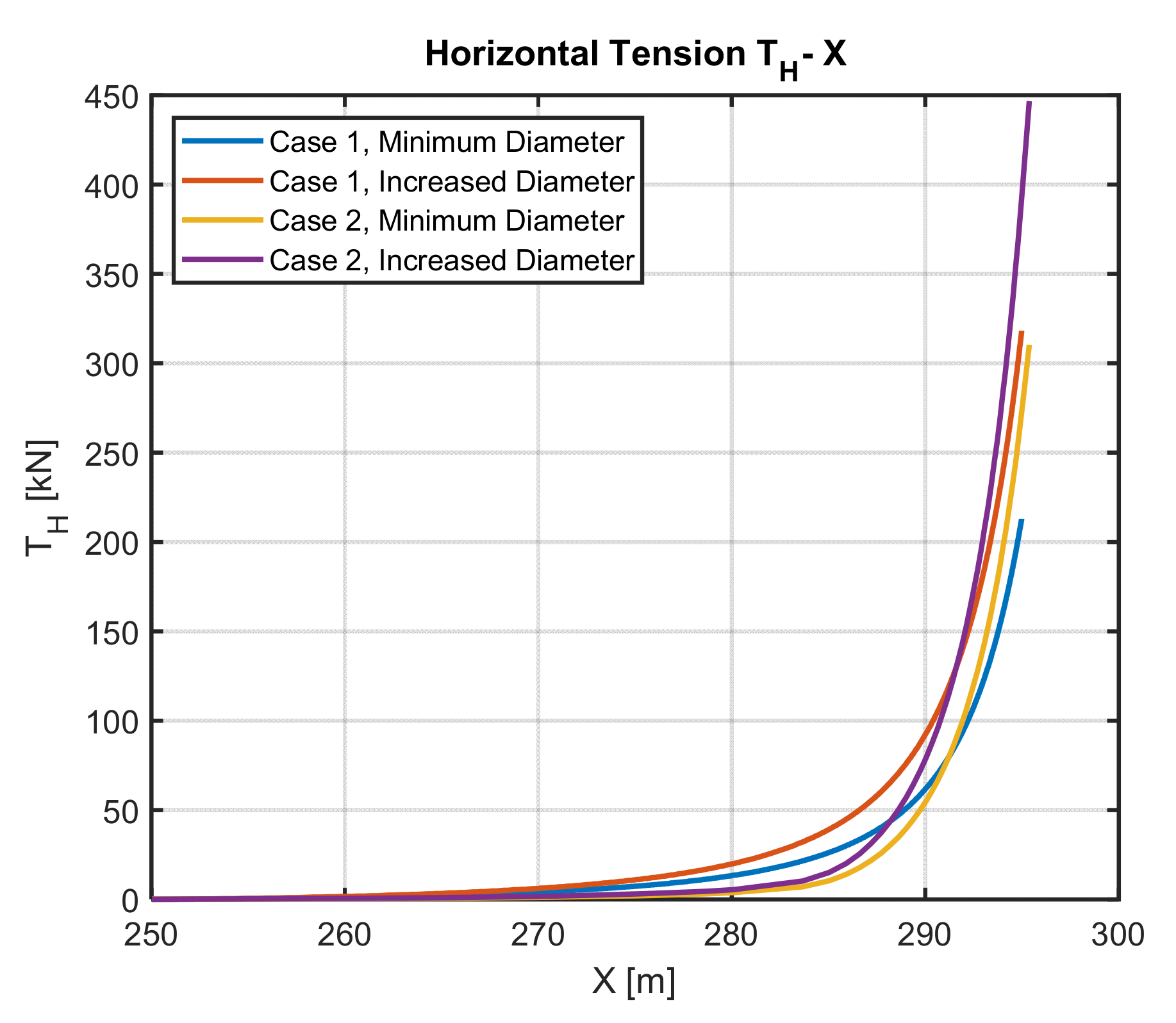
  • Case 1, pre-tension = 30 kN, minimum diameter: D = 36 mm;
  • Case 2, pre-tension = 10 kN; minimum diameter: D = 26 mm, 100 mm, 45 mm;
  • Case 2, pre-tension = 30 kN; minimum diameter: D = 26 mm, 100 mm, 45 mm.
The moored WEC is modelled are represented in Figure 19 with the same dimensions and properties of the buoy analysed in the quasi-static analysis (Table 1 and Figure 1). Both static and 3-h dynamic coupled analysis are performed. More in particular, for each case, considering different random seed numbers ranging from 0 to 100, 20 different dynamic simulations of 3-h are conducted. Then, only the maximum surge amplitude response, together with the maximum tensions acting on the three fairleads, are extracted from each simulation.

4.2.1. Validation

First, by performing a static analysis in DeepC, the values of tension in the initial position (T0) are compared in Table 18 with the values obtained in the quasi-static analysis.
As expected, in the initial position with no external forces acting on the system, the tension calculated by DeepC shows almost identical results of the quasi-static analysis. More in particular, the horizontal mooring force (TH) is equal along the cable and the vertical component (TZ), which depends on the weight of the cable, increases from the bottom to the surface. For this reason, the maximum value of the total tension, which is composed of these two components ( T = T z 2 + T H 2 ), is found to act on the fairlead, that is the top end of the mooring line. Moreover, the quasi-static analysis carried out previously has estimated these values with high accuracy, since for all the cases, the difference is below 3%.

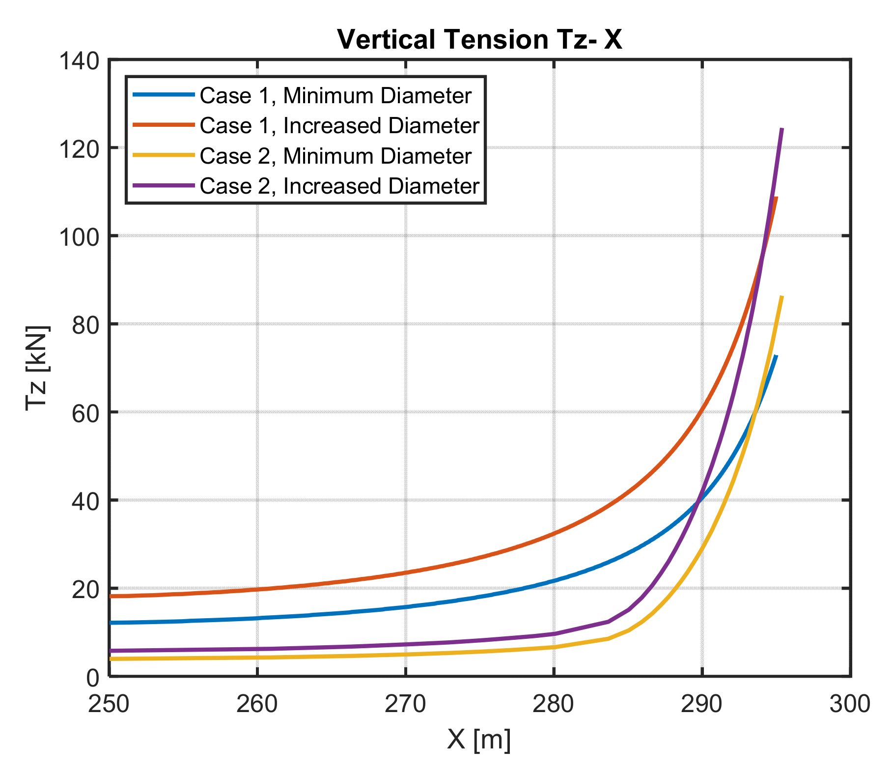
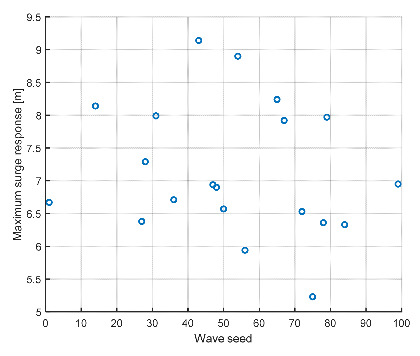
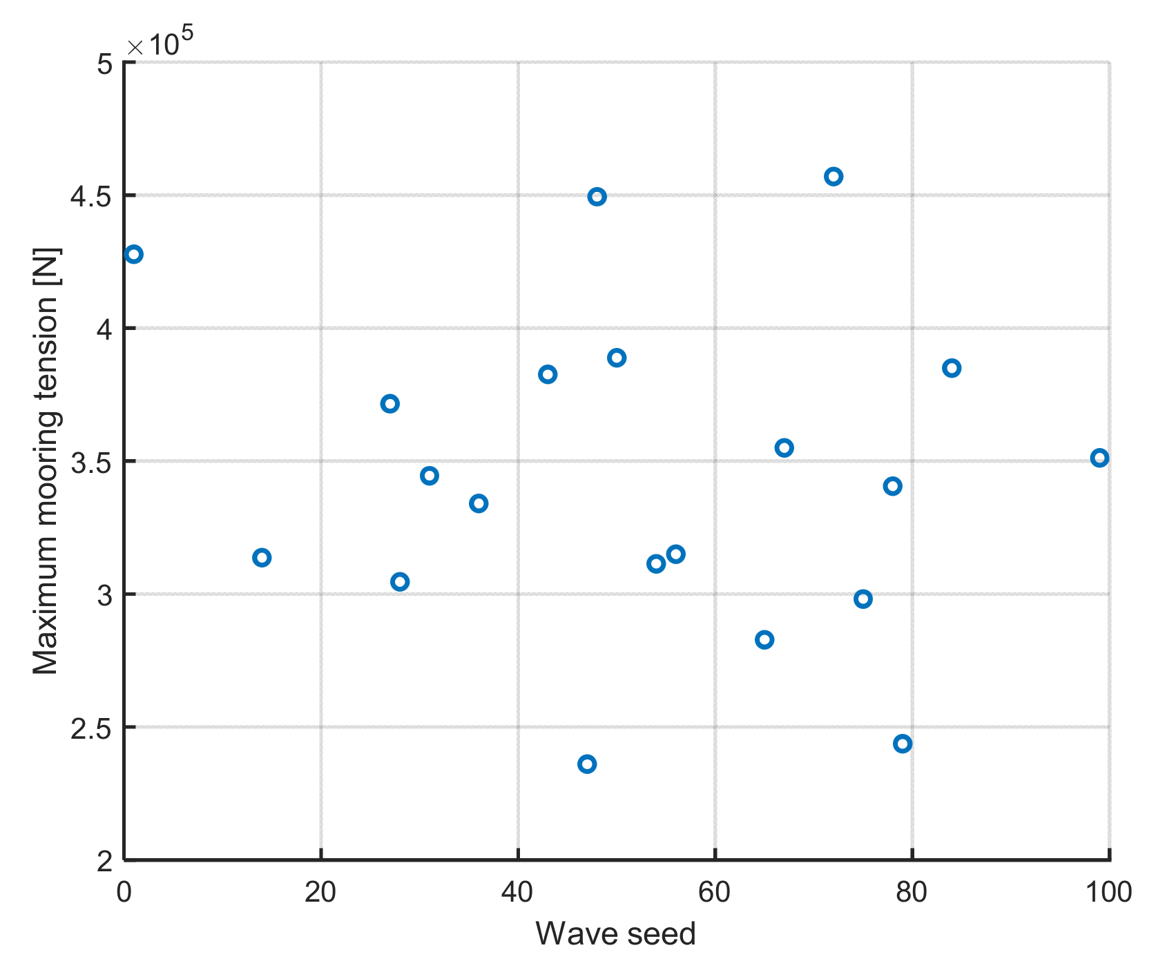
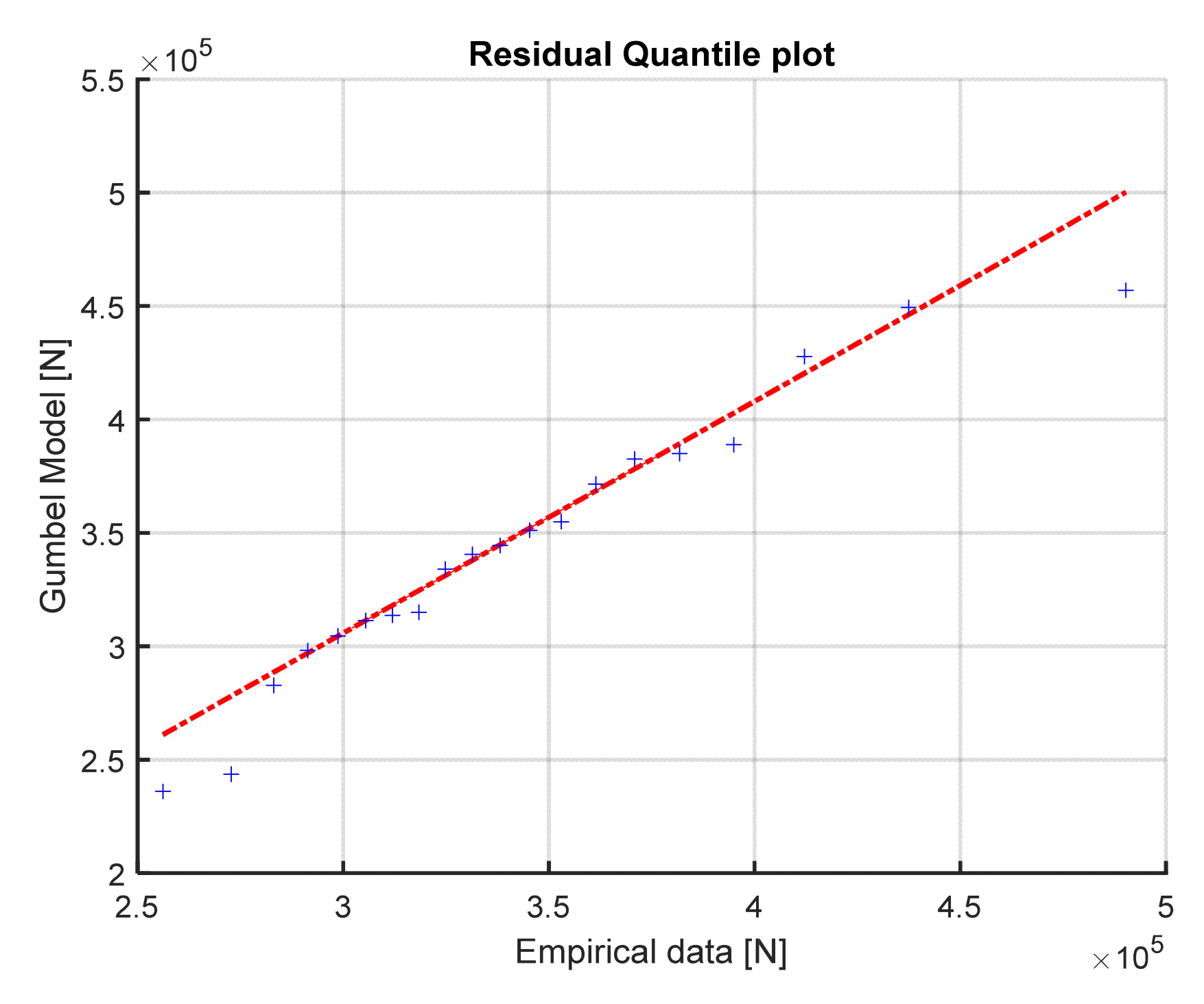
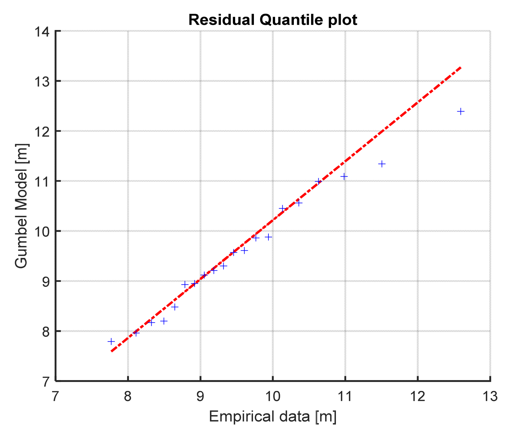
4.2.2. Extreme Values from Dynamic Analysis

After validating the static analysis results, 20 time-domain dynamic analysis of 3-h are performed for each case. The results of maximum tension and surge motion amplitude, vary significantly with the seed number, as can be seen in the examples reported in Figure 20 and Figure 21. This proves that the system dynamic responses are sensitive to the wave train.
The maximum values extracted from each simulation are fitted to the Gumbel distribution Equation (7), estimating the distribution parameters (σ and μ) with the L-moments method. Moreover, to evaluate the accuracy of fitted Gumbel distribution, two examples of the quantiles of the sample data versus the theoretical quantile values from a normal distribution are plotted in Figure 22 and Figure 23. It can be observed that most points distribute along the reference line despite some discrepancy of tail points. This indicates that the estimated Gumbel distribution matches well with empirical data.
Next, the most probable maximum extreme (MPME) value of tension and horizontal motion of the system is calculated based on Equation (8) and compared with the quasi-static analysis results in Table 19, Table 20 and Table 21. In order to consider the worst scenario, the loads are assumed to act collinearly in the direction of one cable. The results of the most probable extreme tensions, calculated with the 3-h coupled analysis (Table 19), show, as expected, higher tensions in the cable parallel to the direction of the environmental forces. More in particular, the up-loads line, presents tensions between 7 to 20% higher than the other two cables, which display a symmetrical behaviour.
Table 20 presents the results of maximum mooring tension, obtained with the two different methods (quasi-static and dynamic analysis). The dynamic time-domain simulations estimate higher values of maximum tension. However, the difference never exceeds 30%, which means that in this case, also the quasi-static analysis provides a good indication of the response of the system. The results of the maximum horizontal excursion are compared in Table 21. It is found that the two different analysis provide similar results in the estimation of the maximum surge excursion, where the higher difference is about 7%.

5. Conclusions

In the study, the quasi-static analysis in the frequency domain and the dynamic analysis in the time domain are performed for a WEC with different mooring configurations. The loads considered in the quasi-static analysis are calculated with two different approaches: the Morison equation and the diffraction theory approach. Different configurations are analysed considering different materials and dimensions of the mooring cable, and pre-tensions, in order to understand the influence of these parameters on the response of the system. Finally, three different configurations are modelled and analysed in the software DeepC.
The comparison between the quasi-static and the coupled dynamic analysis shows almost equal tensions results in the equilibrium position. Moreover, the differences between the maximum excursion of the buoy, from the equilibrium position, calculated with the two different methods (quasi-static and dynamic analysis), are 0.5 to 7%. However, quasi-static analysis tends to underestimate the maximum tensions experimented from the mooring system, which in the coupled analysis are between 5 up to 30% higher. These results show that the approximated quasi-static analysis carried out in this study provides good indications on the extreme values of surge excursion and tensions, but in order to get precise results, a more accurate and time-demanding coupled analysis should be performed.
Comparing the two different configurations evaluated in this study, it is possible to notice that in Case 2, where lines are composed of different materials (chain and synthetic fibre rope), the requirements can be matched varying more of the lines’ parameters than Case 1. Consequently, it is possible to make a more accurate and cost-effective design, considering the different cost of the cables’ materials.
However, unlike rigid lines, synthetic materials such as fibre ropes present highly nonlinear load-elongation characteristics. For this reason, when these types of materials are considered in the design, a coupled dynamic time-domain analysis should be always performed, in order to consider and analyse such nonlinear behaviours. In this study, only the surge motion is considered. To better understand and have a complete view of the behaviour of the system, the other degrees of motion should be analysed as well. Depending on the type of WEC, the heave component can have an important and significant effect on the efficiency of the system. Finally, more configurations, considering different cable’s length and materials, such as wire rope, can be studied and analysed in order to be able to choose the best mooring system among more possible configurations.

Author Contributions

Conceptualization, S.W., S.X. and C.G.S.; methodology, F.D., S.W. and S.X.; software, F.D.; validation, F.D., S.W. and S.X.; formal analysis, F.D.; investigation, F.D., S.W. and S.X.; resources, F.D.; data curation, F.D.; writing—original draft preparation, F.D.; writing—review and editing, F.D., S.W., S.X. and C.G.S.; visualization, F.D.; supervision, S.W., S.X. and C.G.S.; project administration, C.G.S.; funding acquisition, C.G.S. All authors have read and agreed to the published version of the manuscript.

Funding

This work was financially supported by the Project “ELASTMOOR—Elastic mooring systems for wave energy converters”, which is co-funded by European Union’s Horizon 2020 research and innovation programme under the framework of OCEANERA-NET (http://oceaneranet.eu accessed on 5 July 2021) and by the Portuguese Foundation for Science and Technology (Fundação para a Ciência e Tecnologia—FCT) under contract (OCEANERA/0006/2016). The work contributes to the Strategic Research Plan of the Centre for Marine Technology and Ocean Engineering (CENTEC), which is financed by FCT under contract UIDB/UIDP/00134/2020.

Institutional Review Board Statement

Not applicable.

Informed Consent Statement

Not applicable.

Data Availability Statement

Not applicable.

Conflicts of Interest

The authors declare no conflict of interest.

References

  1. Cruz, J. Ocean Wave Energy: Current Status and Future Perspectives; Springer Science & Business Media: Berlin/Heidelberg, Germany, 2007. [Google Scholar]
  2. Czech, B.; Bauer, P. Wave energy converter concepts: Design challenges and classification. IEEE Ind. Electron. Mag. 2012, 6, 4–16. [Google Scholar] [CrossRef]
  3. Guedes Soares, C.; Bhattacharjee, J.; Tello, M.; Pietra, L. Review and Classification of Wave Energy Converters. In Maritime Engineering and Technology; Guedes Soares, C., Garbatov, Y., Sutulo, S., Santos, T.A., Eds.; Taylor & Francis Group: London, UK, 2012; pp. 585–594. [Google Scholar]
  4. Ma, K.T.; Luo, Y.; Kwan, T.; Wu, Y. Mooring System Engineering for Offshore Structures; Gulf Professional Publishing: Houston, TX, USA, 2019. [Google Scholar]
  5. Johanning, L.; Smith, G.H.; Wolfram, J. Mooring design approach for wave energy converters. Proc. Inst. Mech. Eng. Part M J. Eng. Marit. Environ. 2006, 220, 159–174. [Google Scholar] [CrossRef]
  6. Cribbs, A.R.; Kärrsten, G.R.; Shelton, J.T.; Nicoll, R.S.; Stewart, W.P. Mooring system considerations for renewable energy standards. In Proceedings of the Offshore Technology Conference, OTC, Houston, TX, USA, 1–4 May 2017. [Google Scholar]
  7. Martinelli, L.; Ruol, P.; Cortellazzo, G. On mooring design of wave energy converters: The Seabreath application. In Proceedings of the Coastal Engineering Proceedings, Santander, Spain, 15 October 2012. [Google Scholar]
  8. Thomsen, J.B.; Kofoed, J.P.; Ferri, F.; Eskilsson, C.; Bergdahl, L.; Delaney, M.; Thomas, S.; Nielsen, K.; Rasmussen, K.D.; Friis-Madsen, E. On mooring solutions for large wave energy converters. In Proceedings of the Twelfth Eur Wave Tidal Energy Conference, Cork, Ireland, 27 August–1 September 2017. [Google Scholar]
  9. Thomsen, J.B.; Delaney, M. Preliminary Analysis and Selection of Mooring Solution Candidates; DCE Technical Reports, No. 241; Department of Civil Engineering, Aalborg University: Aalborg, Danmark, 2018. [Google Scholar]
  10. Weller, S.D.; Hardwick, J.; Gomez, S.; Heath, J.; Jensen, R.; Mclean, N.; Johanning, L. Verification of a rapid mooring and foundation design tool. Proc. Inst. Mech. Eng. Part M J. Eng. Marit. Environ. 2018, 232, 116–129. [Google Scholar] [CrossRef] [Green Version]
  11. IEC (International Electrotechnical Commission). Marine Energy-Wave, Tidal and other Water Current Converters-Part 101: Assessment of Mooring System for Marine Energy Converters (MECs); IEC. TS 62600–10. Edition 1.0.2015-06; International Electrotechnical Commission: Geneva, Switzerland, 2015. [Google Scholar]
  12. Xu, S.; Wang, S.; Guedes Soares, C. Review of mooring design for floating wave energy converters. Renew. Sustain. Energy Rev. 2019, 111, 595–621. [Google Scholar] [CrossRef]
  13. Doyle, S.; Aggidis, G.A. Development of multi-oscillating water columns as wave energy converters. Renew. Sustain. Energy Rev. 2019, 1, 75–86. [Google Scholar] [CrossRef] [Green Version]
  14. Giannini, G.; Rosa-Santos, P.; Ramos, V.; Taveira-Pinto, F. On the development of an offshore version of the CECO wave energy converter. Energies 2020, 13, 1036. [Google Scholar] [CrossRef] [Green Version]
  15. Bergdahl, L.; Kofoed, J.P. Simplified Design Procedures for Moorings of Wave-Energy Converters: Deliverable, 2.2; DCE Technical Reports, No. 172; Department of Civil Engineering, Aalborg University: Aalborg, Denmark, 2015. [Google Scholar]
  16. Chakrabarti, S.K. Handbook of Offshore Engineering; Elsevier: Amsterdam, The Netherlands, 2005. [Google Scholar]
  17. Xu, S.; Ji, C.Y.; Guedes Soares, C. Estimation of short-term extreme responses of a semi-submersible moored by two hybrid mooring systems. Ocean Eng. 2019, 190, 106388. [Google Scholar] [CrossRef]
  18. Xu, S.; Wang, S.; Guedes Soares, C. Experimental investigation on hybrid mooring systems for wave energy converters. Renew. Energy 2020, 158, 130–153. [Google Scholar] [CrossRef]
  19. Yang, S.H.; Ringsberg, J.W.; Johnson, E.; Hu, Z. Experimental and numerical investigation of a taut-moored wave energy converter: A validation of simulated mooring line forces. Ships Offshore Struct. 2021, 15, S55–S69. [Google Scholar] [CrossRef]
  20. Yang, S.H.; Ringsberg, J.W.; Johnson, E.; Hu, Z.; Palm, J. A comparison of coupled and de-coupled simulation procedures for the fatigue analysis of wave energy converter mooring lines. Ocean Eng. 2016, 117, 332–345. [Google Scholar] [CrossRef] [Green Version]
  21. Amaechi, C.V.; Wang, F.; Hou, X.; Ye, J. Strength of submarine hoses in Chinese-lantern configuration from hydrodynamic loads on CALM buoy. Ocean Eng. 2019, 1, 429–442. [Google Scholar] [CrossRef] [Green Version]
  22. Wang, F.; Amaechi, C.V.; Hou, X.; Ye, J. Sensitivity Studies on Offshore Submarine Hoses on CALM Buoy with Comparisons for Chinese-Lantern and Lazy-S Configuration: OMAE2019-96755. In Proceedings of the 38th International Conference on Ocean, Offshore and Arctic Engineering ASME OMAE, Glasgow, UK, 10 June 2019. [Google Scholar]
  23. Weller, S.D.; Johanning, L.; Davies, P.; Banfield, S.J. Synthetic mooring ropes for marine renewable energy applications. Renew. Energy 2015, 83, 1268–1278. [Google Scholar] [CrossRef] [Green Version]
  24. Wang, S.; Xu, S.; Xiang, G.; Guedes Soares, C. An Overview of Synthetic Mooring Cables in Marine Applications. In Advances in Renewable Energies Offshore; Guedes Soares, C., Ed.; Taylor & Francis Group: London, UK, 2018; pp. 854–863. [Google Scholar]
  25. Xu, S.; Wang, S.; Hallak, T.S.; Rezanejad, K.; Hinostroza, C.; Guedes Soares, C.; Rodriguez, P.; Rosa-Santos Taveira-Pinto, F. Experimental study of two mooring systems for wave energy converters. In Progress in Maritime Engineering and Technology; Guedes Soares, C., Santos, T.A., Eds.; Taylor & Francis Group: London, UK, 2018; pp. 667–676. [Google Scholar]
  26. Xiang, G.; Xu, S.; Wang, S.; Guedes Soares, C. Comparative study on two different mooring systems for a buoy. In Advances in Renewable Energies Offshore; Guedes Soares, C., Ed.; Taylor & Francis Group: London, UK, 2018; pp. 829–835. [Google Scholar]
  27. Huang, W.; Liu, H.; Lian, Y.; Li, L. Modeling nonlinear time-dependent behaviors of synthetic fiber ropes under cyclic loading. Ocean Eng. 2015, 109, 207–216. [Google Scholar] [CrossRef]
  28. Lian, Y.; Liu, H.; Li, L.; Zhang, Y. An experimental investigation on the bedding-in behavior of synthetic fiber ropes. Ocean Eng. 2018, 160, 368–381. [Google Scholar] [CrossRef]
  29. Wang, S.; Xu, S.; Guedes Soares, C.; Zhang, Y.; Liu, H.; Li, L. Experimental study of nonlinear behavior of a nylon mooring rope at different scales. In Developments in Renewable Energies Offshore; Guedes Soares, C., Ed.; Taylor and Francis: London, UK, 2020; pp. 690–697. [Google Scholar]
  30. Xu, S.; Wang, S.; Liu, H.; Zhang, Y.; Li, L.; Guedes Soares, C. Experimental evaluation of the dynamic stiffness of synthetic fibre mooring ropes. Appl. Ocean Res. 2021, 112, 102709. [Google Scholar] [CrossRef]
  31. Xu, S.; Wang, S.; Guedes Soares, C. Experimental investigation on the influence of hybrid mooring system configuration and mooring material on the hydrodynamic performance of a point absorber. Ocean Eng. 2021, in press. [Google Scholar] [CrossRef]
  32. Thomsen, J.B.; Ferri, F.; Kofoed, J.P. Experimental testing of moorings for large floating wave energy converters. In Progress in Renewable Energies Offshore; Guedes Soares, C., Ed.; Taylor & Francis Group: London, UK, 2016; pp. 703–710. [Google Scholar]
  33. Pecher, A.; Foglia, A.; Kofoed, J.P. Comparison and sensitivity investigations of a CALM and SALM type mooring system for wave energy converters. J. Mar. Sci. Eng. 2014, 2, 93–122. [Google Scholar] [CrossRef]
  34. Pham, H.D.; Cartraud, P.; Schoefs, F.; Soulard, T.; Berhault, C. Dynamic modeling of nylon mooring lines for a floating wind turbine. Appl. Ocean. Res. 2019, 87, 1–8. [Google Scholar] [CrossRef] [Green Version]
  35. Huntley, M.B. Fatigue and Modulus Characteristics of Wire-Lay Nylon Rope. In Proceedings of the OCEANS 2016 MTS/IEEE Monterey, OCE, Monterey, CA, USA, 19–23 September 2016; pp. 5–10. [Google Scholar]
  36. Det Norske Veritas (DNV). Recommended Practice DNV-RP-C205; Det Norske Veritas AS: Høvik, Norway, 2018. [Google Scholar]
  37. Det Norske Veritas (DNV). Offshore Standards DNV-OS-E301; Det Norske Veritas AS: Høvik, Norway, 2018. [Google Scholar]
  38. Molin, B.; Chen, X.B. Approximations of the low-frequency second-order wave loads: Newman versus Rainey. In Proceedings of the 17th International Workshop on Water Waves and Floating Bodies, Cambridge, UK, 14–17 April 2002. [Google Scholar]
  39. Hosking, J.R. L-moments: Analysis and estimation of distributions using linear combinations of order statistics. J. Royal. Stat. Soc. Ser. B Methodol. 1990, 52, 105–124. [Google Scholar] [CrossRef]
  40. Neelamani, S.; Al-Salem, K.; Rakha, K. Extreme water waves in the UAE territorial waters. Emir. J. Eng. Res. 2006, 11, 37–46. [Google Scholar]
  41. Marghany, M. Synthetic Aperture Radar Imaging Mechanism for Oil Spills; Gulf Professional Publishing: Houston, TX, USA, 2019. [Google Scholar]
  42. Raed, K.; Guedes Soares, C. Variability effect of the drag and inertia coefficients on the Morison wave force acting on a fixed vertical cylinder in irregular waves. Ocean Eng. 2018, 159, 66–75. [Google Scholar] [CrossRef]
  43. Det Norske Veritas (DNV). HydroD User Manual; DNV Software: Høvik, Norway, 2014. [Google Scholar]
  44. Det Norske Veritas (DNV). DeepC User Manual; DNV Software: Høvik, Norway, 2010. [Google Scholar]
Figure 1. Sketch of the floating structure.
Jmse 09 00782 g001
Figure 2. Wave spectrum and drift force coefficient as a function of frequency.
Jmse 09 00782 g002
Figure 3. Wave spectrum, force ratio and wave energy spectrum Morison approach.
Jmse 09 00782 g003
Figure 4. Added mass coefficient.
Jmse 09 00782 g004
Figure 5. Radiation damping coefficient.
Jmse 09 00782 g005
Figure 6. Wave spectrum, force ratio and wave energy spectrum (diffraction approach).
Jmse 09 00782 g006
Figure 7. Wave force spectrum Morison/Diffraction.
Jmse 09 00782 g007
Figure 8. Force wave amplitude ratio Morison/Diffraction.
Jmse 09 00782 g008
Figure 9. Configuration of the mooring system.
Jmse 09 00782 g009
Figure 10. Vertical mooring tension at the fairlead as a function of horizontal distance from the anchor to the buoy.
Jmse 09 00782 g010
Figure 11. Horizontal mooring tension at the fairlead as a function of horizontal distance from the anchor to the buoy.
Jmse 09 00782 g011
Figure 12. Total mooring tension at the fairlead as a function of horizontal distance from the anchor to the buoy.
Jmse 09 00782 g012
Figure 13. Top angle at the fairlead as a function of horizontal distance from the anchor to the buoy.
Jmse 09 00782 g013
Figure 14. Horizontal force as a function of the excursion (Δ), Case 1, pre-tension 30 kN, minimum diameter.
Jmse 09 00782 g014
Figure 15. Horizontal stiffness as a function of the excursion (Δ), Case 1, pre-tension 30 kN, minimum diameter.
Jmse 09 00782 g015
Figure 16. Case 1, Minimum diameter, pre-tension 10 kN.
Jmse 09 00782 g016
Figure 17. Case 1, Minimum diameter, pre-tension 30 kN.
Jmse 09 00782 g017
Figure 18. Case 2, Minimum diameter, pre-tension 30 kN.
Jmse 09 00782 g018
Figure 19. DeepC model, 3 components cable.
Jmse 09 00782 g019
Figure 20. Maximum mooring tensions for different seed numbers.
Jmse 09 00782 g020
Figure 21. Maximum horizontal excursion for different seed numbers.
Jmse 09 00782 g021
Figure 22. Residual quantile plot for maximum excursion values, Case 1, Minimum Diameter.
Jmse 09 00782 g022
Figure 23. Residual quantile plot for maximum tension values, Case 1, Minimum Diameter.
Jmse 09 00782 g023
Table 1. Main characteristics of the wave energy converter.
Wave Energy Converter
Diameter, D10m
Draft, Db12m
h15m
Weight832,598kg
Submerged volume811m3
Vertical section area109.3m2
Table 2. Estimation of the mean environmental Loads.
Mean LoadsForce (kN)
Current33.63
Wave drift (Simple)78.63
Wave drift (Diffraction)29.69
Total (Simple)112.26
Total (Diffraction)63.32
Table 3. Estimation on wave loads.
Wave Loads Force (MN)
Regular-3.10
Irregular MorisonSignificant3.04
Maximum5.78
Irregular DiffractionSignificant2.61
Maximum4.96
Table 4. Material property of cables for Case 1.
LengthWeightEAT Break
(m)(N/m)(MN)(MN)
Diameter1: 36 mm 300243116.641.125
Diameter2: 44 mm 300363174.241.654
Table 5. Material property of cables for Case 2 (minimum diameter).
MaterialsDiameter LengthWeightEATbreak
(mm)(m)(N/m)(MN)(MN)
Chain261012660.840.598
Synthetic Fibre rope10080671000.005.250
Chain45210380182.251.726
Table 6. Material property of cables for Case 2 (second diameter).
MaterialsDiameter LengthWeightEATbreak
(mm)(m)(N/m)(MN)(MN)
Chain321019292.160.895
Synthetic Fibre rope12080971440.007.56
Chain54210547262.642.44
Table 7. Mean offset and stiffness, Case 1.
Case 1Pre-Tension Mean Force Mean Offset Stiffness
(kN)(kN)(m)(kN/m)
Minimum Diameter1063.3212.513
207.114
304.315
Increased Diameter1013.811
208.012
304.913
Table 8. Mean offset and stiffness, Case 2.
Case 2Pre-Tension Mean Force Mean Offset Stiffness
(kN)(kN)(m)(kN/m)
Minimum Diameter1063.325.621
203.622
302.425
Increased Diameter105.821
203.522
302.325
Table 9. Case 1, wave results from Morison equation.
Pre-Tension
(kN)
Mean Offset (m)Stiffness
(kN/m)
Significant Amplitude
Morison ( x 1 s , M )
(m)
Maximum Amplitude
Morison ( x m a x , M )
(m)
D1:
36 mm
1012.5132.695.11
207.1142.705.13
304.3152.705.13
D2:
44 mm
1013.8112.695.11
208.0122.705.13
304.9132.735.19
Table 10. Case 1, wave results Diffraction.
Pre-Tension
(kN)
Mean Offset (m)Stiffness
(kN/m)
Significant Amplitude
Morison ( x 1 s , M )
(m)
Maximum Amplitude
Morison ( x m a x , M )
(m)
D1:
36 mm
1012.5132.484.71
207.1142.494.73
304.3152.504.75
D2:
44 mm
1013.8112.484.71
208.0122.494.73
304.9132.494.73
Table 11. Case 2, wave results Morison.
Pre-Tension
(kN)
Mean Offset (m)Stiffness
(kN/m)
Significant Amplitude
Morison ( x 1 s , M )  
(m)
Maximum Amplitude
Morison ( x m a x , M )
(m)
Minimum Diameter105.6212.75.1
203.6222.75.1
302.4252.75.1
Increased Diameter105.8212.64.9
203.5222.75.1
302.3252.75.1
Table 12. Case 2, wave results Diffraction.
Pre-Tension
(kN)
Mean Offset (m)Stiffness
(kN/m)
Significant Amplitude
Morison ( x 1 s , M )  
(m)
Maximum Amplitude
Morison ( x m a x , M )
(m)
Minimum Diameter105.6212.54.8
203.6222.54.8
302.4252.54.8
Increased Diameter105.8212.44.6
203.5222.54.8
302.3252.54.8
Table 13. Case 1, Minimum Diameter = 36 mm, quasi-static results.
Pre-Tension (kN)Top AngleT0X0x0XmeanLLift-MaxXTOTXCTMaxu
(deg.)(kN)(m)(m)(m)(m)(m)(m)(kN)
102722.2277.759.012.5294.7294.917.2218.70.348
203832.2283.186.77.1294.9294.911.8219.10.349
304542.2285.9107.74.3295.4294.99.0219.70.350
Table 14. Case 1, Increased Diameter = 44 mm, quasi-static results.
Pre-Tension (kN)Top AngleT0X0x0XmeanLLift-MaxXTOTXCTMaxu
(deg.)(kN)(m)(m)(m)(m)(m)(m)(kN)
102128.2274.246.713.8220.9292.718.5189.10.205
203238.2280.169.58.0221.1292.812.7189.30.205
303948.2283.286.94.9221.3292.89.6189.70.205
Table 15. Case 2, Minimum Diameter: D1 = 26 mm, D2 = 100 mm, D3 = 45 mm, quasi-static results.
Pre-Tension (kN)Top AngleT0X0x0XmeanLLift-MaxXTOTXCTMaxu
(deg.)(kN)(m)(m)(m)(m)(m)(m)(kN)
104514.2284.984.25.6295.6295.310.4313.00.937
205325.1287.099.83.6296.0295.38.3314.10.940
305735.9288.2112.82.4297.3295.37.2316.80.945
Table 16. Case 2, Increased Diameter: D1 = 32 mm, D2 = 120 mm, D 3 = 54 mm, quasi-static results.
Pre-Tension (kN)Top AngleT0X0x0XmeanLLift-MaxXTOTXCTMaxu
(deg.)(kN)(m)(m)(m)(m)(m)(m)(kN)
103915.8283.678.35.8248.9294.110.6310.70.621
204826.7285.990.73.5249.2294.18.3311.60.623
305337.6287.1101.02.3250.1294.27.1314.00.628
Table 17. Effects of pre-tension and diameter of the cable on the response of the system.
Top AngleT0X0x0XmeanLLift-MaxXTOTXCTmax
Increasing Pre-tensionIncreaseIncreaseIncreaseIncreaseDecreaseIncrease slightlyConstantDecreaseIncrease slightly
Increasing DiameterDecreaseIncreaseDecreaseDecreaseIncreaseDecreaseDecrease slightlyIncrease slightlyDecrease
Table 18. Comparison between the quasi-static results with the DeepC static model on T0.
CaseStatic Tension (T0)Static Tension (T0)Difference (%)
Quasi-Static DeepC
(kN)(kN)
Case 1, TH0 = 30 kN40.641.62.5
Case 2, TH0 = 10 kN14.0214.21.5
Case 2, TH0 = 30 kN35.834.92.5
Table 19. MPME tension values calculated on each fairlead.
CaseMax Tension Cable 1 Max Tension Cable 2Max Tension Cable 3
(TMax,1) (TMax,2) (TMax,3)
(kN)(kN)(kN)
Case 1, TH0 = 30 kN317.5249.3249.0
Case 2, TH0 = 10 kN329.0303.4303.4
Case 2, TH0 = 30 kN391.4355.6355.6
Table 20. Difference of maximum line’s tension between quasi-static and couple analysis.
CaseMax Tension (TMax) Max Tension (TMax) Difference
(%)
Quasi-Static DeepC
(kN)(kN)
Case 1, TH0 = 30 kN219.7317.530
Case 2, TH0 = 10 kN313.0329.05
Case 2, TH0 = 30 kN316.8391.420
Table 21. Difference of maximum horizontal excursion between quasi-static and couple.
CaseSurge Max Excursion (Xc)Surge Max Excursion (Xc)Difference
(%)
Quasi-StaticDeepC
(m)(m)
Case 1, TH0 = 30 kN9.09.00.5
Case 2, TH0 = 10 kN10.411.421
Case 2, TH0 = 30 kN7.26.77
Publisher’s Note: MDPI stays neutral with regard to jurisdictional claims in published maps and institutional affiliations.

