Bridge Crack Semantic Segmentation Based on Improved Deeplabv3+

Abstract

Cracks are the main goal of bridge maintenance and accurate detection of cracks will help ensure their safe use. Aiming at the problem that traditional image processing methods are difficult to accurately detect cracks, deep learning technology was introduced and a crack detection method based on an improved DeepLabv3+ semantic segmentation algorithm was proposed. In the network structure, the densely connected atrous spatial pyramid pooling module was introduced into the DeepLabv3+ network, which enabled the network to obtain denser pixel sampling, thus enhancing the ability of the network to extract detail features. While obtaining a larger receptive field, the number of network parameters was consistent with the original algorithm. The images of bridge cracks under different environmental conditions were collected, and then a concrete bridge crack segmentation data set was established, and the segmentation model was obtained through end-to-end training of the network. The experimental results showed that the improved DeepLabv3+ algorithm had higher crack segmentation accuracy than the original DeepLabv3+ algorithm, with an average intersection ratio reaching 82.37%, and the segmentation of crack details was more accurate, which proved the effectiveness of the proposed algorithm.

1. Introduction

With increased investment in bridge construction, this is developing rapidly. Offshore bridges have become an important part of the bridge system. As an important means to connect various regions, they play an important role in the transportation system. After decades of development, many bridges built earlier have entered the maintenance stage. As one of the main bridge problems, cracks are the key goal of bridge detection and maintenance. Taking effective measures to detect bridge cracks will help to maintain traffic safety and normal operations [1]. The manual crack detection method is relatively simple, relying on manual observation to find cracks, but it is easy to miss the cracks, resulting in low detection efficiency. In the detection of large bridges, especially offshore bridges, the main working location is the high altitude outside the bridge, as shown in Figure 1, which greatly increases risks in detection work. Therefore, it is necessary to realize efficient and automatic bridge crack detection.

In traditional image processing methods, for the automatic detection of bridge cracks, threshold segmentation algorithms and edge detection segmentation algorithms are often used to achieve detection. In order to improve the real-time performance of segmentation, Cheng et al. proposed a threshold segmentation algorithm based on reducing the sample space [2]. Rao et al. used traditional differential operators to solve the two-dimensional function, and then selected the corresponding threshold to extract the edge of the image. This method has a better effect on the edge detection of bridge cracks without noise [3]. Xu et al. developed a set of bridge crack detection programs based on digital image technology, and verified the detection performance of Sobel operator by testing the bridge crack image [4]. Traditional image processing methods can complete the crack detection under the condition of ideal image quality. However, due to the interference of the cracks with different surface textures, light changes, stains, etc., this kind of method will face problems of discontinuous detection, false detection or missed detection.

With the development of intelligent technology, many scholars applied machine learning algorithms to the field of crack detection. The common characteristics of these algorithms are as follows. Firstly, the image with cracks is divided into many small images, and then the feature vectors are constructed by using feature extraction algorithms. Finally, these feature vectors are trained with a machine learning algorithm, and the resulting model is used to detect cracks in the image [5]. However, the feature vector constructed by this method is tedious, and the crack detection effect in different scenarios is also quite different [6].

In recent years, with the rapid development of deep learning technology, a variety of deep learning networks have been proposed, and target detection algorithms have made great breakthroughs [7]. Girshick et al. proposed the R-CNN (Regions with CNN Features) network in 2013, which achieved a good accuracy on the VOC (Visual Object Classes) data set [8]. Girshick et al. optimized and improved the previously proposed R-CNN algorithm and proposed the Fast R-CNN network [9]. Since the network still uses a selective search strategy, it is still lacking in speed. Later, Ren et al. proposed the Faster R-CNN network, replacing the selective search network in Fast R-CNN with the RPN (Region Proposal Network), which improved the speed of the network [10]. In 2016, Redmon proposed the YOLO (You Only Look Once) algorithm [11]. The network can perform detection frame regression and target classification at the same time, which greatly accelerates the detection speed of the network. Since then, YOLOv2 [12], YOLOv3 [13], YOLOv4 [14] have been gradually proposed. Liu et al. proposed the SSD (Single Shot MultiBox Detector) algorithm [15]. The algorithm adds a convolutional layer on the basis of VGG16 (Visual Geometry Group) to achieve multi-scale detection and improve the detection accuracy under the premise of ensuring the detection speed. Lin et al. proposed the RetinaNet network in 2017 [16], which used Focal Loss to solve the problem of category imbalance in training, and further improves the accuracy of target detection. In addition, many target detection algorithms such as CornerNet [17], ExtremeNet [18], CenterNet [19] were also proposed in 2019.

With the increasing demands of detection, some objects cannot obtain an ideal detection effect with the object detection algorithm. Therefore, some scholars have studied an image segmentation algorithm based on deep learning. Long et al. proposed an FCN (Fully Convolutional Networks) network in 2015, which can obtain pixel-level segmentation results [20]. Badrinarayanan et al. proposed SegNet, which can obtain the semantic segmentation results of the original image size [21]. Ronneberger et al. proposed the U-Net, which consists of a contracting path to capture context and a symmetric expanding path that enables precise localization [22]. The DeepLab series algorithms proposed by Chen et al. have a high segmentation accuracy. DeepLabv1 introduces an atrous convolution operation, which increases the range of the receptive field without changing the amount of network parameters, and obtains a better segmentation results [23]. In recent years, on the basis of DeepLabv1, the author has successively proposed DeepLabv2 [24], DeepLabv3 [25] and DeepLabv3+ [26], gradually improving the algorithm segmentation performance by optimizing the network structure. Zhao et al. proposed PSPNet (Pyramid Scene Parsing Network), introducing a pyramid pooling module, which gave the network the ability to understand global information [27].

Some scholars have studied in-depth research on crack detection based on deep learning. In 2016, Zhang et al. used deep learning technology for crack detection, and the results showed that the detection method based on deep learning can identify cracks well [28]. Cha et al. proposed a vision-based method that used the deep structure of convolutional neural networks combined with sliding window technique to detect concrete cracks [29]. An Y. K. et al. proposed a concrete crack detection technology based on deep learning. This method realizes the automatic recognition of cracks, retains the advantages of mixed images, and has a good effect on crack recognition [30]. Zhang et al. proposed a network structure called CrackNet II, which repeats the combination of convolution and 1 × 1 convolution, and can detect more small or subtle cracks [31]. Nie et al. designed a pavement crack detection method based on YOLOv3, which has a good detection speed [32]. Lee et al. proposed a crack detection method based on an image segmentation network. In order to overcome the lack of training data, transfer learning is adopted [33]. According to the characteristics of pavement cracks, Lyu et al. proposed an automatic crack detection method based on deep learning. The method first preprocesses the crack image, and then inputs the preprocessed pavement image into the convolution neural network for detection, which can better detect pavement cracks [34]. Zou et al. used deep learning technology to realize automatic pavement crack detection based on moving vehicles, and the pavement image will be captured automatically with the movement of vehicles. Through deep learning technology, the task of pavement crack detection is completed from the point of view of classification, which ensures real-time detection [35]. Huyan et al. proposed a network structure called CrackU-Net, which realizes crack detection through convolution, pooling, transposed convolution, and cascading operations, and the effect is better than the original U-Net network [36]. Park et al. used deep learning technology combined with two laser sensors to detect and quantify cracks on the surface of concrete structures [37]. Yang et al. proposed a transfer learning method based on DCNN (Deep Convolutional Neural Networks) to detect cracks. By modeling the knowledge learned from DCNN, and transferring sample knowledge, model knowledge and parameter knowledge from other research results, experiments show that the method can detect various types of cracks [38]. Kalfarisi et al. proposed two crack detection and segmentation methods based on deep learning. The two methods are applied in a unified framework, and the effectiveness and robustness of the method are verified [39]. Billah et al. proposed a specific detection framework for crack segmentation using a deep learning network to assist the automatic detection process. This method integrates the feature silencing module and improves the network detection performance [40]. Fang et al. proposed a novel hybrid method that combines deep learning models and Bayesian probability analysis to achieve reliable crack detection. Experiments and evaluations on crack data sets prove the effectiveness of the proposed method [41]. Because of the small pixel ratio of cracks, image segmentation algorithm can locate them more accurately. Therefore, the image segmentation algorithm is adopted to detect the cracks in this paper.

Aiming at the problem of insufficient accuracy of the network in detecting small bridge cracks, a bridge crack image segmentation algorithm based on Dense-DeepLabv3+ network is proposed. By introducing the densely connected atrous spatial pyramid pooling module into the DeepLabv3+ network, more detection scales are generated, and pixel sampling coverage is denser, which improves the ability of network feature extraction. The images of bridge cracks under different environmental conditions were collected, and the data set was established. The segmentation model was obtained by training the original network and the improved network. The performance of network segmentation is verified by comparative experiments, which proved the effectiveness of the improved DeepLabv3+ algorithm in this paper.

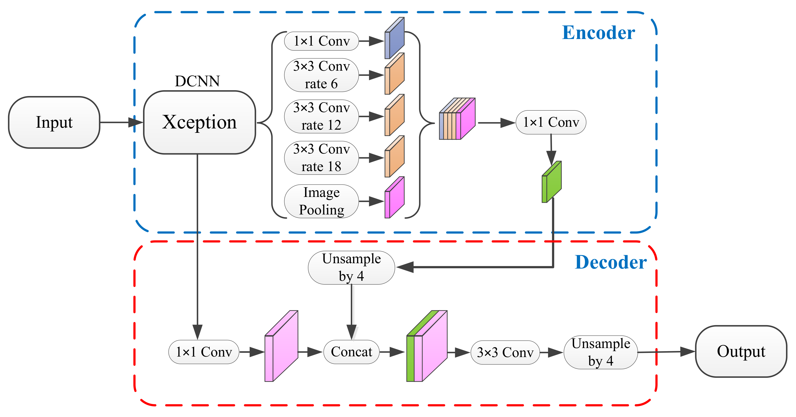
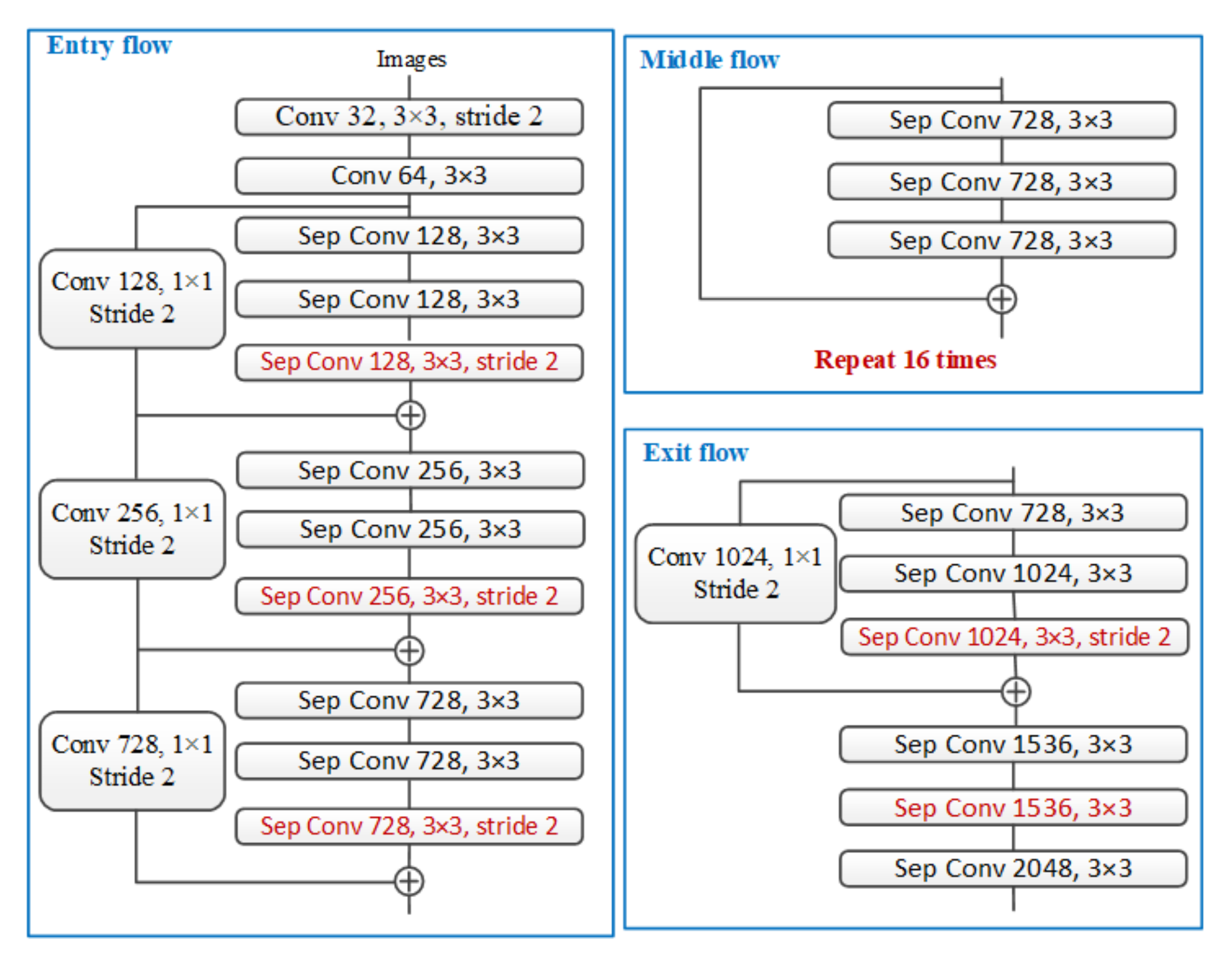
2. DeepLabv3+ Algorithm

DeepLabv3+ is one of the best semantic segmentation algorithms currently. On the basis of DeepLabv3, this algorithm forms a coding-decoding structure by adding a concise and effective decoder. The overall network structure of DeepLabv3+ is shown in Figure 2.

As can be seen from Figure 2, the encoding part is mainly composed of the backbone network and the atrous spatial pyramid pooling (ASPP) module. The decoding part upsamples the output feature map obtained from the encoding part and concatenates it with the low-dimensional feature map, then bilinear interpolation is used to restore the size of the input image to get the final segmentation result.

In the encoding phase, DeepLabv3+ uses the optimized and improved Xception network as the backbone network to extract features, and the optimized and improved Xception network structure is shown in Figure 3.

As can be seen from Figure 3, the optimization of the network structure is mainly reflected in the following aspects: (a) the middle flow in the original Xception structure is repeated more times, and the network structure is deepened; (b) the depth-wise separable convolution is used to replace the max pooling in the original network, so that the network can extract the feature maps at any resolution by using atrous separable convolution; (c) referring to the design of MobileNet, batch normalization and ReLU (Rectified Linear Unit) activation are added after each 3 × 3 depth-wise convolution.

The atrous spatial pyramid pooling module adopts a parallel structure, and this module uses atrous convolution with different atrous rates to obtain multi-scale information. As can be seen from the DeepLabv3+ network structure, the ASPP module contains a 1 × 1 convolution, three 3 × 3 atrous convolution with atrous rates of 6, 12, 18, and a global average pooling branch, and there is a batch normalization layer for data normalization after each operation. The feature maps obtained by each branch are concatenated, finally a 1 × 1 convolution is used to compress and integrate features.

The structure of the decoding part is relatively simple. The final output of the encoding part of the network is a high-dimensional feature map with 256 channels. After the feature map is sent to the decoder, it is first up-sampled by bilinear interpolation, then concatenated with low-level features with the same resolution in the backbone network. In order to prevent the number of channels with more low-level features from having a great influence on the semantic information in the high-level features, the network uses 1 × 1 convolution of the low-level features to reduce channels before the feature concatenated. The concatenated features go through a 3 × 3 convolution to refine the features, and then use bilinear interpolation 4 times up-sampling to restore to the size of the original image to obtain the final detection result.

The encoder-decoder structure adopted by DeepLabv3+ is relatively novel. The encoder is mainly used to encode rich context information, while the concise and efficient decoder is used to restore the boundary of the detected object. In addition, the network uses atrous convolution to realize the feature extraction of the encoder at any resolution, so that the network can better balance detection speed and detection accuracy.

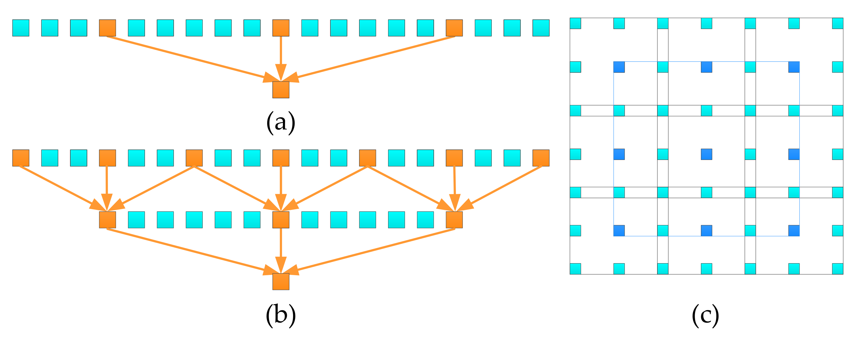
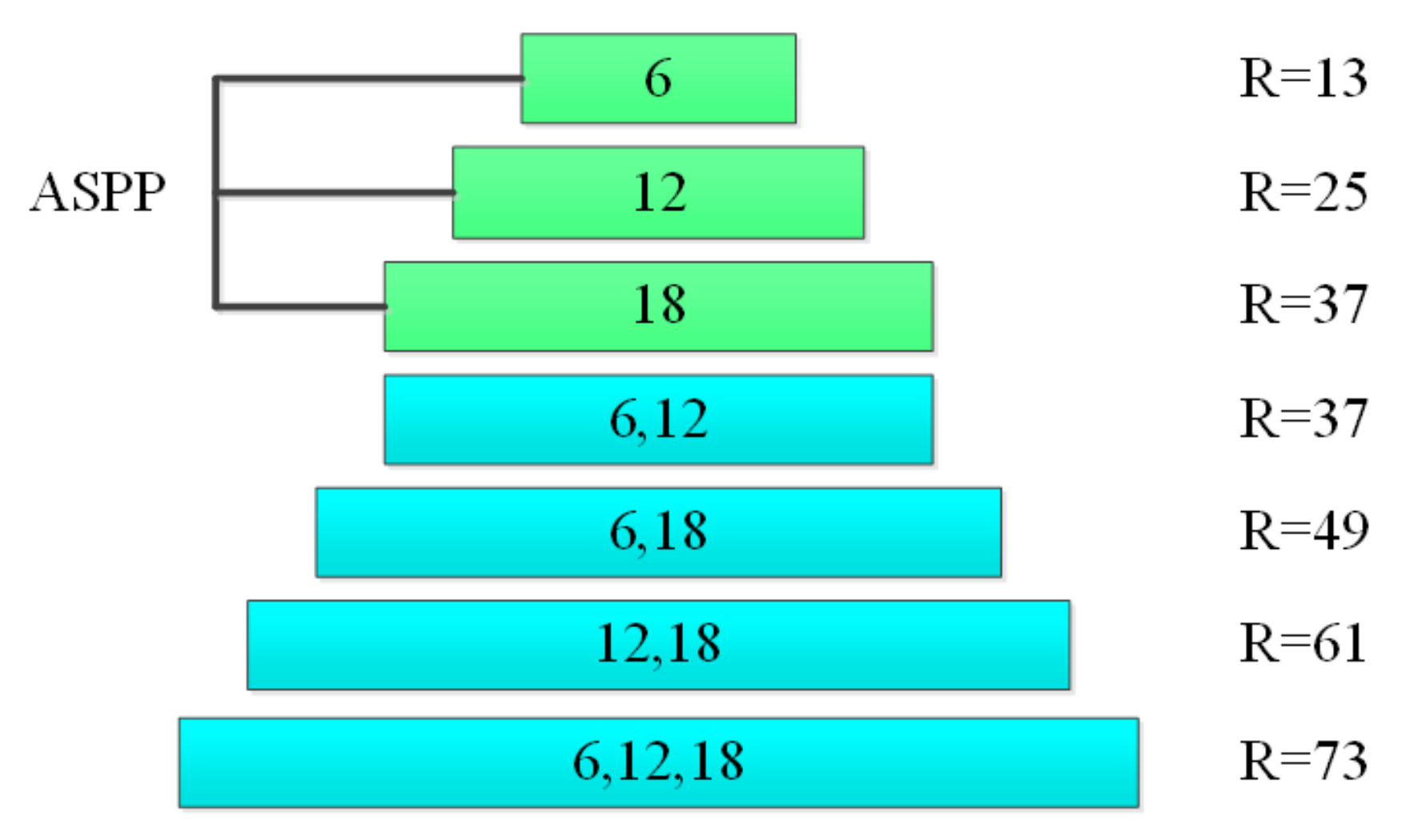
3. Dense-DeepLabv3+ Semantic Segmentation Algorithm

In view of the small and irregular distribution of bridge cracks, in order to enable the network to better extract the crack characteristics, based on the original DeepLabv3+ network structure, the atrous spatial pyramid pooling module is changed from the original method of independent branches. The dense connection method can achieve denser pixel sampling and improve the feature extraction ability of the algorithm. The improved Dense-DeepLabv3+ network structure is shown in Figure 4.

In Figure 4, referring to the network structure of DenseNet [42], the ASPP module of the DeepLabv3+ network is improved through dense connection, as shown in the yellow dashed box in Figure 4. Compared with Figure 2, the series structure is added on the basis of the original three atrous convolutions in parallel. The output of the atrous convolution with a smaller atrous rate and the output of the backbone network are concatenated, and then they are sent to the atrous convolution with a larger atrous rate together to achieve a better feature extraction effect.

The densely connected ASPP module can use more pixels in the calculation. The pixel sampling of atrous convolution is sparser than that of ordinary convolution. Taking one-dimensional atrous convolution as an example, the receptive field of one-dimensional atrous convolution is 13 when the atrous rate is 6, as shown in Figure 5a.

It can be seen from Figure 5a that when the convolution operation is performed on the atrous convolution, only 3 pixels are used for calculation each time. This situation will be worse in the two-dimensional convolution operation.

After the ASPP module is densely connected, the atrous rate increases layer by layer, and the layer with the larger atrous rate uses the output of the layer with the smaller atrous rate as input, which makes the pixel sampling denser and improves the utilization of pixels. As shown in Figure 5b, the atrous convolution with an atrous rate of 3 is performed before the atrous convolution with an atrous rate of 6, so that 7 pixels in the final convolution result are involved in the operation, and the sampling density is higher than that directly performed by the atrous convolution with the atrous rate of 6. When this situation extends to two dimensions, only 9 pixels are involved in the single-layer atrous convolution, while 49 pixels are involved in the cascaded atrous convolution, as shown in Figure 5c. As a result, the output of the lower atrous rate layer is connected to the larger atrous rate layer as input by the way of dense connection, and the ability of network feature extraction is enhanced.

The densely connected ASPP module can not only obtain denser pixel sampling, but also provide a larger receptive field. Atrous convolution can obtain larger receptive field without changing the resolution of the feature map. For atrous convolution with atrous rate $r$ and convolution kernel size $k$, the size of receptive field $R$ is:

$$R=(r-1)\times (k-1)+k$$

(1)

A larger receptive field can be obtained by stacking two atrous convolutions, and the size of the stacked receptive field can be obtained by the following formula:

$$R=R_1+R_2-1$$

(2)

where $R_1$ and $R_2$ are the receptive field sizes of the two atrous convolutions respectively. The receptive field size of the dense connection method obtained by stacking atrous convolution is shown in Figure 6.

The original ASPP module works in parallel, and each branch does not share any information, while the improved module realizes information sharing through layer-jumping connection. The atrous convolution of different atrous rates depend on each other, which increases the range of receptive field. Using $R_k^r$ to denote the receptive field provided by the atrous convolution with atrous rate $r$ and convolution kernel size $k$, and it is known from Equation (1) that the maximum receptive field $R_{\max }$ of the original ASPP module is:

$$R_{\max }=\max (R_3^6,R_3^{12},R_3^{18})=R_3^{18}=37$$

(3)

It can be seen from Equation (2) that the maximum receptive field of the improved ASPP module is:

$$R_{\max }=R_3^6+R_3^{12}+R_3^{18}-2=73$$

(4)

Although the densely connected ASPP module can obtain denser pixel sampling and a larger receptive field, it also increases the number of network parameters, which will affect the running speed of the network. In order to solve this problem, 1 × 1 convolution is used before each atrous convolution after dense connection to reduce the number of channels of the feature map, so as to reduce the number of parameters of the network and improve the expression ability of the network.

Let $c_0$ represent the number of channels of the input feature map of the ASPP module, $c_l$ represents the number of channels of the input feature map of the 1 × 1 convolution before the l-th atrous convolution, and $n$ represents the number of channels of the output feature map of each atrous convolution, the formula is as follows:

$$c_l=c_0+n\times (l-1)$$

(5)

The optimized Xception network is used as the backbone network, the feature map with 2048 output channels of the Xception network is used as the input of the ASPP module, and the number of channels $n$ of the output feature map of each atrous convolution of the ASPP module is 256, then the parameter number $S$ of the improved ASPP module can be calculated by the following formula:

$$S={\displaystyle {\sum }_{l=1}^L\left(c_l\times 1^2\times \frac{c_0}{2}+\frac{c_0}{2}\times k^2\times n\right)}=14155776$$

(6)

where $L$ is the number of atrous convolution, $k$ is the kernel size of atrous convolution.

In the original DeepLabv3+ network, the number of parameters of the ASPP module is as follows:

$$S=c_0\times k^2\times n\times L=14155776$$

(7)

From the results of the above two equations, it can be seen that the densely connected ASPP module in this paper successfully keeps the number of parameters the same as the original algorithm while obtaining denser pixel sampling and larger receptive field.

4. Crack Segmentation Results and Analysis

4.1. Evaluation Metrics

Evaluation metrics are used to evaluate the detection effect of the semantic segmentation model. Common evaluation metrics include pixel accuracy (PA), mean pixel accuracy (MPA), mean intersection over union (MIoU), etc. Assuming there are $m$ categories, and the background part is counted as an additional category, $p_{ii}$ represents the number of pixels that are correctly classified, $p_{ij}$ presents the number of pixels that belong to the i-th category but are classified into the j-th category. The definition of each evaluation metric is as follows.

Pixel accuracy (PA): calculates the ratio of the number of correctly classified pixels to the number of all pixels.

$$PA=\frac{{\displaystyle \sum _{i=0}^m{p}_{ii}}}{{\displaystyle \sum _{i=0}^m{\displaystyle \sum _{j=0}^m{p}_{ij}}}}$$

(8)

Mean pixel accuracy (MPA): the proportion of correctly classified pixels is calculated by class, and finally averaged by the total number of classes.

$$MPA=\frac{1}{m+1}{\displaystyle \sum _{i=0}^m\frac{p_{ii}}{{\displaystyle \sum _{j=0}^m{p}_{ij}}}}$$

(9)

Mean intersection over union (MIoU): this is a standard evaluation metric for segmentation problems, which calculates the overlap ratio of the intersection and union of two sets.

$$MI\mathrm{oU}=\frac{1}{m+1}{\displaystyle \sum _{i=0}^m\frac{p_{ii}}{{\displaystyle \sum _{j=0}^m{p}_{ij}+{\displaystyle \sum _{j=0}^m{p}_{ji}-p_{ii}}}}}$$

(10)

Among the above metrics, MIoU is an important metric to measure segmentation accuracy, and is the most commonly used in semantic segmentation algorithms. Therefore, the MIoU is selected as the final evaluation metric in this paper.

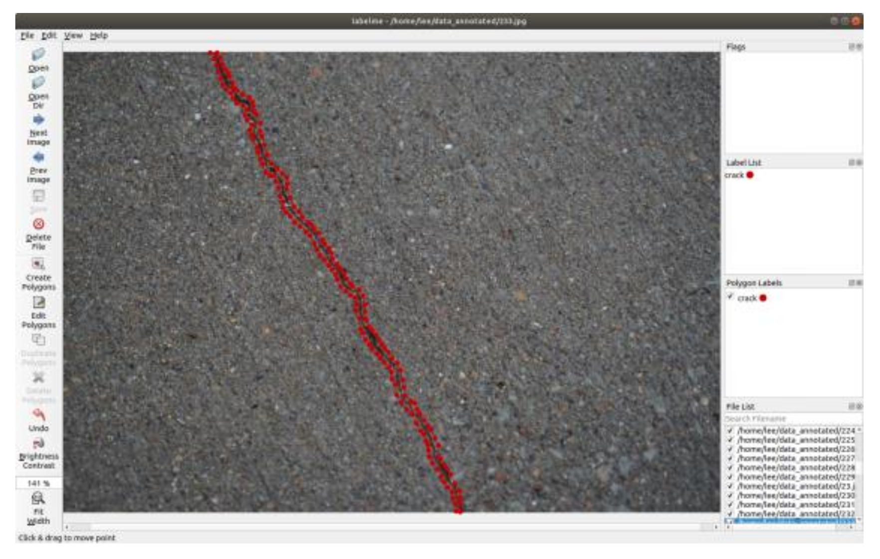
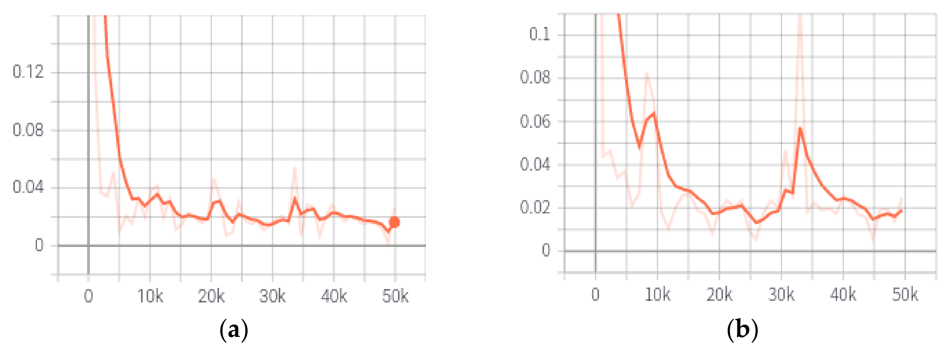
4.2. Experimental Conditions and Model Training

The experimental environment of this paper is configured with Ubuntu18.04 operating system, Intel Core i7-7700 CPU processor, NVIDIA GeForce GTX 1080Ti graphics card and TensorFlow deep learning framework. The original data of the experiment are obtained by collecting the real bridge crack images with digital equipment and from the Internet in various environments, such as humid environment, shadow, different surfaces and so on. The collected image is expanded by clipping, flipping, rotation, scaling and other operations. Finally, 5000 crack images with 600 × 400 pixels are obtained as the initial data set of this experiment.

The LabelMe tool is used to label the image, and the corresponding label map of the image is obtained after subsequent conversion processing. The crack data annotation is shown in Figure 7. Randomly divide the images in the data set, including 80% as the training set, 10% as the validation set, 10% as the test set, and package the divided data into a TFRecord (TensorFlow Record) format suitable for network input.

The training parameters of the original DeepLabv3+ and Dense-DeepLabv3+ network are shown in

Table 1. Network parameters setting table.

Training Parameters	Original DeepLabv3+	Dense-DeepLabv3+
Atrous rates	6, 12, 18	6, 12, 18
Base learning rate	0.001	0.001
Output stride	16	16
Train crop size	513, 513	513, 513
Train batch size	4	4
Training number of steps	50,000	50,000

.

In order to accelerate the convergence speed of network training, the training process loads the pre-trained improved Xception network weights. The initial learning rate of the experiment is 0.001, and the Adam optimization trainer is used.

The network was trained with different iteration times. When the number of training iterations is 50,000, the network effect is better. Using the TensorBoard tool that comes with TensorFlow to display the loss value changes during the training. The final training loss curve and validation loss curve of the Dense-DeepLabv3+ network is shown in Figure 8.

In Figure 8, the x-axis is the number of training iterations, and the y-axis is the network loss value. It can be seen from Figure 8 that due to the loading of the pre-trained model, the training loss value and validation loss curve can be reduced to a lower value in a few iterations. It also can be seen that the loss value maintains a downward trend until it finally converges. The training loss value drops to a relatively small value when the number of iterations is greater than 10,000. The overall effect of training is ideal.

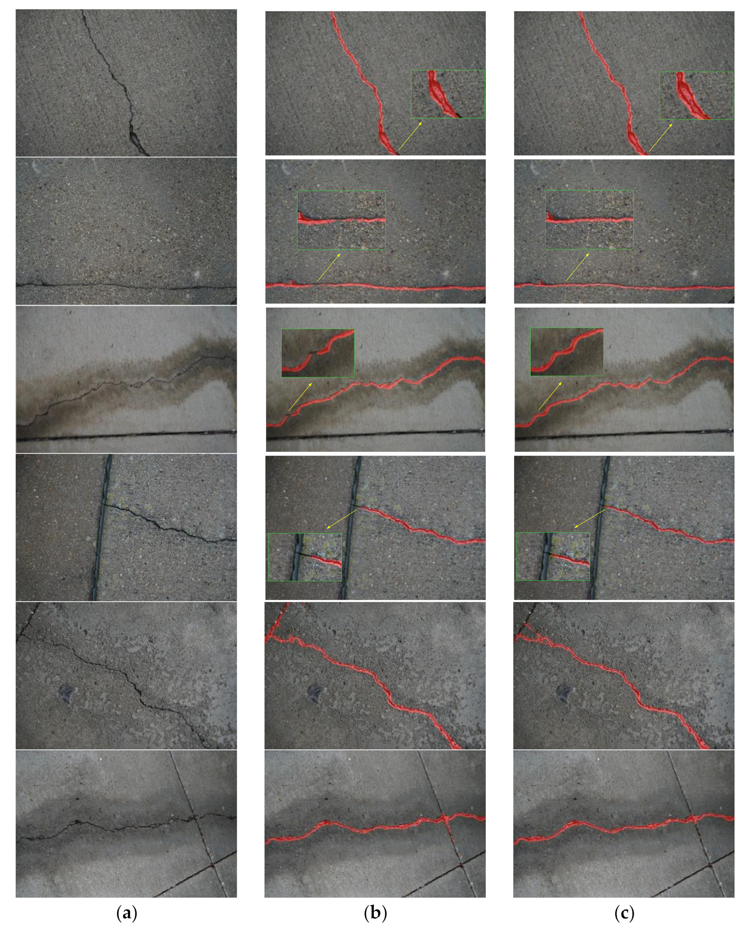
4.3. Crack Segmentation Experimental Results

In order to verify the effectiveness of the algorithm, the segmentation effect of the bridge crack image was tested. The original DeepLabv3+ network and the improved DeepLabv3+ network was tested on the same data set, and MIoU was selected as the final evaluation index. The test results are shown in

Table 2. Comparison of original DeepLabv3+ and Dense-DeepLabv3+ results.

	Class_0 [%]	Class_1 [%]	Overall [%]
original Deeplabv3+	99.12	58.74	78.93
Dense-DeepLabv3+	99.30	65.44	82.37

. Where Class_0 represents the MIoU value of the background part except the crack, Class_1 represents the MIoU value of the crack, and Overall represents the overall MIoU value.

As can be seen from the Table 2, compared with using the original DeepLabv3+ algorithm to segment the bridge crack image, the segmentation effect of Dense-DeepLabv3+ is better. The overall MIoU value is increased by 3.44%, and the segmentation effect of the bridge crack region is improved more obviously, the MIoU value is increased by 6.70%. The experiment results show that the improved DeepLabv3+ network is effective for bridge crack image segmentation. Due to space limitations, only some representative segmentation results are given, as shown in Figure 9. In order to see the crack segmentation effect clearly, the segmentation result image is overlaid on the original image. Because the image size of the crack segmentation results in the paper are small, some magnified images with highlighted boxes are provided, so that the details of the segmentation results can be displayed more clearly.

In Figure 9, the first column is the original images, the second column is the original DeepLabv3+ segmentation results, and the third column is the Dense-DeepLabv3+ segmentation results. It can be seen from the first row that both the original algorithm and the improved algorithm can detect bridge cracks, but the segmentation result of the improved algorithm is more detailed. From the second and third rows, the cracks in the image are continuous, and the detection results of the original DeepLabv3+ algorithm appear discontinuous, while the crack detection results of the Dense-DeepLabv3+ algorithm are continuous and complete. It can be seen from the fourth row that the segmentation result of the original DeepLabv3+ algorithm missed a small section of cracks, while the segmentation result of the improved algorithm is relatively complete. From the fifth and sixth rows we can see that the original DeepLabv3+ algorithm mistakenly detects the normal construction gap as a crack, and the Dense-DeepLabv3+ algorithm avoids this problem. When there are water stains in the crack image, it can also detect cracks with good robustness. The segmentation results show that the Dense-DeepLabv3+ algorithm has a better segmentation effect on the bridge crack images, and the segmentation results are more accurate than the original DeepLabv3+ algorithm.

In the process of crack detection, there are also cases of inaccurate detection, such as the case shown in Figure 10.

Due to the blurring at the edge of the image, and few data samples being available for such cases, the cracks at the edge of the image are not well detected in Figure 10. To improve the detection accuracy, some image preprocessing methods such as deblurring can be added, and the number of training samples of this type can be increased to improve the detection accuracy. In our future work, the crack detection algorithm will be studied with low-quality images.

5. Conclusions

Aiming at the task of crack image segmentation in a bridge crack detection system, a bridge crack image segmentation algorithm based on Dense-DeepLabv3+ network was proposed in this paper. In the part of the network structure, the ASPP module in the original network was changed from the parallel structure of each branch to a densely connected form, which realizes denser and multi-scale information encoding, obtains denser pixel sampling and larger receptive field, and reasonably controls the number of parameters of the network. Segmentation experiments were carried out on the bridge crack data set using the proposed algorithm, and the experimental results showed that the crack detection effect of the improved algorithm were better than the original algorithm. The overall MIoU value reached 82.37%, which was 3.44% higher than the original DeepLabv3+ algorithm, and had higher segmentation accuracy.

References

1. Sabatino, S.; Frangopol, D.M.; Dong, Y. Sustainability-informed maintenance optimization of highway bridges considering multi-attribute utility and risk attitude. Eng. Struct. 2015, 102, 310–321. [Google Scholar] [CrossRef]
2. Cheng, H.D.; Shi, X.J.; Glazier, C. Real-time image thresholding based on sample space reduction and interpolation approach. J. Comput. Civ. Eng. 2003, 17, 264–272. [Google Scholar] [CrossRef]
3. Rao, S.R.; Mobahi, H.; Yang, A.Y.; Sastry, S.S.; Yi, M. Natural image segmentation with adaptive texture and boundary encoding. In Proceedings of the Asian Conference on Computer Vision, Xi’an, China, 23–27 September 2009; Springer: Berlin/Heidelberg, Germany, 2009; pp. 135–146. [Google Scholar]
4. Xu, J.X.; Zhang, X.N. Crack detection of reinforced concrete bridge using video image. J. Cent. South Univ. 2013, 20, 2605–2613. [Google Scholar] [CrossRef]
5. Mokhtari, S.; Wu, L.L.; Yun, H.B. Comparison of Supervised Classification Techniques for Vision-Based Pavement Crack Detection. Transp. Res. Rec. 2016, 2595, 119–127. [Google Scholar] [CrossRef]
6. Hoang, N.D.; Nguyen, Q.L. A novel method for asphalt pavement crack classification based on image processing and machine learning. Eng. Comput. 2019, 35, 487–498. [Google Scholar] [CrossRef]
7. Liu, L.; Ouyang, W.L.; Wang, X.G.; Fieguth, P.; Chen, J.; Liu, X.W.; Pietikinen, M. Deep Learning for Generic Object Detection: A Survey. Int. J. Comput. Vis. 2020, 128, 261–318. [Google Scholar] [CrossRef] [Green Version]
8. Girshick, R.; Donahue, J.; Darrell, T.; Malik, J. Rich feature hierarchies for accurate object detection and semantic segmentation. In Proceedings of the IEEE Conference on Computer Vision and Pattern Recognition, Columbus, OH, USA, 23–28 June 2014; pp. 580–587. [Google Scholar]
9. Girshick, R. Fast R-CNN. In Proceedings of the IEEE International Conference on Computer Vision, Santiago, Chile, 11–18 December 2015; pp. 1440–1448. [Google Scholar]
10. Ren, S.Q.; He, K.; Girshick, R.; Sun, J. Faster R-CNN: Towards Real-Time Object Detection with Region Proposal Networks. IEEE Trans. Pattern Anal. Mach. Intell. 2017, 39, 1137–1149. [Google Scholar] [CrossRef] [Green Version]
11. Redmon, J.; Divvala, S.; Girshick, R.; Farhadi, A. You Only Look Once: Unified, Real-Time Object Detection. In Proceedings of the IEEE Conference on Computer Vision and Pattern Recognition, Seattle, WA, USA, 27–30 June 2016; pp. 779–788. [Google Scholar]
12. Redmon, J.; Farhadi, A. YOLO9000: Better, Faster, Stronger. In Proceedings of the IEEE/CVF Conference on Computer Vision and Pattern Recognition, Honolulu, HI, USA, 21–26 July 2017; pp. 6517–6525. [Google Scholar]
13. Redmon, J.; Farhadi, A. YOLOv3: An Incremental Improvement. arXiv 2018, arXiv:1804.02767. [Google Scholar]
14. Bochkovskiy, A.; Wang, C.Y.; Liao, H.Y.M. YOLOv4: Optimal Speed and Accuracy of Object Detection. arXiv 2020, arXiv:2004.10934. [Google Scholar]
15. Liu, W.; Anguelov, D.; Erhan, D.; Szegedy, C.; Reed, S.; Fu, C.Y.; Berg, A.C. SSD: Single Shot MultiBox Detector. In Proceedings of the European Conference on Computer Vision, Amsterdam, The Netherlands, 8–16 October 2016; pp. 21–37. [Google Scholar]
16. Lin, T.Y.; Goyal, P.; Girshick, R.; He, K.M.; Dollar, P. Focal Loss for Dense Object Detection. In Proceedings of the IEEE International Conference on Computer Vision, Venice, Italy, 22–29 October 2017; pp. 318–327. [Google Scholar]
17. Law, H.; Deng, J. CornerNet: Detecting Objects as Paired Keypoints. In Proceedings of the European Conference on Computer Vision, Munich, Germany, 8–14 September 2018; pp. 642–656. [Google Scholar]
18. Zhou, X.Y.; Zhuo, J.C.; Krahenbuhl, P. Bottom-up Object Detection by Grouping Extreme and Center Points. In Proceedings of the IEEE/CVF Conference on Computer Vision and Pattern Recognition, Long Beach, CA, USA, 16–20 June 2019; pp. 850–859. [Google Scholar]
19. Zhou, X.; Wang, D.; Krähenbühl, P. Objects as points. arXiv 2019, arXiv:1904.07850. [Google Scholar]
20. Long, J.; Shelhamer, E.; Darrell, T. Fully Convolutional Networks for Semantic Segmentation. In Proceedings of the IEEE Conference on Computer Vision and Pattern Recognition, Boston, MA, USA, 7–12 June 2015; pp. 3431–3440. [Google Scholar]
21. Badrinarayanan, V.; Kendall, A.; Cipolla, R. SegNet: A Deep Convolutional Encoder-Decoder Architecture for Image Segmentation. IEEE Trans. Pattern Anal. Mach. Intell. 2017, 39, 2481–2495. [Google Scholar] [CrossRef]
22. Ronneberger, O.; Fischer, P.; Brox, T. U-Net: Convolutional Networks for Biomedical Image Segmentation. In Proceedings of the International Conference on Medical Image Computing and Computer-Assisted Intervention, Munich, Germany, 5–9 October 2015; pp. 234–241. [Google Scholar]
23. Chen, L.C.; Papandreou, G.; Kokkinos, I.; Murphy, K.; Yuille, A. Semantic Image Segmentation with Deep Convolutional Nets and Fully Connected CRFs. In Proceedings of the 3rd International Conference on Learning Representations, San Diego, CA, USA, 7–9 May 2015; pp. 357–361. [Google Scholar]
24. Chen, L.C.; Papandreou, G.; Kokkinos, I.; Murphy, K.; Yuille, A. DeepLab: Semantic Image Segmentation with Deep Convolutional Nets, Atrous Convolution, and Fully Connected CRFs. arXiv 2016, arXiv:1606.00915v2. [Google Scholar] [CrossRef]
25. Chen, L.C.; Papandreou, G.; Schroff, F.; Adam, H. Rethinking atrous convolution for semantic image segmentation. arXiv 2017, arXiv:1706.05587. [Google Scholar]
26. Chen, L.C.; Zhu, Y.K.; Papandreou, G.; Schroff, F.; Adam, H. Encoder-Decoder with Atrous Separable Convolution for Semantic Image Segmentation. In Proceedings of the European Conference on Computer Vision, Munich, Germany, 8–14 September 2018; pp. 833–851. [Google Scholar]
27. Zhao, H.S.; Shi, J.P.; Qi, X.J.; Wang, X.G.; Jia, J.Y. Pyramid Scene Parsing Network. In Proceedings of the IEEE/CVF Conference on Computer Vision and Pattern Recognition, Honolulu, HI, USA, 21–26 July 2017; pp. 6230–6239. [Google Scholar]
28. Zhang, L.; Yang, F.; Zhang, Y.D.; Zhu, Y.J. Road crack detection using deep convolutional neural network. In Proceedings of the 2016 IEEE International Conference on Image Processing, Phoenix, AZ, USA, 25–28 September 2016; pp. 3708–3712. [Google Scholar]
29. Cha, Y.J.; Choi, W.; Büyüköztürk, O. Deep Learning-Based Crack Damage Detection Using Convolutional Neural Networks. Comput. Aided Civ. Infrastruct. Eng. 2017, 32, 361–378. [Google Scholar] [CrossRef]
30. An, Y.K.; Jang, K.; Kim, B.; Cho, S. Deep learning-based concrete crack detection using hybrid images. In Proceedings of the Conference on Sensors and Smart Structures Technologies for Civil, Mechanical, and Aerospace Systems, Denver, CA, USA, 5–8 March 2018; p. 10598. [Google Scholar]
31. Zhang, A.; Wang, K.C.; Fei, Y.; Liu, Y.; Tao, S.; Chen, C.; Li, J.Q.; Li, B. Deep Learning-Based Fully Automated Pavement Crack Detection on 3D Asphalt Surfaces with an Improved CrackNet. J. Comput. Civ. Eng. 2018, 32, 04018041. [Google Scholar] [CrossRef] [Green Version]
32. Nie, M.; Wang, C. Pavement Crack Detection based on yolo v3. In Proceedings of the 2nd International Conference on Safety Produce Informatization, Chongqing, China, 28–30 November 2019; pp. 327–330. [Google Scholar]
33. Lee, D.; Kim, J.; Lee, D. Robust Concrete Crack Detection Using Deep Learning-Based Semantic Segmentation. Int. J. Aeronaut. Space Sci. 2019, 20, 287–299. [Google Scholar] [CrossRef]
34. Lyu, P.H.; Wang, J.; Wei, R.Y. Pavement Crack Image Detection based on Deep Learning. In Proceedings of the International Conference on Deep Learning Technologies, Xiamen, China, 5–7 July 2019; pp. 6–10. [Google Scholar]
35. Zou, Y.; Cao, W.; Luo, M.; Zhang, P.; Wang, W.; Huang, W. Deep Learning-based Pavement Cracks Detection via Wireless Visible Light Camera-based Network. In Proceedings of the IEEE International Conference on Computing, Communications and IoT Applications, Shenzhen, China, 26–28 October 2019; pp. 47–52. [Google Scholar]
36. Huyan, J.; Li, W.; Tighe, S.; Xu, Z.C.; Zhai, J.Z. CrackU-net: A novel deep convolutional neural network for pixelwise pavement crack detection. Struct. Control Health Monit. 2020, 27, e2551. [Google Scholar] [CrossRef]
37. Park, S.E.; Eem, S.H.; Jeon, H. Concrete crack detection and quantification using deep learning and structured light. Constr. Build. Mater. 2020, 252, 119096. [Google Scholar] [CrossRef]
38. Yang, Q.; Shi, W.; Chen, J.; Lin, W. Deep convolution neural network-based transfer learning method for civil infrastructure crack detection. Autom. Constr. 2020, 116, 103199. [Google Scholar] [CrossRef]
39. Kalfarisi, R.; Wu, Z.Y.; Soh, K. Crack Detection and Segmentation Using Deep Learning with 3D Reality Mesh Model for Quantitative Assessment and Integrated Visualization. J. Comput. Civ. Eng. 2020, 34, 04020010. [Google Scholar] [CrossRef]
40. Billah, U.H.; La, H.M.; Tavakkoli, A. Deep Learning-Based Feature Silencing for Accurate Concrete Crack Detection. Sensors 2020, 20, 4403. [Google Scholar] [CrossRef]
41. Fang, F.; Li, L.; Gu, Y.; Zhu, H.; Lim, J.H. A Novel Hybrid Approach for Crack Detection. Pattern Recogn. 2020, 107, 107474. [Google Scholar] [CrossRef]
42. Huang, G.; Liu, Z.; van der Maaten, L.; Weinberger, K.Q. Densely Connected Convolutional Networks. In Proceedings of the IEEE Conference on Computer Vision and Pattern Recognition, Honolulu, HI, USA, 21–26 July 2017; pp. 2261–2269. [Google Scholar]
Figure 1. Manual bridge crack detection.
Jmse 09 00671 g001
Figure 2. DeepLabv3+ network structure.
Jmse 09 00671 g002
Figure 3. Improved Xception network structure.
Jmse 09 00671 g003
Figure 4. Dense-DeepLabv3+ network structure.
Jmse 09 00671 g004
Figure 5. Schematic diagram of atrous convolution. (a) one dimensional atrous convolution operation (b) improved one-dimensional atrous convolution operation (c) improved two-dimensional atrous convolution operation.
Jmse 09 00671 g005
Figure 6. Receptive field of dense connection.
Jmse 09 00671 g006
Figure 7. The crack data annotation.
Jmse 09 00671 g007
Figure 8. The training and validation loss curve of the Dense-DeepLabv3+. (a) training loss curve (b) validation loss curve.
Jmse 09 00671 g008
Figure 9. Comparison of original DeepLabv3+ and Dense-DeepLabv3+ crack segmentation results. (a) original image (b) DeepLabv3+ (c) Dense-DeepLabv3+.
Jmse 09 00671 g009
Figure 10. Comparison of original DeepLabv3+ and Dense-DeepLabv3+ crack segmentation results. (a) original image (b) Dense-DeepLabv3+.
Jmse 09 00671 g010