A New Marine Disaster Assessment Model Combining Bayesian Network with Information Diffusion

Abstract

There are two challenges in the comprehensive marine hazard assessment. The influencing mechanism of marine disaster is uncertain and disaster data are sparse. Aiming at the uncertain knowledge and small sample in assessment modeling, we combine the information diffusion algorithm and Bayesian network to propose a novel assessment model. The information diffusion algorithm is adopted to expand associated samples between disaster losses and environmental conditions. Then the expanded data sets are used to build the BN-based assessment model through structural learning, parameter learning and probabilistic reasoning. The proposed model is applied to the hazard assessment of marine disasters in Shanghai. Experimental comparison results show that it is capable of dealing with uncertainty effectively and achieving more accuracy risk assessment under the small sample condition.

1. Introduction

The 21st century has been widely recognized as “A Century of Ocean”. Ocean, as the main space of marine development and security strategy, plays a significant role in safeguarding national security, alleviating resource shortages and expanding the development space for economy and society. It is well known that the marine environment involves numerous oceanic and meteorological factors, which are constantly changing and have complex mutual actions between each other. With climate change, marine disasters are occurring more frequently and disaster losses are heavier. Risk assessment is taken increasingly seriously. However, the risk mechanism of marine disasters is nonlinear and uncertain. Besides this, statistical information of disasters is usually scarce, causing an obstacle to risk assessment. It is difficult to evaluate disaster risk under uncertain knowledge and lacking information conditions. Therefore, developing new assessment models becomes an important subject to be studied urgently.

Marine environment is complicated and varied, producing varieties of marine disasters, such as marine geologic disaster, red tide, wave disaster, sea ice disaster and storm surge disaster. Many scholars have carried out risk assessment studies on different types of marine disasters: Qiao focused on the hazard assessment of geologic disaster sources in coastal areas [1]. He constructed the evaluation system by classifying features of different risk sources such as fault and earthquake, then adopted the analytic hierarchy process (AHP) to assess the marine geologic hazard quantitatively. Wen [2] analyzed characteristics of risk-causing factors and risk-on bodies to set up the assessment index system and developed a new red tide risk assessment model. Yuan [3] selected systematic assessment indicators of the sea ice disaster with consideration of natural and anthropogenic environment, and put forward the theoretical basis and concrete method of disaster assessment and zoning. Ericken [4] applied the fuzzy clustering and fuzzy reasoning algorithm to deal with the fuzziness of sea ice disaster information, achieving the reasoning of uncertain information and the regional division of sea ice risk. Zhao [5] summarized the research progress of storm surge disaster assessment and constructed a multi-level indicator system from the aspects of nature, society and economy, then applied the principal component analysis and geographic information system to the risk assessment of storm surge disaster.

Marine disasters, occurring in the form of cluster, concurrence and contingency, usually cause considerable disaster losses. However, it is difficult to express these forms through the risk assessment of a single type of marine disaster. Several studies have been devoted to the comprehensive risk assessment of multiple marine disasters: Ye [6] analyzed the temporal–spatial characteristics of oceanic and meteorological variables and established the general risk management system of comprehensive marine disaster. Zhang [7] elaborated marine environmental features in the South China Sea from the perspectives of marine geography, marine meteorology and marine hydrology, and adopted the fuzzy synthetic evaluation method to evaluate the marine hazard. Dubois [8] designed an integrated risk analysis frame of multiple marine disasters in coastal areas, including unit division, identification of disaster-causing factors and vulnerability analysis of disaster bearing body. In addition, the Earth System Science Partnership started the proposal of integrated risk governance to analyze internal relations between marine disasters and climate change at different spatial–temporal scales [9]. The Federal Emergency Administration of the USA developed a natural hazard loss estimation software to evaluate and predict the risk losses caused by multiple marine disasters, including storm surges, sea waves and typhoons. Comprehensive risk assessment of multiple marine disasters, emphasizing systematization and interdisciplinarity, can integrate and analyze different types of marine disasters to establish a more comprehensive assessment index system. With the index system set up, varieties of mathematical models are combined for quantitative assessment. In our research, we lay emphasis on analyzing the hazard of disaster-causing factors and focus on the comprehensive hazard evaluation of marine disasters.

From a physical standpoint, marine disasters are the presence of interactions of geographical, meteorological and hydrological factors. The influence is nonlinear, and the action mechanism is fuzzy between each two environmental variables, causing the randomness in temporal-spatial distribution, occurring frequency and hazard intensity of marine disasters. Therefore, marine disasters have significant uncertainties, which concretely manifest in self-uncertainty, information uncertainty and cognitive uncertainty [10]. In the above assessment of marine disasters, whether for a single marine disaster or multiple marine disasters, most studies use qualitative and semi-quantitative assessment methods, mainly including Delphi method, AHP, grey comprehensive evaluation method (GCE) and fuzzy comprehensive evaluation method (FCE). The subjectivity and experience are too strong in the expert investigation method. The analytical function is a linear model with strict mathematical assumptions, which is difficult to model with large-scale evaluation indicators and nonlinear relationships in marine environments. Besides this, GCE and FCE can only deal with one kind of uncertainty, such as randomness or fuzziness, but they are hard to achieve the uncertainty reasoning comprehensively. In conclusion, the existing assessment approaches hardly process uncertain information and are incapable of achieving assessment with complex influencing mechanism. Therefore, developing new risk assessment models propitious to the marine environment would be impressive.

Bayesian Network (BN), on the basis of probability theory and graph theory, shows great advantage in the expression of uncertain knowledge and the reasoning of complex relationships. The abilities of prior knowledge combination, multi-source information fusion and uncertainty reasoning make BN an effective model to solve uncertain problems in complex systems. In recent years, some studies have applied BN in assessment with nonlinear uncertain problems and made some achievements. Aguilera [11] adopted the clustering analysis to grade indicators and determine node states. Then the hierarchical BN is constructed for groundwater quality evaluation. Li [12] improved the BN with the genetic algorithm and applied it to the risk assessment of sea ice disasters. Boutkhamouin [13] used the BN to identify causal relationships between evaluation indicators and targets, and adopted the uncertainty reasoning mechanism for probabilistic assessment of floods. Liu [14] introduced the BN to the hazard evaluation and management of flood disaster, and proposed the weighted BN to deal with correlated variables. Application of BN in risk assessment has become an inevitable development trend. However, to the best of our knowledge, the use of BN in the marine hazard assessment is very limited.

It should be noted that, as an emerging artificial intelligence algorithm, a large number of objective data is essential for BN to mine the influence relationships among variables quantitatively. Unfortunately, marine disaster data are mainly collected by means of social statistical surveys. The time series of these data are not long enough, and the continuity is poor, especially in the lack of associated information between disaster losses and environmental conditions. The limited sample size cannot effectively support BN training and disaster assessment modeling. Huang [15,16] proposed a small sample expansion algorithm based on information matrix, that is the information diffusion algorithm, and successfully applied it to natural disaster assessment, which effectively improved the accuracy in assessment with small sample numbers. Zhang [17] improved the diffusion function of the information diffusion algorithm and proposed a more universal non-uniform information diffusion algorithm. It is an effective method of processing the incomplete information. In addition, the information diffusion model has also been effectively applied to the evaluation modeling of earthquake risk and water shortage risk [18,19]. Therefore, we will use the information diffusion algorithm to expand samples and complete the objective construction of BN, given the advantage of the model in dealing with the scarcity of disaster samples.

Aiming at the problem of high uncertainty and scarcity of disaster data in marine hazard assessment, this paper combines information diffusion and BN to construct a comprehensive hazard assessment model of marine disasters. The information diffusion algorithm is used to expand small samples in order to obtain sufficient disaster data for BN training. Then the BN-based assessment model is constructed through structural learning, parameter learning and probabilistic reasoning. For the model verification, we apply the model to the monthly hazard assessment of marine disasters in Shanghai. The remainder of the paper is organized as follows: Section 2 presents the theory of BN and information diffusion. Section 3 introduces the specific techniques of the assessment model. The obtained results and analysis are shown in Section 4. Section 5 draws conclusions and summarizes the main findings.

2. Fundamental Theory

2.1. Bayesian Network

Bayesian Network (BN), which relies on the graph theory and probability theory, is not only a graphical expression of causal relationships among variables, but also a probabilistic reasoning technique for random variables [20]. It is a quantitative causal relation graph and can be represented by a binary $\mathrm{B}=<G,\theta >$:

• $G=\left(V,E\right)$ represents a directed acyclic graph. $V$ is a set of nodes where each one represents a variable in the knowledge domain. $E$ is a set of arcs, and a directed arc represents the causal dependency between two variables.
• $\theta$ is the network parameter, that is, the conditional probability distribution of network node. $\theta$ expresses the degree of mutual influence between two nodes and presents quantitative characteristics in the knowledge domain.

Assume a set of variables $V=\left(v_1,\cdots ,v_n\right)$. The mathematical basis of BN is Bayes Theorem showed by Equation (1), which is also the core principle of Bayesian inference.

$$\mathrm{P}\left(v_i|v_j\right)=\frac{\mathrm{P}\left(v_i,v_j\right)}{\mathrm{P}\left(v_j\right)}=\frac{\mathrm{P}\left(v_i\right)·\mathrm{P}\left(v_j|v_i\right)}{\mathrm{P}\left(v_j\right)}$$

(1)

where: $\mathrm{P}\left(v_i\right)$ is the prior probability, $\mathrm{P}\left(v_j|v_i\right)$ is the conditional probability and $\mathrm{P}(v_i|v_j)$ is the posterior probability. Based on $\mathrm{P}\left(v_i\right)$, $\mathrm{P}\left(v_i|v_j\right)$ can be derived with Bayes Theorem under the relevant conditions $\mathrm{P}\left(v_j|v_i\right)$.

The joint probability distribution for Bayesian network can be derived from Equation (1) under the conditional independence assumption, namely, each child node is independent of non-parent nodes under conditions given.

$$\mathrm{P}\left(v_1,v_2,\cdots v_n\right)={\displaystyle \prod }_{i=1}^n\mathrm{P}\left(v_i|\mathrm{Pa}\left(v_i\right)\right)$$

(2)

where: $v_i$ is network node; $\mathrm{Pa}\left(v_i\right)$ is parent node of $v_i$. Bayesian inference is the calculation of probability distribution of a set of query variables according to updated evidence of input variables through Equation (2).

The modeling procedure of BN mainly includes structural learning, parameter learning and probabilistic reasoning [21,22]. This process is specifically described as: firstly, mining causal relationships from the existing data sets to construct the network topology; then, learning the conditional probability distribution of each node that matches the objective data; and finally, performing network probabilistic inference based on the structure and parameter. In general, there are three BN modeling ways, presented in

Table 1. Modeling ways of BN.

Modeling Way	Explanation
Subjective Manual Construction	The causal relationships among nodes are identified based on expert knowledge and experience, and the probability distributions are subjectively assigned to the nodes in the network. This modeling method is simple and clear but subjective.
Objective Automatic Construction	The network structure and node parameter are determined through the analysis of large amounts of data. This modeling way avoids subjective experience, but the hypotheses of statistical algorithms make the rationality of the network questionable and ignores the knowledge fusion ability of the BN.
Combination Construction	Expert knowledge and objective data are combined to build and optimize the network structure and conditional probability distribution. This modeling method is suitable for complex systems by optimizing the BN continuously on the basis of the fusion of subjective and objective information.

. The hazard assessment of comprehensive marine disasters is a complicated system engineering and we will adopt the modeling way of combining subjective and objective analysis.

2.2. Information Diffusion

To solve the problems of data shortage and sample sparsity in natural disaster assessment, Huang [15] proposed the information diffusion algorithm by introducing the information matrix, which has been systematically applied to the risk analysis of earthquake disaster. This algorithm simulates the molecular diffusion process so that each sparse data point can be diffused to the neighboring area points with a certain probability according to the information degree [23]. Thus, the single value sample can be turned into a set value sample and the incomplete sample is effectively augmented.

The principle of information diffusion is: $X=\left\{X_1,X_2,\cdots ,X_n\right\}$ which is defined as a knowledge sample used to estimate the universe $U$. The observation of $X_i$ is denoted as $l_i$. When $X$ is incomplete, there exists a function $\mu \left(x\right)$ which can fit the information distribution of the original population well. According to this principle, the estimation of the population probability density function is called diffusion estimation [15].

Suppose $\mu \left(x\right)$ is a Borel measurable function in the internal (−∞, +∞). $x=\frac{l-l_i}{d}$ ($l$ represents any possible observation). The diffusion probability estimation of the population probability density function is:

$$f\left(l\right)=\frac{1}{nd}{\displaystyle \sum }_{i=1}^n\mu \left(\frac{l-l_i}{d}\right)$$

(3)

where: $\mu$ is diffusion function. $d$ is called bandwidth ($d>0$).

For a system of “input–output”: $\mathsf{\Omega }$ is the parent population. $x$, $y$ are input and output components of the domain $X\times Y$ respectively. $d_x$, $d_y$ represent the diffusion coefficient bandwidth of the input and output components. The probability density function $f\left(x,y\right)$ of the parent population $\mathsf{\Omega }$ reflects the information distribution density of the point $\left(x,y\right)$ in the space. $f\left(x,y\right)$ is often unknowable in reality, so its diffusion estimation $\widehat{f}\left(x,y\right)$ is substituted for $f\left(x,y\right)$. The small samples are regarded as “information injection points” scattered in the “input–output” domain, and each sample is extended to a fuzzy set representation of several surrounding sample points through set-valued processing [16].

Diffusion function $\mu$ and bandwidth $d$ are the key parameters of information diffusion. Scholars have proposed different parameter setting methods and constructed different information diffusion models, including the normal information diffusion model, the optimal information diffusion model and elliptical non-uniform information diffusion model [24,25,26]. All have achieved good performance in the field of risk assessment. In our research, we adopt the non-normal diffusion model based on the string vibration equation proposed by Bai [27] to carry out the sample expansion of marine disaster data. This model uses the string vibration equation as the diffusion function to improve the normal limitation of the diffusion function. Compared with the traditional information diffusion model, Bai’s model can be reasonable and more effective in extracting and expanding date structure information from the incomplete small samples.

3. Assessment Model

With the combination of information diffusion and Bayesian network, we construct the comprehensive hazard assessment model for multiple marine disasters, in order to achieve the assessment modeling with uncertain knowledge and small samples. As shown in Figure 1, the technical process is divided into three modules: sample expansion module, network learning module and probabilistic reasoning module.

• Sample Expansion Module: Select the representative evaluation indicators for the comprehensive hazard of marine disasters and collect disaster data, then use the information diffusion algorithm to expand the finite samples. Discretize the evaluation indicators to determine the state space taken by each indicator and obtain sufficient discrete samples used for BN learning.
• Network Learning Module: Take the evaluation indicators as network nodes. Based on the expanded samples, use intelligent algorithms to mine the causal relationship among nodes from objective data and quantitatively express the relationships in the form of conditional probability distribution. Thus, complete the structural and parameter learning of BN.
• Probabilistic Reasoning Module: Input the priori information of marine environmental variables, and use the precise reasoning mechanism based on Bayes theorem to perform probabilistic reasoning. Obtain the posterior probability distribution of the evaluation object, then determine the comprehensive hazard level of marine disasters.

4. Model Construction

It is well-known that the risk includes the hazard of risk-causing factors, the vulnerability of risk-bearing body and the risk-prevention capacity. We focus on the hazard assessment in our research. The proposed assessment model is used to evaluate and predict the monthly comprehensive hazard of marine disasters in Shanghai, which borders the Yangtze River and the East China Sea. There are many kinds of marine disasters in Shanghai with a high occurrence frequency and activity intensity. The marine environment is complicated, and disaster hazard has tremendous uncertainty. Detailed evaluation and prediction of overall marine hazard are of great significance for ensuring personal security, economic and social development, and city operation.

4.1. Indicator Analysis

The marine disasters threatening the security of Shanghai mainly include storm surges, ocean waves, sea level rise and tsunamis. Given the disaster-causing mechanism of different types of marine disasters and relevant literatures [6,7], we select five representative environmental variables that have a remarkable effect on maritime activities for assessment modeling: wind speed, wave height, flow velocity, sea surface height and sea surface temperature. Studies have shown that wind speed can pose a serious threat to navigation safety. Wave height and sea surface height can bring harm to coastal constructions. Sea surface temperature may cause the malfunction of devices in ships. The mode of action of these variables is summarized in

Table 2. The mode of action of variables.

Variables	Hazard-on Objects	Hazard Consequences
Wind speed Wave height Flow velocity Sea surface height Sea surface Temperature	Port Infrastructure Ship People	Pollution or blockade of straits and waterway Damage to port facilities Subversion of ships Loss of life and personal injury

. We will then construct the hazard assessment indicators for marine disasters based on the above meteorological and oceanic variables.

(1)

Gale hazard indicator ($d_w$)

The hazard of gale is described in two aspects: average wind speed and extreme wind speed. Calculate the monthly average wind speed and the monthly maximum wind speed. The indicator is constructed based on Equation (4) coming from Ref. [7].

$$d_w=0.4\times U_{mean}+0.6\times U_{max}$$

(4)

where: $U_{mean}$ and $U_{max}$ respectively represent the monthly average wind speed and the monthly maximum wind speed.

(2)

Wave hazard indicator ($d_h$)

The hazard of sea wave is described in two aspects: sea wave intensity and frequency of occurrence. According to the classification of wave intensity (

Table 3. Intensity class of waves.

Sea wave Intensity	Significant Wave Height ($\mathit{S}\mathit{w}\mathit{h}/\mathbf{m}$)
I	$4.0\le Swh<6.0$
II	$2.5\le Swh<4.0$
III	$1.3\le Swh<2.5$
IV	$0\le Swh<1.3$

) presented in Ref. [28], the monthly average number of different level of wave height (I, II, III, IV) are calculated respectively.

The indicator is constructed according to Ref. [28].

$$d_h=0.6\times N_1+0.25\times N_2+0.1\times N_3+0.05\times N_4$$

(5)

where: $N_1, N_2, N_3, N_4$ represent the monthly average number of I, II, III, IV wave height respectively.

(3)

Flow velocity hazard indicator ($d_f$)

The hazard of flow velocity is described in two aspects: average flow velocity and extreme flow velocity. Calculate the monthly average flow velocity and the monthly maximum flow velocity. The indicator is constructed based on Equation (6).

$$d_f=0.4\times S_{mean}+0.6\times S_{max}$$

(6)

where: $S_{mean}$ and $S_{max}$ represent the monthly average flow velocity and the monthly maximum flow velocity respectively. The weight configuration comes from Ref. [7].

(4)

Sea level rise hazard indicator ($d_l$)

The hazard of sea level rise is described in two aspects: intensity and frequency of sea level rise. According to the classification of sea level rise intensity (

Table 4. Grade of sea level rise.

Grade	Sea Level Rise Rate (mm/month)
I	$0.2\le rate<0.3$
II	$0.1\le rate<0.2$
III	$0\le rate<0.1$

) in Ref. [28], the monthly average number of different grade of sea level rise (I, II, III) are calculated respectively.

The indicator is constructed according to Equation (7).

$$d_l=0.7\times H_1+0.2\times H_2+0.1\times H_3$$

(7)

where: $H_1, H_2,H_3$ represent the monthly average number of I, II, III sea level rise respectively. The weight configuration comes from Ref. [28].

(5)

Sea surface temperature hazard indicator ($d_t$)

The hazard of sea surface temperature is described in two aspects: average sea surface temperature and extreme sea surface temperature. Calculate the monthly average sea surface temperature and the monthly maximum sea surface temperature. The indicator is constructed based on Ref. [7].

$$d_t=0.4\times T_{mean}+0.6\times T_{max}$$

(8)

where: $T_{mean}$ and $T_{max}$ respectively represent the monthly average sea surface temperature and the monthly maximum sea surface temperature.

Considering the characteristics of the meteorological and oceanic environment in Shanghai, April to November is a peak period for various marine disasters. Therefore, we focus on the monthly assessment of comprehensive marine hazard in this period. Data sets required for the indicator construction come from observation in Sheng Shan Station (National Marine Data Center: http://mds.nmdis.org.cn/, accessed on 31 May 2021).

In addition to constructing evaluation indicators, we need to quantitatively express the evaluation object. The objective of our research is the comprehensive hazard of marine disasters, denoted as $A$. In almost all references, the severity of the hazard of marine disasters is usually quantified by the direct economic loss. These data come from the China Marine Disaster Bulletin (http://www.soa.gov.cn/zwgk/hygb/zghyzhgb/) (accessed on 20 February 2021) and Shanghai Statistical Yearbook. On account of limited data recording and data storage, the time series of these data are not long enough and discontinuous. We looked up the statistical yearbook from 2005 to 2019 and only obtained 80 complete samples.

Different indicators have different orders of magnitude. In order to eliminate the impact of dimension and to speed up the training of BN, all indicators need to be normalized according to Equation (9).

$$X=\frac{x-x_{min}}{x_{max}-x_{min}}$$

(9)

where: $X$ is the normalized value; $x$ is the original value; $x_{max}$, $x_{min}$ denote maximum and minimum of original data.

Table 5. Limited normalized samples.

Sample ID	${\mathit{d}}_{\mathit{w}}$	${\mathit{d}}_{\mathit{h}}$	${\mathit{d}}_{\mathit{f}}$	${\mathit{d}}_{\mathit{l}}$	${\mathit{d}}_{\mathit{t}}$	$\mathit{A}$
1	0.54	0.36	1	0.83	0.04	0.53
2	0.54	0.39	1	0.75	0.03	0.53
3	0.06	0.57	1	1	0.39	0.34
⋮	⋮	⋮	⋮	⋮	⋮	⋮
80	0.86	0.79	0	0.64	0.41	0.77

shows the normalized data, whose sample size is very small. The structural learning and parameter learning of BN rely on big data to explore causal relationships among variables. However, the sample size is too small to be directly used for either conventional statistical analysis methods or data mining techniques for BN modeling. Next, we will expand the samples.

4.2. Sample Expansion

The non-normal information diffusion algorithm based on the string vibration equation is adopted to expand the disaster samples. The detailed algorithm principle is elaborated in Ref. [27], and we will not repeat it here. The specific implementation steps of sample expansion are presented as follows:

Step 1: The first 50 samples in Table 3 are taken as modeling samples, and the last 30 samples are taken as testing samples. Each sample is denoted as $S=\left\{X_i^1,X_i^2,X_i^3,X_i^4,X_i^5,Y_i\right\} \left(i=1, 2,\cdots ,50\right)$. $X^1,X^2,X^3,X^4,X^5, Y$ respectively represents assessment indicators $d_w,d_h,d_f,d_l,d_t$ and assessment target $A$. The information injection points are set as follows:

$$\begin{array}{c}{U}^1=\left\{0, 0.1, 0.2, 0.3, 0.4, 0.5, 0.6, 0.7, 0.8, 0.9, 1\right\}=\left\{U_x^1, x=1,2,\cdots ,11\right\};\\ U^2=\left\{0, 0.1, 0.2, 0.3, 0.4, 0.5, 0.6, 0.7, 0.8, 0.9, 1\right\}=\left\{U_y^2, y=1,2,\cdots ,11\right\};\\ U^3=\left\{0, 0.1, 0.2, 0.3, 0.4, 0.5, 0.6, 0.7, 0.8, 0.9, 1\right\}=\left\{U_z^3, z=1,2,\cdots ,11\right\};\\ U^4=\left\{0, 0.1, 0.2, 0.3, 0.4, 0.5, 0.6, 0.7, 0.8, 0.9, 1\right\}=\left\{U_m^4, m=1,2,\cdots ,11\right\};\\ U^5=\left\{0, 0.1, 0.2, 0.3, 0.4, 0.5, 0.6, 0.7, 0.8, 0.9, 1\right\}=\left\{U_n^5, n=1,2,\cdots ,11\right\};\\ V=\left\{0, 0.1, 0.2, 0.3, 0.4, 0.5, 0.6, 0.7, 0.8, 0.9, 1\right\}=\left\{V_l, l=1,2,\cdots ,11\right\}\end{array}$$

Step 2: The bandwidth of the information diffusion algorithm are calculated using the modeling samples, as shown in

Table 6. Bandwidth of indicators.

	${\mathit{d}}_{\mathit{w}}$	${\mathit{d}}_{\mathit{h}}$	${\mathit{d}}_{\mathit{f}}$	${\mathit{d}}_{\mathit{l}}$	${\mathit{d}}_{\mathit{t}}$	$\mathit{A}$
Bandwidth	2.78439	1.14304	0.69897	0.10234	0.07154	0.07294

.

Step 3: It is calculated the amount of information $q_i$ diffused by each sample (the ordinal number is $i$) to the information injection point $\left(U_x^1,U_y^2,U_z^3,U_m^4,U_n^5,V_l\right)$:

$$q_i\left(U_x^1,U_y^2,U_z^3,U_m^4,U_n^5,V_l\right)=u({\displaystyle \sum }_{i=1}^5{X}_i,Y_i,{\displaystyle \sum }_{i=1}^5{h}_i)$$

where: $u$ represents the diffusion function; $h_i$ represents the bandwidth corresponding to different evaluation indicators.

Step 4: The information matrix $Q$ is formed by the superposition of information volume $q$:

$$Q={\displaystyle \sum }_{i=1}^n{q}_i=\begin{array}{c}\left(U_1^1,U_1^2,\cdots ,U_1^5\right)\\ \left(U_1^1,U_1^2,\cdots ,U_2^5\right)\\ \begin{array}{c}⋮\\ \left(U_{x_t}^1,U_y^2,\cdots ,U_{n_t}^5\right)\end{array}\end{array}\left(\begin{array}{ccccc}{Q}_{11}& & Q_{12}& \cdots & Q_{21}\\ Q_{21}& & Q_{22}& & Q_{21}\\ & ⋮& & \ddots & ⋮\\ Q_{t1}& & Q_{t2}& \cdots & Q_{tl}\end{array}\right)$$

Step 5: $Q$ can generate fuzzy relation matrix $R=\left\{r_{\left(U_x^1,U_y^2,U_z^3,U_m^4,U_n^5,V_l\right)}\right\}$. The conversion relationship from $Q$ to $R$ is:

$$r_{\left(U_x^1,U_y^2,U_z^3,U_m^4,U_n^5,V_l\right)}=\frac{Q_{\left(U_x^1,U_y^2,U_z^3,U_m^4,U_n^5,V_l\right)}}{s_{V_l}}$$

$$Q_{\left(U_x^1,U_y^2,U_z^3,U_m^4,U_n^5,V_l\right)}={\displaystyle \sum }_{j=1}^{50}q\left(U_x^1,U_y^2,U_z^3,U_m^4,U_n^5,V_l\right)$$

$$s_{V_l}=\underset{(U_x^1,U_y^2,U_z^3,U_m^4,U_n^5,V_l)}{\max }\left\{Q_{\left(U_x^1,U_y^2,U_z^3,U_m^4,U_n^5,V_l\right)}\right\}$$

Step 6: Suppose the input sample is denoted as $\left(x^1,x^2,x^3,x^4,x^5\right)$, and the five-dimensional linear information distribution is performed on it. The fuzzy set can be obtained:

$${\mu }_{A_{\left(U_{j1}^1,U_{j2}^2,U_{j3}^3,U_{j4}^4,U_{j5}^5\right)}}=\{\begin{array}{cc}{\displaystyle \prod _{i=1}^5}\left(1-\frac{\left|U_{j_i}^i-x^j\right|}{{\Delta }^i}\right)& \left|U_{j_i}^i-x^j\right|\le {\Delta }^i\\ 0& \mathrm{other}\end{array}$$

where: ${\Delta }^i=U_{j_i+1}^i-U_{j_i}^i$.

Step 7: The fuzzy inference is realized based on the fuzzy set and fuzzy relation matrix, then the output can be obtained after defuzzification:

$${\mu }_B\left(v_{j_y}\right)=\underset{\left(U_{j1}^1,U_{j2}^2,U_{j3}^3,U_{j4}^4,U_{j5}^5\right)\in U}{\max }\left\{\min \left\{{\mu }_{A_{\left(U_{j1}^1,U_{j2}^2,U_{j3}^3,U_{j4}^4,U_{j5}^5\right)}},r_{\left(U_x^1,U_y^2,U_z^3,U_m^4,U_n^5,V_l\right)}\right\}\right\}$$

where: $U=U^1\times U^2\cdots U^5$.

$$y=\frac{{{\displaystyle \sum }}_{j_y}{v}_{j_y}{\mu }_B\left(v_{j_y}\right)}{{{\displaystyle \sum }}_{j_y}{\mu }_B\left(v_{j_y}\right)}$$

Finally, the 500 virtual samples displayed in

Table 7. Expanded normalized sample.

Sample ID	${\mathit{d}}_{\mathit{w}}$	${\mathit{d}}_{\mathit{h}}$	${\mathit{d}}_{\mathit{f}}$	${\mathit{d}}_{\mathit{l}}$	${\mathit{d}}_{\mathit{t}}$	$\mathit{A}$
1	0.54	0.36	1	0.83	0.04	0.53
2	0.54	0.39	1	0.75	0.03	0.53
3	0.06	0.57	1	1	0.39	0.34
⋮	⋮	⋮	⋮	⋮	⋮	⋮
500	0.48	0.86	0	0.63	0.76	0.56

are generated through the above process, and 50 modeling samples are also combined to obtain the final training data sets (550 samples) for BN learning.

4.3. BN-Based Model Construction

In this section, the structural learning and parameter learning of BN are carried out based on the expanded training samples, and the BN for comprehensive hazard assessment of marine disasters can be established under the condition of small samples.

4.3.1. Indicator Discretization

BN is more suitable for modeling with discrete data but the indicator data are all continuous, so the data need to be discretized to determine different levels of each indicator, namely the states taken by network nodes. We adopt the equal interval division method to discretize indicator data and the discrete interval is 0.2. Thus, each node can take five states, represented by 1, 2, 3, 4 and 5 respectively.

Table 8. Discrete training samples.

Sample ID	${\mathit{d}}_{\mathit{w}}$	${\mathit{d}}_{\mathit{h}}$	${\mathit{d}}_{\mathit{f}}$	${\mathit{d}}_{\mathit{l}}$	${\mathit{d}}_{\mathit{t}}$	$\mathit{A}$
1	3	2	5	5	1	3
2	3	2	5	4	1	3
3	1	3	5	1	2	2
⋮	⋮	⋮	⋮	⋮	⋮	⋮
550	3	5	1	4	4	3

shows discrete training samples.

4.3.2. Structural Learning

There are two main approaches to learn BN structure from objective data: search scoring method and dependency analysis method [29]. The search scoring method is standardized and complicated, which is suitable for BN structural learning with a small handful of nodes, while the process of dependency analysis method is easy to operate and suitable for BN modeling with a large number of nodes. As for our experiment, there are few network nodes and clear relationships existing. K2 algorithm, one of the search scoring methods, is adopted to learn the network structure, which is a typical greedy search algorithm proposed by Cooper [30]. It combines Bayesian scoring and hill-climbing search strategy to optimize the network topology and can effectively mine the BN structure from data sets.

This algorithm needs to determine the prior order of nodes. We use the classic greedy search algorithm to obtain the topological order of network nodes: [$d_w$, $d_f$, $d_h$, $d_t$, $d_l$, $A$]. Based on the expanded training samples, the network structure is established with the help of the FULL_BNT toolbox in MATALB, as shown in Figure 2. In the network used for marine hazard assessment, the evaluation indicators are taken as the observation node, and the comprehensive hazard is taken as the target node.

4.3.3. Parameter Learning

After the network structure is constructed, parameter learning is conducted to determine the conditional probability distribution of nodes. In this research, we combine the Monte Carlo algorithm and expectation-maximization (EM) algorithm [31,32,33] presented in

Table 9. Monte Carlo algorithm and EM algorithm.

Algorithm	Description
Monte Carlo Algorithm	When the problem to be solved is the expected value of a random variable, the probability of the random event is estimated by a random number simulation experiment, or some numerical characteristics of the random variable are obtained.
EM Algorithm	First, the probability distribution of each node is initialized. Then, the initial probability distribution is modified according to training data to find the maximum likelihood estimate of each parameter. E step: Infer the distribution $P(Z|X,{\theta }^t)$ of hidden variables $Z$ from the current ${\theta }^t$ and observed variables $X$, and calculate the expectation of logarithm likelihood $LL({\theta }^t|Z,X)$ about $Z$. $$Q\left(\theta |{\theta }^t\right)=E_{Z|X,{\theta }^t}\left[LL\left(\theta |X,Z\right)\right]$$ M step: Find the maximized expectation of parameters. $${\theta }^{t+1}=\mathrm{argmax}\left[Q\left(\theta |{\theta }^t\right)\right]$$

for parameter learning. The parameter learning principle goes as follows: We use the Monte Carlo algorithm to conduct 300 random number experiments to generate the conditional probability of each child node as the initial probability of the EM algorithm. Then, on the basis of the expanded dataset, the EM algorithm is used to modify the conditional probability.

Each network node has its own conditional probability distribution, which quantitatively expresses the causal relationship with other nodes. For example,

Table 10. Conditional probability distribution $\mathrm{P}(d_w|d_h)$ of node $d_h$.

	dh	1	2	3	4	5
dw
1		0.833	0.167	0	0	0
2		0.143	0.285	0.429	0.143	0
3		0.142	0.145	0.144	0.431	0.138
4		0	0.121	0.473	0.287	0.119
5		0	0	0.225	0.624	0.151

shows the conditional probability distribution $\mathrm{P}(d_w|d_h)$ of nodes $d_h$. So far, based on the expanded training samples, a complete BN for the comprehensive hazard assessment of marine disasters has been constructed.

4.3.4. Probabilistic Assessment

Based on the information of observation nodes, the comprehensive hazard of marine disasters is evaluated and predicted by probabilistic reasoning to verify the effectiveness of our proposed assessment technique. The reasoning algorithm of BN includes the exact reasoning algorithm and approximate reasoning algorithm. Considering the small scale of network nodes and the simple network structure in our research, we choose the joint tree reasoning mechanism, one of the most widely used exact reasoning algorithms, to calculate the posterior probability distribution of the target node. We input the testing samples, and the hazard level is determined according to the maximum probability, as shown in

Table 11. Posterior probability distribution and grade of marine disaster hazard.

Testing Sample	State 1	State 2	State 3	State 4	State 5	Assessing Level	True Level
1	0	0.055	0.945	0	0	3	3
2	0	0	0.667	0.333	0	3	3
⋮	⋮	⋮	⋮	⋮	⋮	⋮	⋮
30	0	0.723	0.156	0.121	0	2	2

.

The evaluation results are expressed in the posterior probability distribution, clearly showing the probabilities of different levels. The assessment has richer information and expresses the uncertainty of disaster hazard. Compared with the actual hazard level, the prediction accuracy of our proposed assessment model is 90.11%, which can effectively evaluate and predict the comprehensive hazard of marine disasters based on limited marine environmental information.

4.4. Model Verification

In the marine disaster assessment, associated samples between disaster losses and environmental conditions are scarce, which causes difficulties in building an assessment and prediction model. To solve this problem, we combine the information diffusion algorithm and BN to construct the assessment model. In order to further discuss the performance of our evaluation model and verify its effectiveness under the conditions of uncertain knowledge and incomplete samples, we design multiple sets of comparative experiments.

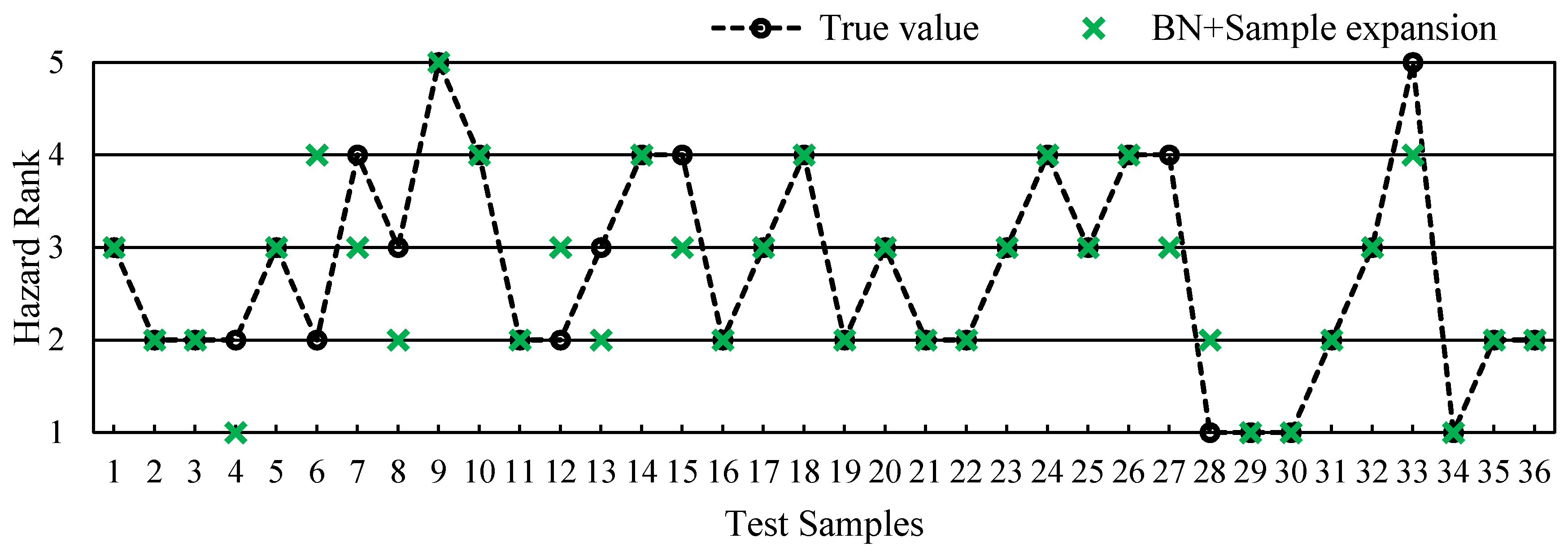
(1) Sample expansion vs. Sample non-expansion

In order to verify the effectiveness of sample expansion, we use the data sets before and after the sample expansion to construct two different BN-based evaluation models. The assessment results of marine disaster hazard with testing samples are illustrated in Figure 3.

It can be seen from the figure that the BN trained with the original sample (sample size is 50) has a large deviation between the evaluation and reality, and the prediction accuracy of the hazard level is only 56.67%. With the BN trained with expanded samples (sample size is 550), the evaluation accuracy is up to 90.11%, increased by 33.44%. It demonstrates that the expanded samples based on the information diffusion algorithm effectively extract the data structure information from limited samples, improving the performance of BN. The sample augment method provides a technical approach for disaster assessment in a data-scarce environment.

(2) BN vs. BPNN and ELM

In order to verify the effectiveness of BN, based on the expanded samples, we use BN and two, frequently used machine learning (ML) algorithms, Back-Propagation neural network (BPNN) and extreme learning machine (ELM), to build different hazard assessment models and compare their assessing performance. In modeling with BPNN and ELM, the number of network layers is three in both cases.

Figure 4 shows the assessment results of three models. The prediction accuracy of BPNN and ELM are 73.34% and 76.67%, respectively, which are significantly lower than the accuracy of BN (90.11%). More importantly, BPNN and ELM are ML algorithms with deterministic outputs, and the assessment results are single certain value, which cannot handle and express the uncertainty in disaster assessment. In contrast, BN not only obtains high accuracy in evaluation and prediction with mining the influence relationship among indicators, but also can deal with uncertainty through the probabilistic reasoning.

(3) Information Diffusion vs. Bootstrap

In order to further illustrate the effectiveness of the sample expansion based on the information diffusion algorithm, we compare it with the most commonly used sample expansion algorithm, Bootstrap, also known as the self-service statistical method.

The Bootstrap algorithm is a statistical method for expanding samples [34]. Its core idea is to use the distribution of samples to simulate the statistical characteristics of the unknown probability distribution, and then obtain approximate location parameters. The small samples are expanded by the information diffusion algorithm and Bootstrap algorithm respectively, and then different BN-based assessment models are constructed based on the two expanded samples. Figure 5 shows the evaluation results.

It can be seen from the figure that the BN trained with expanded samples from the information diffusion has the highest prediction accuracy (90.11%); the expanded samples with the Bootstrap algorithm can slightly improve the probabilistic reasoning accuracy of BN (72.23%), which is obviously lower than that of information diffusion. We also use BPNN and ELM to carry out the same evaluation and prediction experiments, as shown in

Table 12. Assessment accuracy of different models.

	BN	BPNN	ELM
Sample non-expansion	56.67%	46.67%	51.21%
Bootstrap	72.23%	63.34%	66.67%
Information diffusion	90.11%	73.34%	76.67%

.

For BN, BPNN and ELM, the samples expanded by information diffusion result in greater improvement of assessing performance than the Bootstrap algorithm, indicating that the information diffusion algorithm can effectively extract and expand the data structure information from incomplete limited samples. Our proposed model provides a solution to the hazard assessment with small samples.

(4) Generality Test

Generalization ability is usually known in the ML community, used to describe the algorithm’s adaptive capacity to new samples. In order to test the generality of our proposed model, we input different testing samples into the BN-based assessment model established in Section 4.3. Environment and disaster data from another time period (April to November of 2001–2005) are selected as new testing samples to verify the performance of the model. The results in Figure 6 show that the accuracy has dropped. This is because BN only learns the patterns from training samples (2005–2019) while the rules of new testing samples (2001–2005) are not captured. The new testing samples are different from training samples in statistical rules, so the assessment accuracy decreases. However, it is up to 80.56%, still better than BPNN (73.34%) and ELM (76.67%), indicating that the assessment model has the characteristic of general use.

5. Conclusions

There are two challenges in the studies about the comprehensive hazard assessment of marine disasters. On the one hand, interactions between each two indicators are non-linear, and the impact mechanism between indicators and disaster hazard is fuzzy. On the other hand, time series of disaster data are not long enough, and the continuity is poor, especially in the lack of associated information between disaster losses and environmental conditions. To solve the two problems, we combine the information diffusion algorithm and BN to put forward a novel assessment model, coming with two advantages:

(1) Sample expansion. The information diffusion algorithm is used to expand associated samples between disaster losses and environmental conditions so that sufficient disaster data can be obtained for model construction.

(2) Uncertainty expression and reasoning. BN is capable of mining influence relationships among the marine hazard and environmental factors through structural learning and parameter learning. Based on the probability theory, BN achieves the expression and reasoning of uncertain relationships.

Experimental comparison results show that our proposed model is able to deal with the uncertainty relations and achieve more accuracy risk assessment under the small sample condition. However, in the practical application to some coastal areas, there may be a serious lack of data on some indicators. Extreme data loss may affect the efficiency and feasibility of information diffusion algorithm. In addition, BN learning is the core of the proposed assessment model. The richness of training data sets can affect the application range of the model. Besides this, the BN structure is established based only on objective data in our research. However, studies show expert knowledge can also improve BN learning [35]. Therefore, we will focus on improving the structural learning and parameter learning of BN in the next step.