1. Introduction
Recently, the demand for AIS (Automatic Identification System) data for research and development in the maritime transport discipline has been continuously increasing [
1]. AIS enables ships to communicate with each other or contact satellites and base stations using various information such as a Maritime Mobile Identification Number (MMSI), longitude, latitude, speed over ground (SOG), course over ground (COG), headings, etc. [
2]. Researchers have found that AIS can function as a big data source not only for maritime safety but also for other kinds of research, such as traffic analysis, transport economy, emissions, etc. [
3].
Although AIS has played a significant role in maritime transport-related research with its enormous amount of data, data error is likely to occur due to various factors [
4,
5]. Those incorrect data lead to inaccurate conclusions in trajectory analysis, which is crucial for further applications. Therefore, it is of great concern to detect and remove those abnormal data to improve the quality of AIS data.
To date, researchers have made great efforts to identify abnormal data in AIS through different methods. According to [
6,
7], the abnormal data detection methods for ship trajectory can be divided into two types: knowledge-driven and data-driven. In general, those methods that correspond to the knowledge-driven approaches can be regarded as rule-based methods. The simplest way to conduct anomaly detection for AIS data is to use a predefined data range to determine and exclude the outliers [
8], which is efficient but has relatively poor performance in terms of its accuracy and reliability. In [
9], the authors considered the geometric shape of a ship trajectory and proposed a vector-based method to detect anomalies. Besides, since AIS data can describe the kinematic characteristic of a ship, based on the nearly-constant velocity (NCV), an Ornstein–Uhlenbeck model has been proposed to detect whether a ship deviates from a planned route [
10]. Apart from the single factors such as the shape characteristic of ship trajectories, factors such as position, speed, acceleration, rate of turn, etc. can be used to discover abnormal data [
11,
12] following some pre-defined criteria for the anomaly. However, the drawbacks of this kind of approach are obvious: the definition of the rules relies on human knowledge and the characteristics of the regional data, and thus it is difficult for this approach to provide a generalized anomaly detection method.
Different from the knowledge-driven approaches, the data-driven approach focuses on learning the ship behaviors from the trajectory data to generate motion patterns. Those behaviors that differ from the extracted patterns are considered anomalies, the associated data will then be detected. Based on the way to extract motion patterns, the data-driven approaches can be further divided into three kinds: Similarity-Based, Supervised-Learning-Based, and Unsupervised-Learning-Based. For Similarity-based methods, the similarity between the trajectories is applied as an alternative to determining the anomaly of the trajectory by comparing it with all labeled trajectories. A common challenge in similarity calculation is the unequal length of different trajectories, and thus a varies of methods have been proposed to overcome the issue [
13]. A method based on Hausdorff distance is proposed by [
14] to compare the similarity of multi-dimensional trajectories and detect the abnormal in them. Reference [
15] proposed a method of asynchronous trajectory matching based on piecewise space-time constraints (PTSCTM) to reconstruct and discover the anomalies of ships, in which the Euclidean distance and time distance are used to find similar trajectories points.
However, when the scale of the dataset increases, using similarity becomes impractical as all the labeled trajectories have to be considered whenever a new trajectory is included. With the rapid development of artificial intelligence, machine learning is widely used to analyze and learn patterns from data. The supervised-learning-based method learns the mapping relationship between trajectory data and motion patterns that have been utilized in the anomaly detection of a ship’s AIS trajectory. A model using the Received Signal Strength Indicator (RSSI) and One-Class Support Vector Machine (SVM) is proposed in [
16] to detect anomalies in AIS and further identify intentional AIS on-off transitions. In [
17], the authors used hierarchical and k-medoids to learn typical ship navigation patterns and adopted the Naive Bayes classifier to detect anomalous ship behavior.
Different from supervised learning, in many situations, when given a set of inputs, the output is not specifically defined. When the motion patterns of the trajectory are not well defined, the Unsupervised-Learning-Based approaches play an important role. Reference [
18] the combined topic model with a generic algorithm to calculate the anomaly probability of a new trajectory. An unsupervised model called Traffic Route Extraction and Anomaly Detection (TREAD) is establish in [
19] to automatically learn maritime traffic patterns. To reduce the training time, the water area is partitioned in [
20] to establish a training framework based on Adaptive Kernel Density Estimation (AKDE). The combination of Supervised-Learning-Based and Unsupervised-Learning-Based methods results in a hybrid approach. This complementary method is often used as a predictor to discover anomalies. Reference [
21] applied Density-Based Spatial Clustering of Applications with Noise (DBSCAN) to obtain traffic patterns which will be then used to train a Recurrent Neural Network (RNN) to predict the trajectory for anomaly detection.
In general, the data-driven approach is simple to conduct as it does not require much knowledge from experts to build the model. However, these methods need a large amount of training data to establish a sophisticated model, and the quality of the training data directly influences the performance of the anomaly detection. To overcome the drawbacks of knowledge-driven and data-driven approaches and to establish a model that can efficiently identify the abnormal data in AIS data sets, this paper provides another perspective on anomaly detection; i.e. identifying anomalies of ship trajectory data based on the kinematic characteristics of the ship—its speed and course information. By comparing the estimated data according to the motion characteristics of the ship and the original data, the anomalies in the trajectory data can be identified using the clustering technique. Compared with the existing methods, the main contributions of this work are as follows: (1) we make full use of longitude, latitude, SOG, and COG information in AIS to estimate the reference AIS data based on the kinematic characteristics of the ship; (2) we introduce a clustering method to identify abnormal data by comparing the original data and the kinematic-based estimation. With this design, the proposed method can be of great practical value as it does not require a large amount of expert experience or training data with high quality. It should be noted that, although missing data also correspond to abnormal data, as they do not exist in the obtained dataset and can be restored by other reconstruction methods [
22], they are not considered in this paper. With the improved effectiveness of the anomaly detection of AIS data, the proposed method would facilitate AIS-based research and development in the maritime transportation industry, such as for maritime traffic management, Maritime Autonomous Surface Ship (MASS), autonomous collision avoidance, etc.
The rest of this paper is structured as follows:
Section 2 presents the methodology used in the research, followed by details of the designed models in
Section 3. A case study including several types of trajectories is presented in
Section 4, together with further discussion on the performance of the proposed method, with a comparison between the rule-based anomaly detection approach.
Section 5 concludes the research and presents possible directions for improvement.
3. Model Design
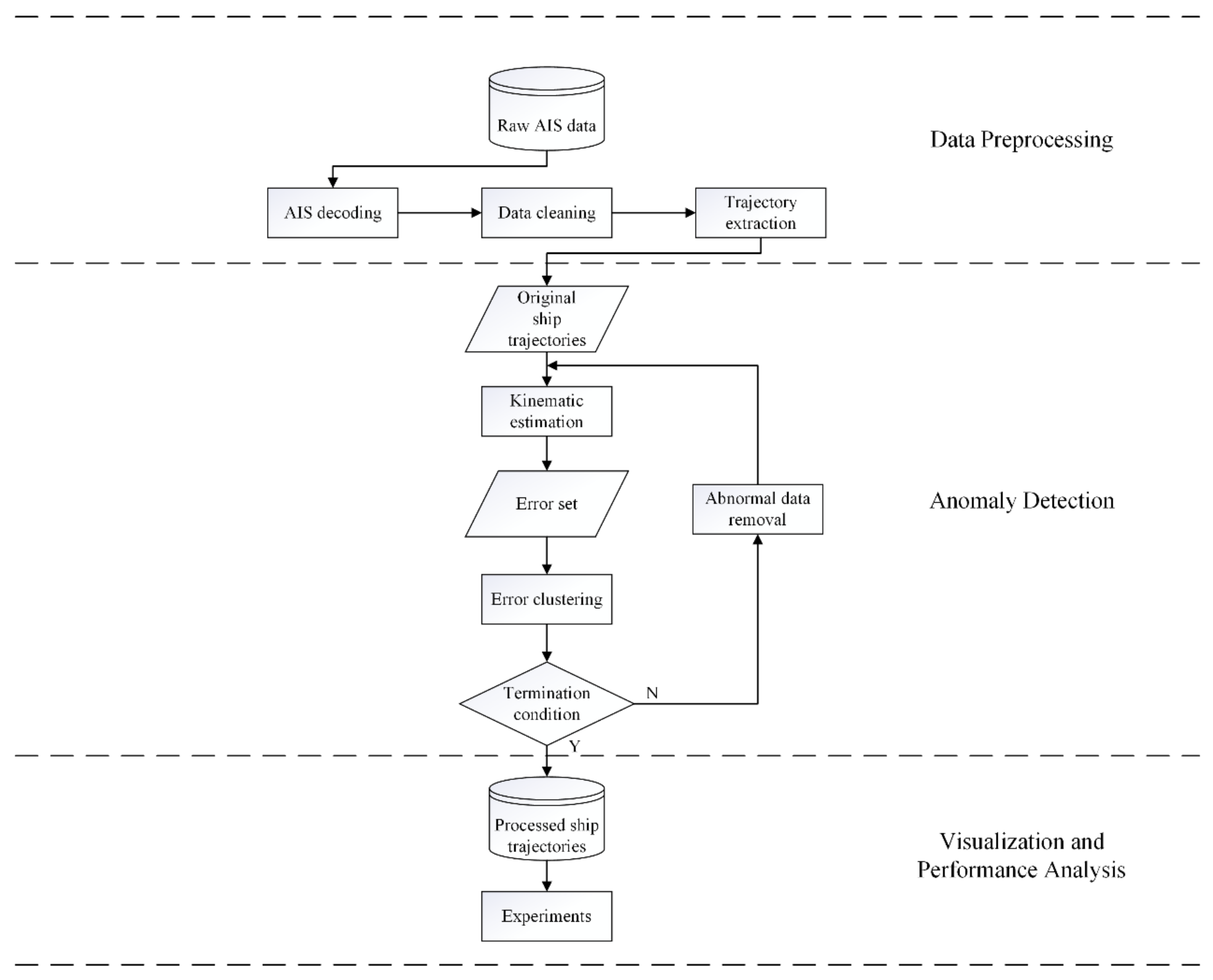
The objective of this research is to propose a new anomaly detection method for ship trajectory data from the perspective of the kinematic characteristics of ships. To achieve this objective, three major components need to be developed, which are as follows: (1) a kinematic estimation model for AIS data, (2) an anomaly detection model based on the kinematic estimation model, and (3) an iterative detection model based on loop detection with a termination condition. This section describes the models utilized in this method in detail.
3.1. Kinematic Estimation
The kinematic estimation of AIS data is conducted to estimate the data points of a ship trajectory according to their kinematic characteristics, such as velocity and course, etc. The objective of this procedure is to provide a reference point to determine if the trajectory data follow the kinematic characteristics of the ship. To conduct this operation, the definition of the trajectory should be first introduced.
For the ship trajectory data set , the definition for the trajectory in is described as follows: , where indicates the name of the ship to which belongs, and is the trajectory points set of the trajectory . For the point in , , where represent the timestamp, longitude, latitude, SOG, and COG of , respectively. denotes the number of points in . The details of the anomaly detection of the AIS trajectory are elaborated in the following sections.
To attain our objective, we introduced a sliding window method to the trajectory to calculate each estimated point using the kinematic interpolation method. The principle of the method can be seen in
Figure 3. The size of the window was set to 3 (w = 3), containing two endpoints and a mid-point.
As the window slides, an estimated point corresponding to each trajectory point is produced with the kinematic interpolation method. Please note that in Equation (1), we mainly use three kinds of kinematic information—position, velocity, and acceleration—at certain times. However, AIS trajectory data do not contain acceleration information. The solution to this is to introduce the linear motion characteristic suggested in [
27] based on the frequency characteristics of ship AIS trajectory data, which is shown in Equation (2):
where
is the acceleration of a ship at time
;
is the time of the estimated point;
is the time of the start point; and
and
are two parameters to be determined with the data. It should be noted that Equations (1) and (2) only consider the moving object in one dimension. For a trajectory point
, its positions in longitude and latitude directions are known as
and
, and the velocity can also be determined based on Equation (3):
To simplify the following description, we only illustrate the formulas in one dimension; the other dimension can be determined in the same manner. Equation (1) can be rewritten as Equation (4) with the integration of Equation (2):
If the start point and end point are
and
, the parameters
and
can then be solved by substituting their positions and velocities into Equation (4), which is shown in Equation (5):
Once
and
are solved, the object’s status at any given time
can be estimated by Equation (4).
3.2. Anomaly Detection of AIS Data based on Error Clustering
As mentioned above, the principle of this research is to identify an anomaly in ship AIS data considering the kinematic characteristics of the data. To achieve this objective, the kinematic estimation is first applied to provide a reference for the verification of the data, based on which the error between the estimated data points and AIS data are analyzed to determine the anomaly in the data sets. The details are presented below.
3.2.1. Error Calculation and Error Weight
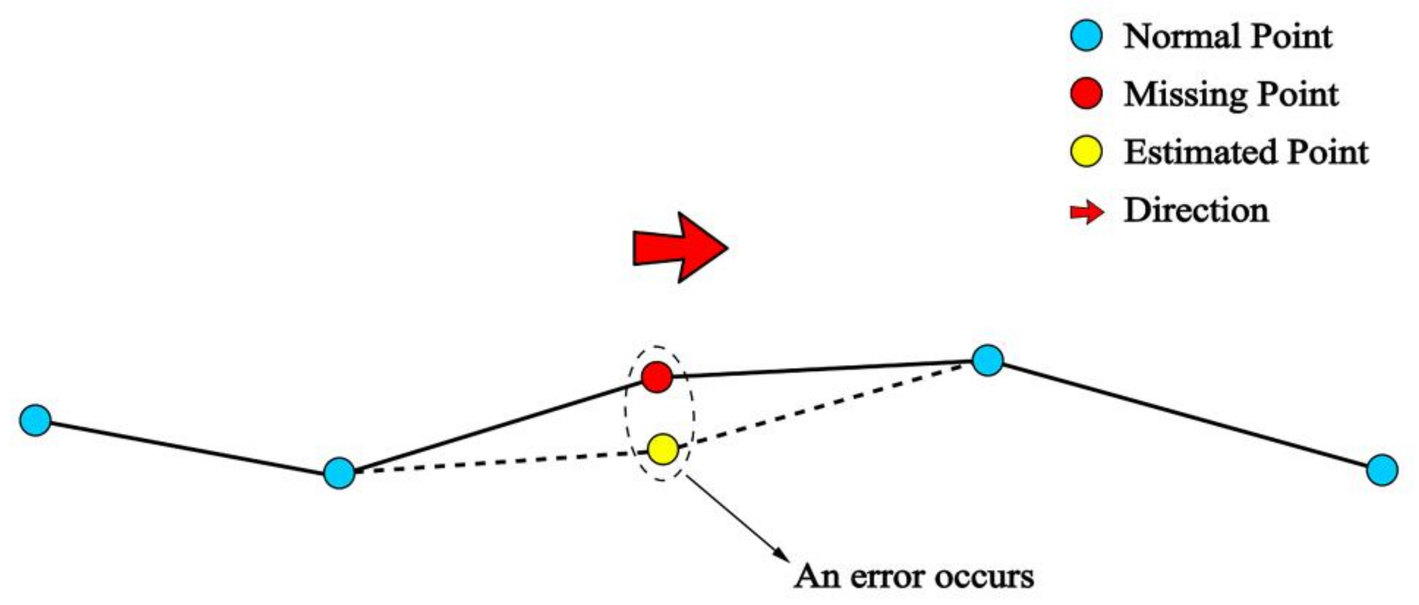
When the sliding window process is complete, one can see from
Figure 3d that, except for two endpoints, each datapoint has a corresponding estimated point. If there is no error in the trajectory data, the estimated point should be close to the known points, but when there is any error in position, velocity, or direction, the estimated point will be far away from the known point. The principle of the error estimation process for the trajectory points is shown in
Figure 4.
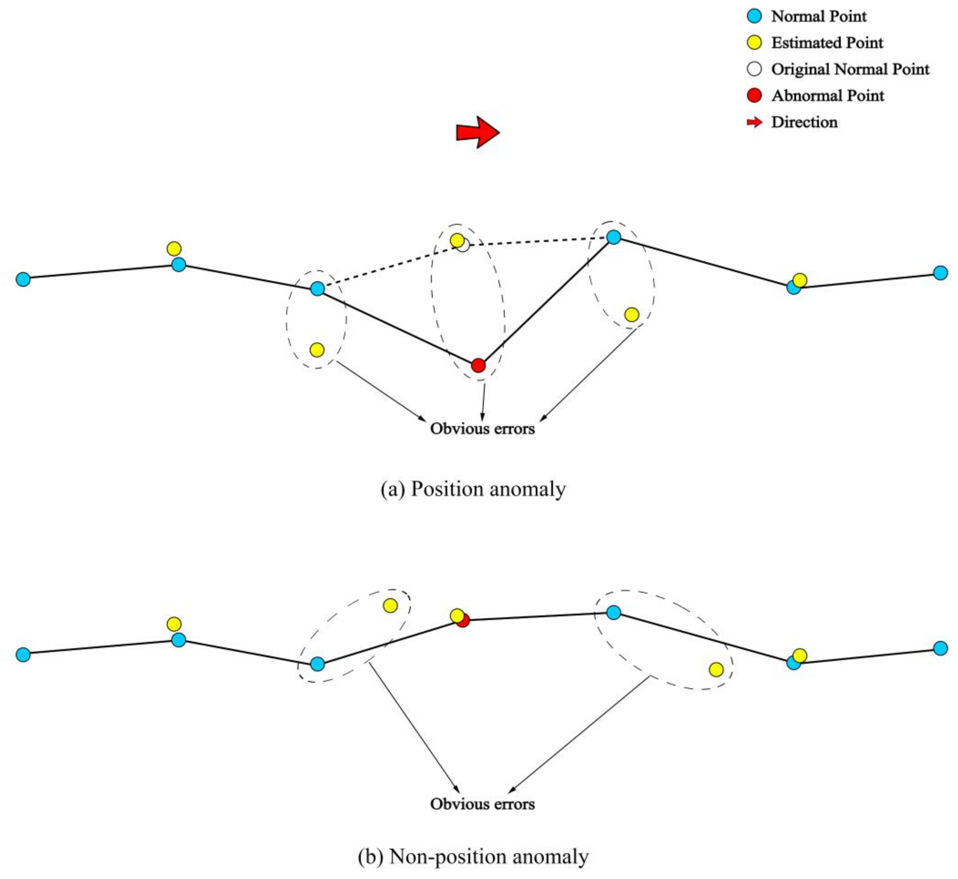
In
Figure 4a, one can see that when a position anomaly occurs, three continuous estimated points show obvious errors. As shown in
Figure 4b, the abnormal data containing velocity errors are difficult to identify from the positioning perspective, as their position information is correct. To identify this anomaly in its velocity perspective, the error between a trajectory point
and its accompanied estimated point
should be estimated with the integration of velocity information following Equation (6):
where
denotes the distance between
and
using the Mercator projection method, and
denotes their velocity difference.
Since
can be used up to three times to calculate the relevant estimated points during the sliding window process, we introduce an error set
to denote relevant errors of
.
with this design, the error weight
for the data point
can be calculated as shown in Equation (8):
where
has the same setting as that in
, and
is the number of elements in
, which indicates how many times
has been used to calculate the errors. Thus, each point has an error weight value. The error weight set can be denoted as Equation (9) shows:
As mentioned above, the errors in the position and velocity of the AIS data are all considered in the anomaly detection model. Using this design,
contains two kinds of values, which is the errors in position and velocity. Their dimensions are different, which are
and
. To obtain an accurate result for anomaly detection, first, we need to eliminate the influences of dimension and order of magnitude. Therefore, a standardization process is applied to
:
where
and
are the mean value and standard deviation of
,
is the standardization result of
, and
is the standardization weight set.
3.2.2. K-Means Clustering and Anomaly Detection
In the prevision section, an error estimation method was proposed based on the kinematic information of ship AIS data to provide a reference for the anomaly detection from the ship kinematic perspective. The next step is to propose a method to identify which data points are abnormal based on their error estimation. As a widely used clustering method, K-means can detect abnormal data effectively. In this section, we illustrate the details of utilizing an improved K-means clustering approach to identify an anomaly in an AIS data set.
First, for the number of clusters, a trajectory point can be used up to three times in the sliding window process to obtain the error weights of . In this case, there are four possibilities when determining an anomaly in the data: (1) no anomaly occurs, (2) an anomaly occurs once in the error weights, (3) two anomalies occur in the error weights, and (4) three anomalies occur in all three iterations of the error calculations. Thus, the number of clusters can be determined as 4.
For the clustering of the error weights of the AIS data points, in this research, we adopt an improved method called K-means++ [
31]. The principle of K-means++ is to ensure the distance between the initial clustering centers is as far as possible, which can reduce the influence of the selection of the initial clustering center on clustering results. Finally, the noise and outliers can be automatically detected with the proposed clustering method. A short example of this method is shown in the following section.
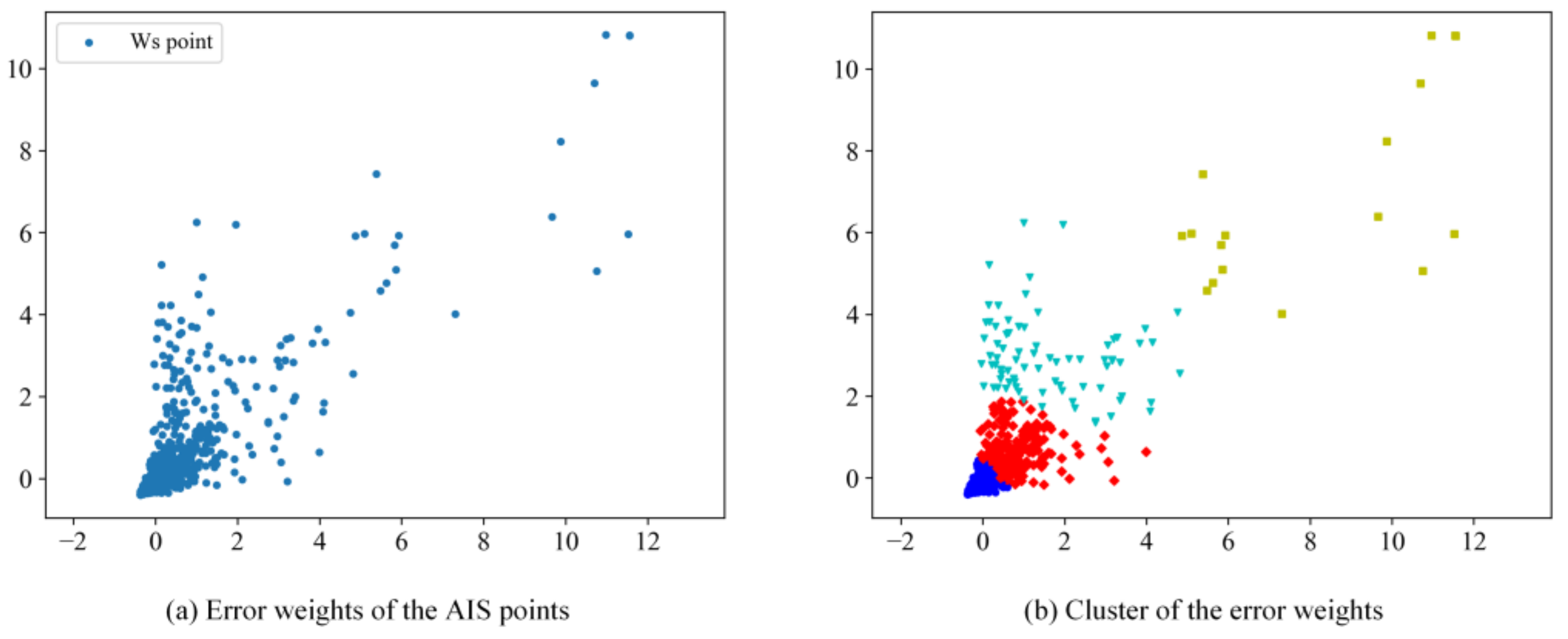
Figure 5a shows an illustration of
for a randomly chosen trajectory. By adopting the K-means clustering method on
, points in
Figure 5a can be divided into four clusters, as shown in
Figure 5b. If a point
is not abnormal, then
should be as close to (0, 0) as possible in the coordinate system; otherwise, the further it is from (0, 0), the higher the possibility that
could be an anomaly. One can see in
Figure 5b that the red diamond points are far away from (0, 0); points with these standardization weight values have been identified as abnormal data, indicating that each of them has anomalies in all three calculations in the kinematic estimation. In this way, the most likely abnormal data can be detected, and the point set relevant to the farthest clusters to (0, 0) is defined as
.
3.3. Loop Detection and Termination Condition
Since an improved K-means clustering method is applied on , it is possible to identify the most abnormal data in a trajectory. However, some hidden anomalies might be omitted from the detection. To detect them all, a further step is necessary. Here, we introduce a loop detection process, which is implemented to detect all abnormal points in trajectory data by the repetition of the kinematic estimation and error clustering process.
Within the data set,
can be influenced by the neighbors of
, as
can be normal but its neighbors abnormal. For the detection process, an abnormal data set
is established with the clustering process. The data points in this cluster are removed in one iteration of the error clustering process. Then, the point set of
changes to
. Let
, which indicates the initial number of points in the original trajectory data set; the definition of
is shown in Equation (11):
where
is the current number of loops,
is the trajectory point set before the current loop’s start,
is the abnormal point set detected in the current loop, and
is the trajectory point set after the current loop. When the loop detection is terminated, let
, which indicates the final number of points after the anomaly detection process.
The termination condition of this process is set as follows: Considering the final state of the anomaly detection, the trajectory
should have no abnormal data in
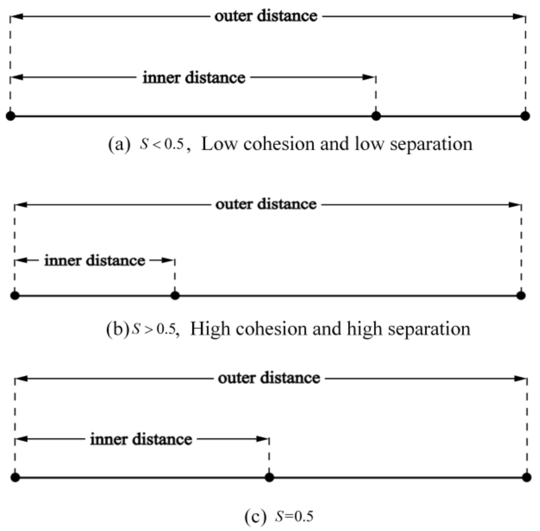
. From this perspective, we utilize the performance of the clustering as the criteria to determine when the loop can be terminated; i.e., if the clustering shows good performance with only one cluster, that would mean the abnormal data have been identified and removed from the trajectory. To describe the performance of our approach, we introduce the silhouette coefficient, which was first proposed in [
32]. The silhouette coefficient is defined as follows:
where
is the average distance between
and all other points in the cluster to which
belongs.
is the average distance between
and all points in the nearest cluster. To make this easy to understand,
and
can be understood as the inner distance and outer distance, respectively. The average silhouette coefficient
is the mean value of
. The range of
S is set between −1 and 1; i.e., a higher score indicates a better clustering result.
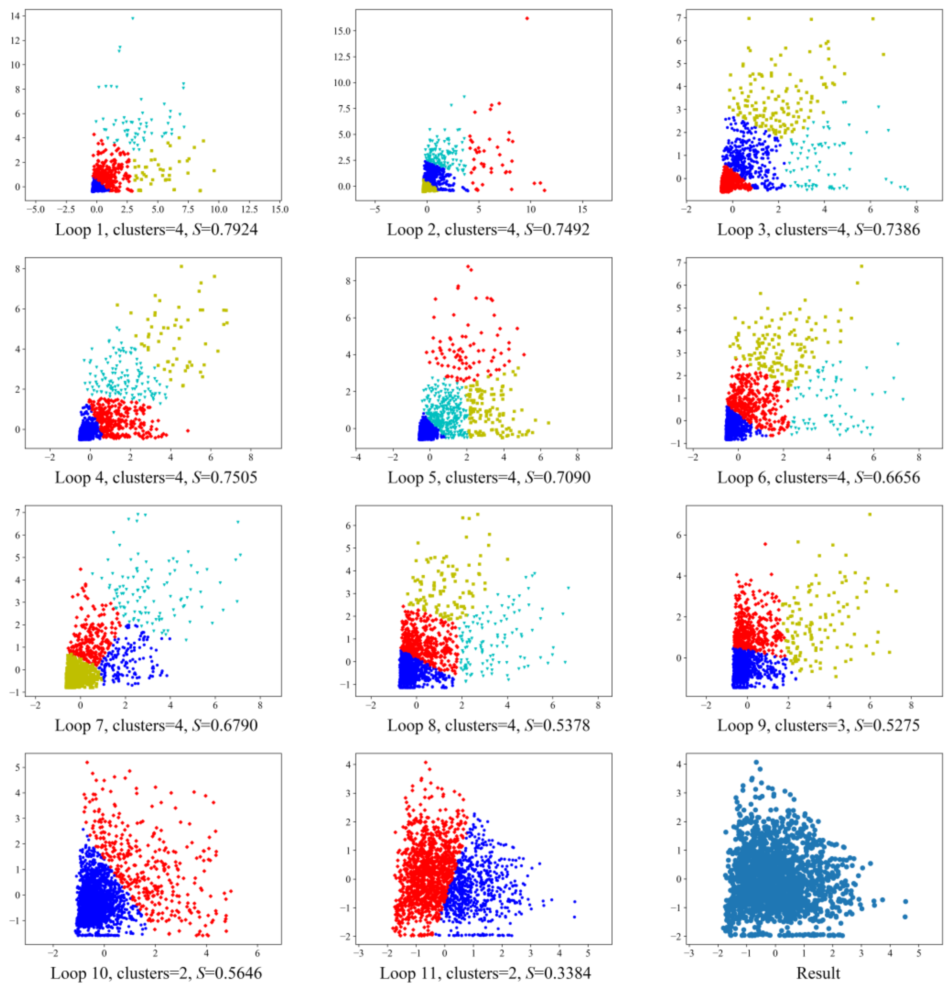
When
is lower than a certain value, denoted by
, this means that the clustering result is not good enough and is not appropriate to set the initial number of clusters as 4. This indicates that those points with the most errors in kinematic estimation have been detected and removed. For the rest of the points, if they have anomalies, the worst situation for a point is that two anomalies occur in two of the three calculations; therefore, the initial number of clusters will change to 3. From this perspective, in a detection loop, when the initial number of clusters is set to be 4, 3, and 2 in turn, if
, this means that the detection should terminate. The determination of the criteria is illustrated in
Figure 6.
When
is positive and lower than 0.5, the clustering result can be considered as low cohesion and low separation, as shown in
Figure 6a. When
is greater than 0.5, the result is considered to show high cohesion and high separation. Thus, as a critical state, we set
to be 0.5. We will not discuss the situation when
is negative, because this would mean that the result is so poor that it has to be re-clustered.
Once the termination condition is set, the anomaly detection model is completed. The pseudocode of the whole anomaly detection model is shown in Algorithm 1, followed by the design of the loop detection model in Algorithm 2.
| Algorithm 1. Anomaly Detection. |
.
# Kinematic estimation and error calculation
:
IS NOT endpoint:
);
);
AND ITS NEIGHBORS;
:
);
;
);
# Clustering
N = 4;
WHILE N != 1:
, cluster_num=N);
IF S >= Sc:
BY REFERRING TO clusters;
;
BREAK;
ELSE:
N = N − 1;
IF N == 1:
loop = FALSE;
ELSE:
loop = TRUE;
, loop; |
| Algorithm 2. Loop Detection. |
.
;
);
WHILE loop:
);
;
;
, anomaly_data; |
5. Conclusions
AIS has played a significant role in the research and development of the maritime traffic industry. However, anomalies and errors in the data have impinged on the data quality and therefore posed challenges to researchers and data scientists in facilitating this process. Therefore, as a fundamental step for the utilization and application of AIS data, it is of great significance to identify and remove anomalies and improve the data quality. In this research, a novel anomaly detection method for AIS trajectories has been proposed by integrating the kinematic information in AIS and a clustering-based method to identify anomalies in AIS data considering the kinematic characteristics of the ship.
The abnormal data in the ship AIS data set are detected by using kinematic interpolation. Using the knowledge of known trajectory points collected from raw AIS data, kinematic interpolation is used to estimate the possible errors of the original trajectory data. After the kinematic estimation and error calculation processes, the possibility of an anomaly in each point is measured with an error weight. An improved K-means clustering method is then applied to identify abnormal data by clustering the error weights of the data points. Furthermore, to achieve comprehensive detection, the error detection and clustering process is further integrated with a loop design by utilizing the silhouette coefficient as a termination condition to evaluate the performance of the clustering.
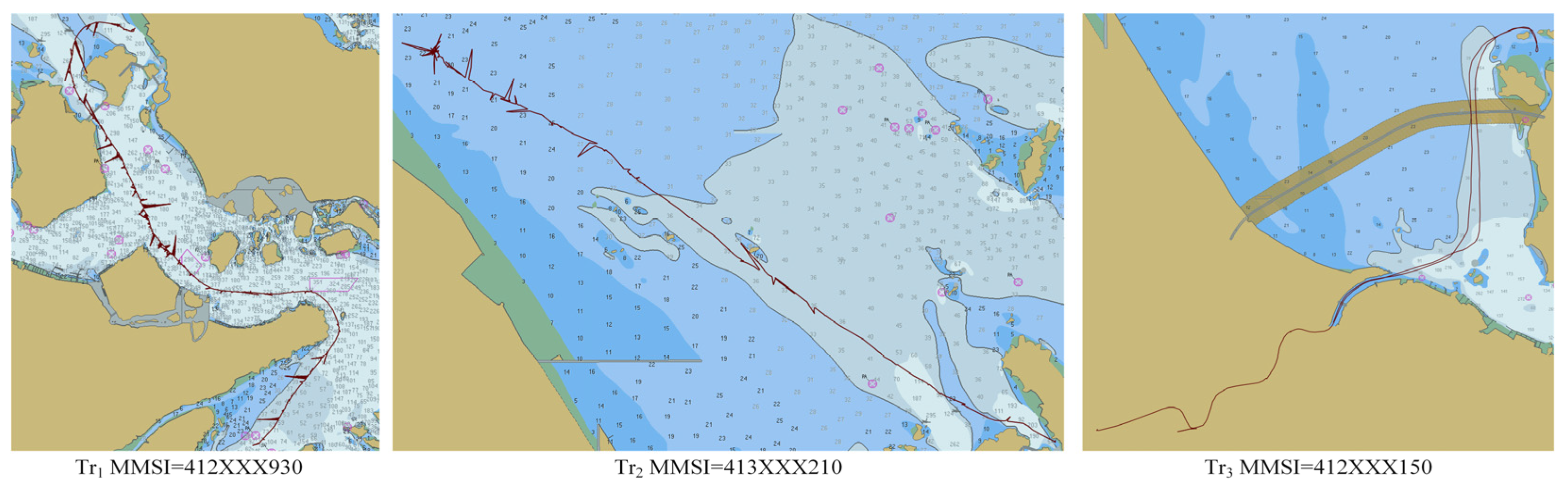
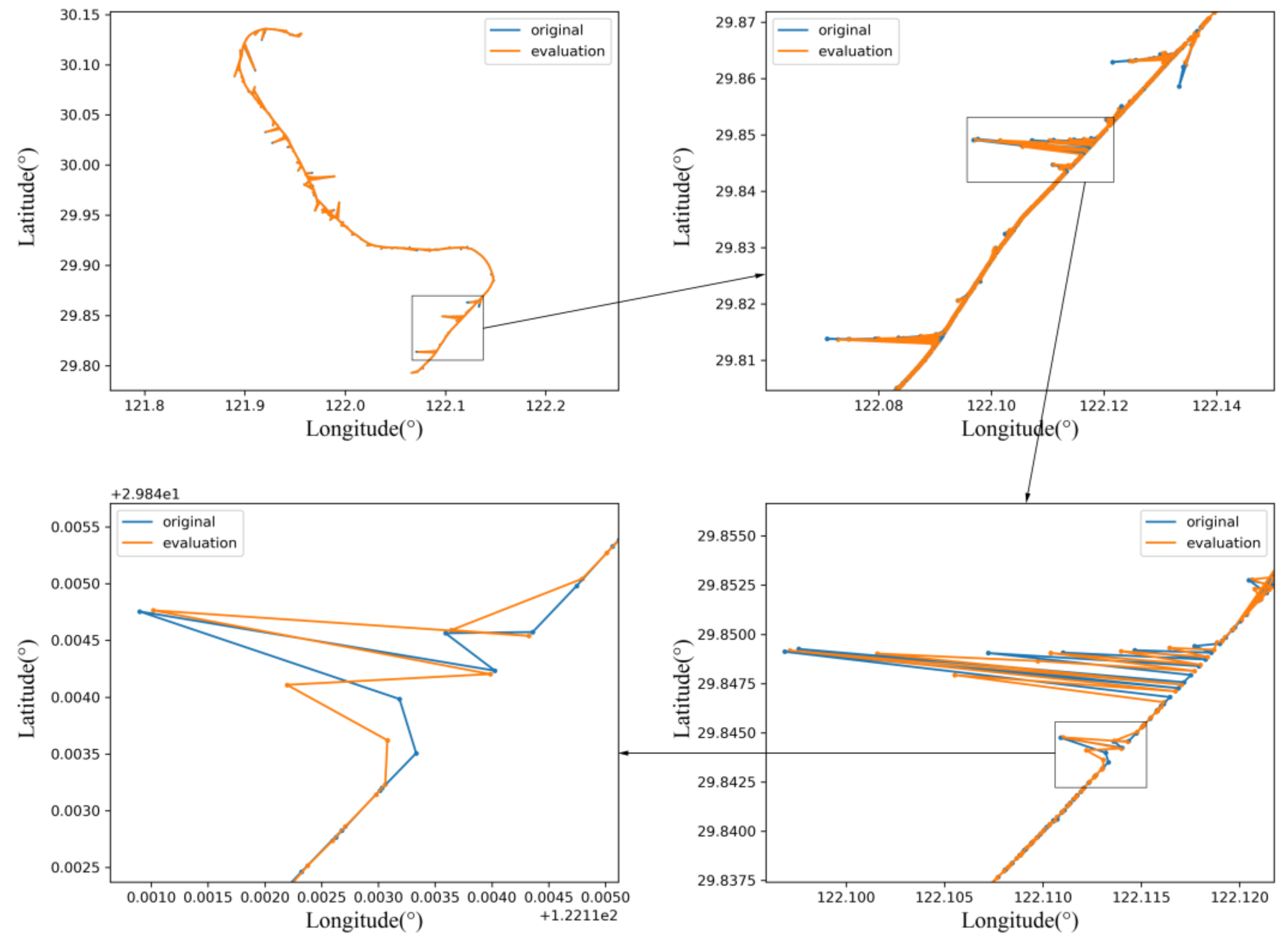
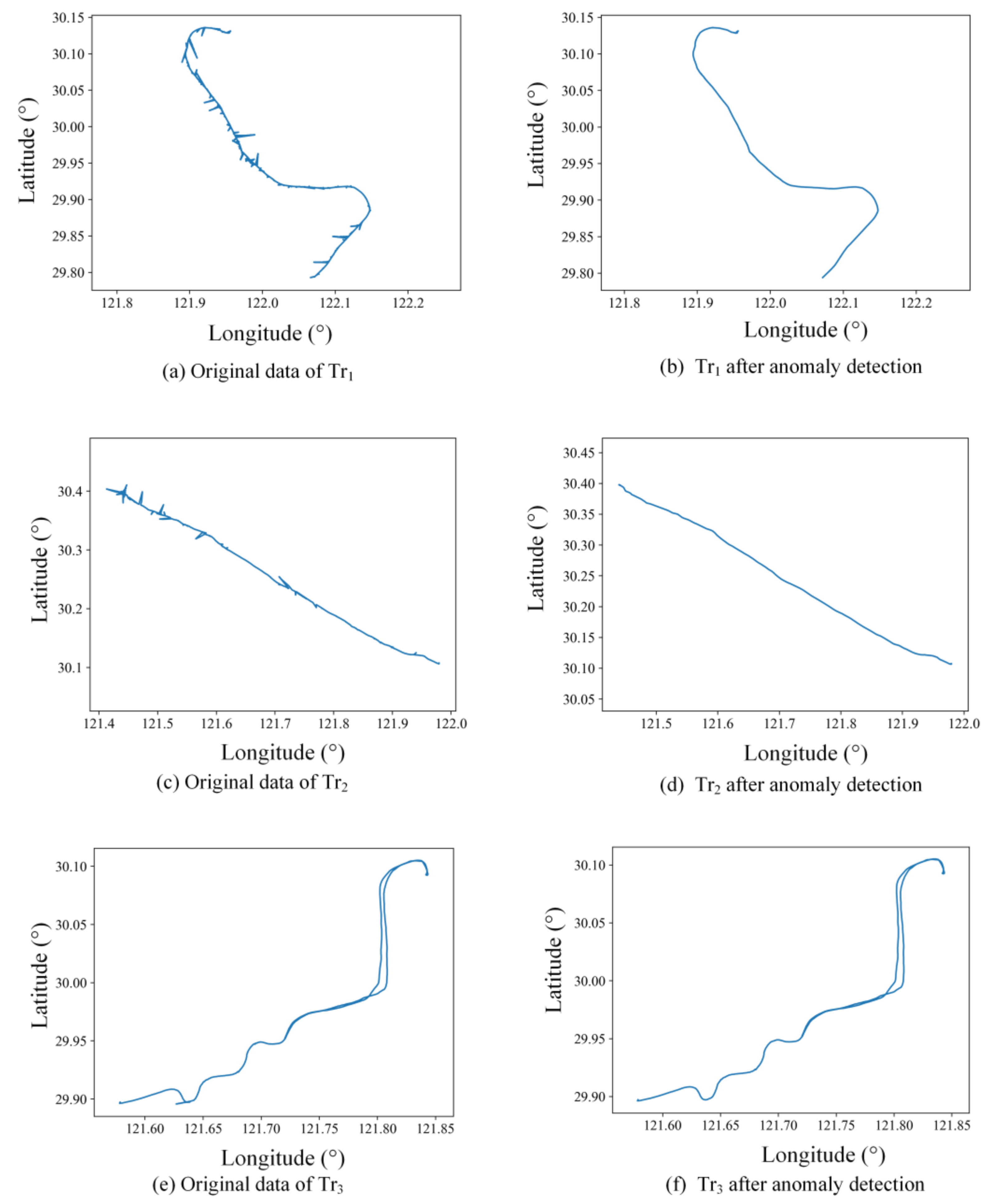
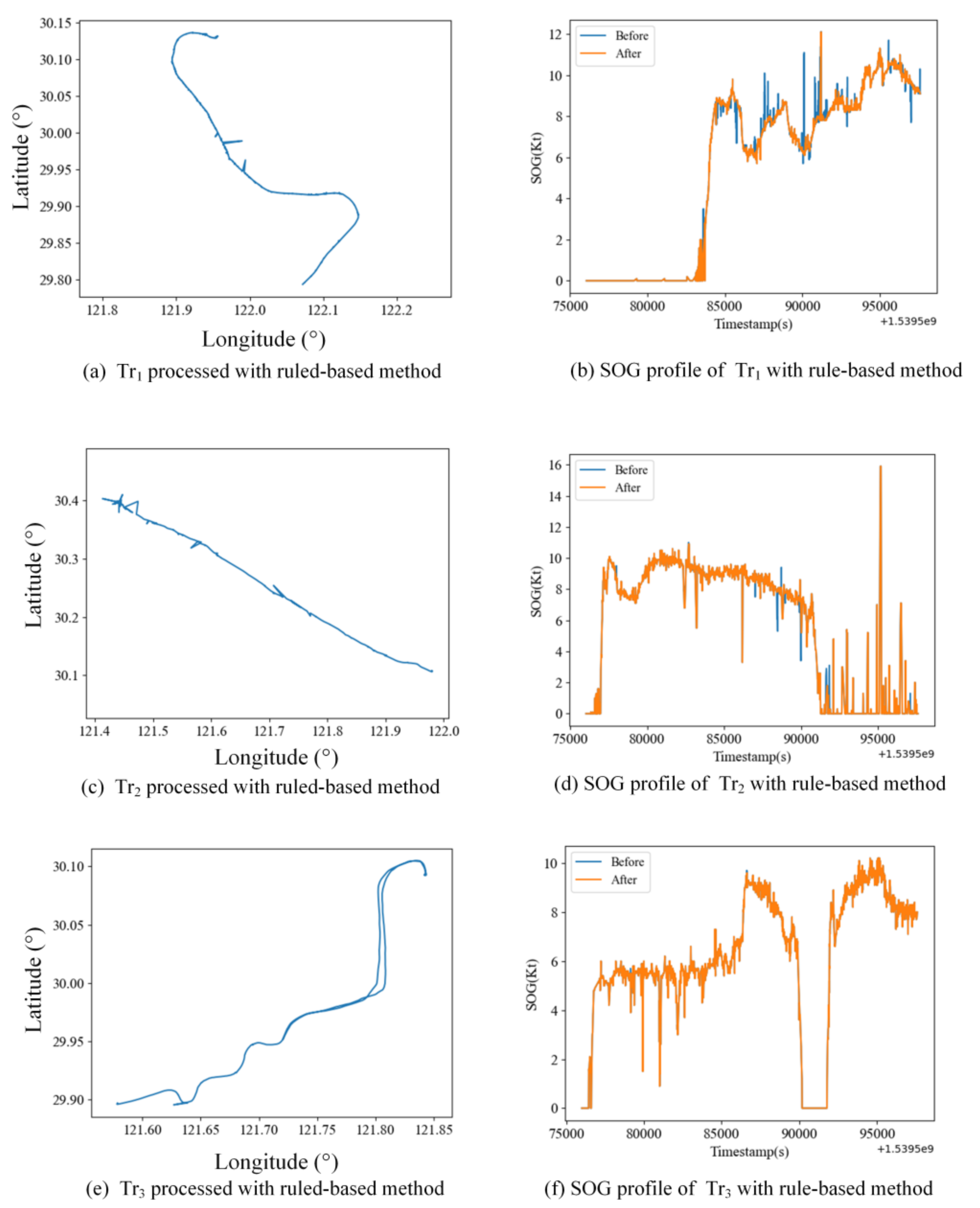
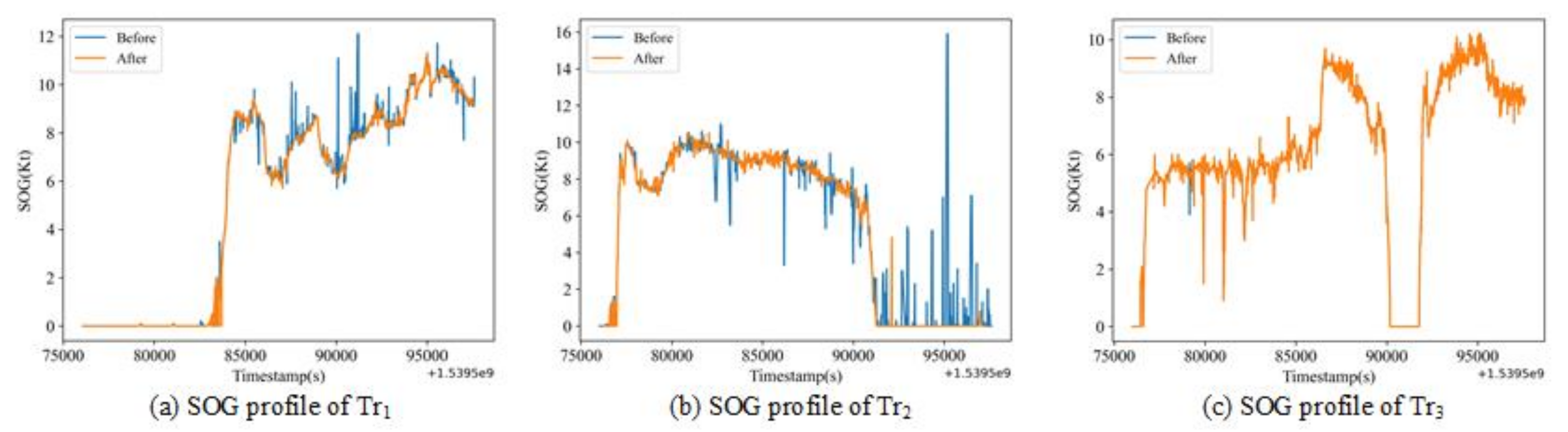
To validate the effectiveness of the presented method on different scenarios of data anomalies, a case study associated with three trajectories was conducted. From the results with kinematic estimation, one can see that the proposed method was able to successfully identify the position and velocity anomaly at the same time, showing better performance than the conventional method that only considers the problem from a position perspective. The repeated clustering process enabled the proposed method to identify all the anomalies in the trajectories and improve the data quality as much as possible. The comparison between the proposed method and the rule-based anomaly detection method indicates that, for both detailed analysis and application on large-scale data sets, the proposed kinematic-based method can identify more anomalies in both positions and speed in a data set than previous approaches.


