
Effect of Roughness of Mussels on Cylinder Forces from a Realistic Shape Modelling

 ,
,  , and
, and
Abstract
1. Introduction
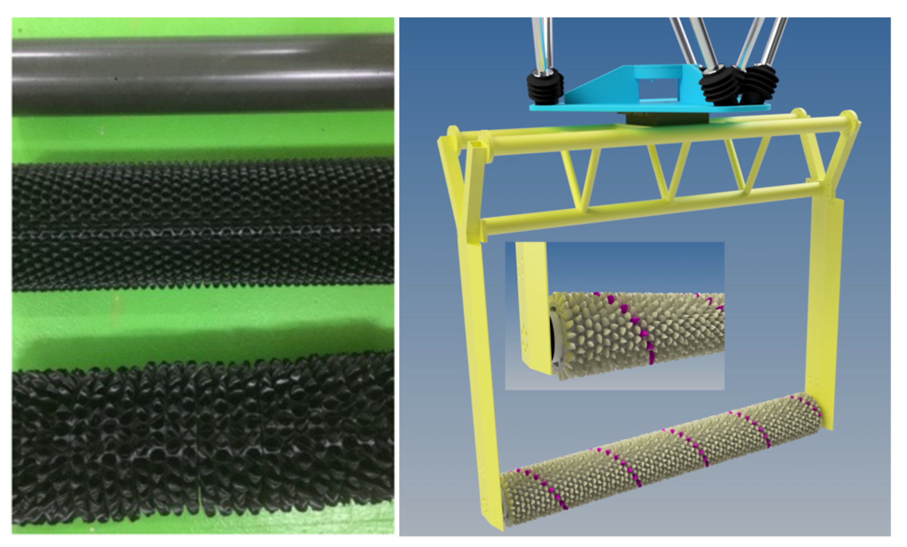
2. Hard Marine Growth Reproduction and Experimental Setup
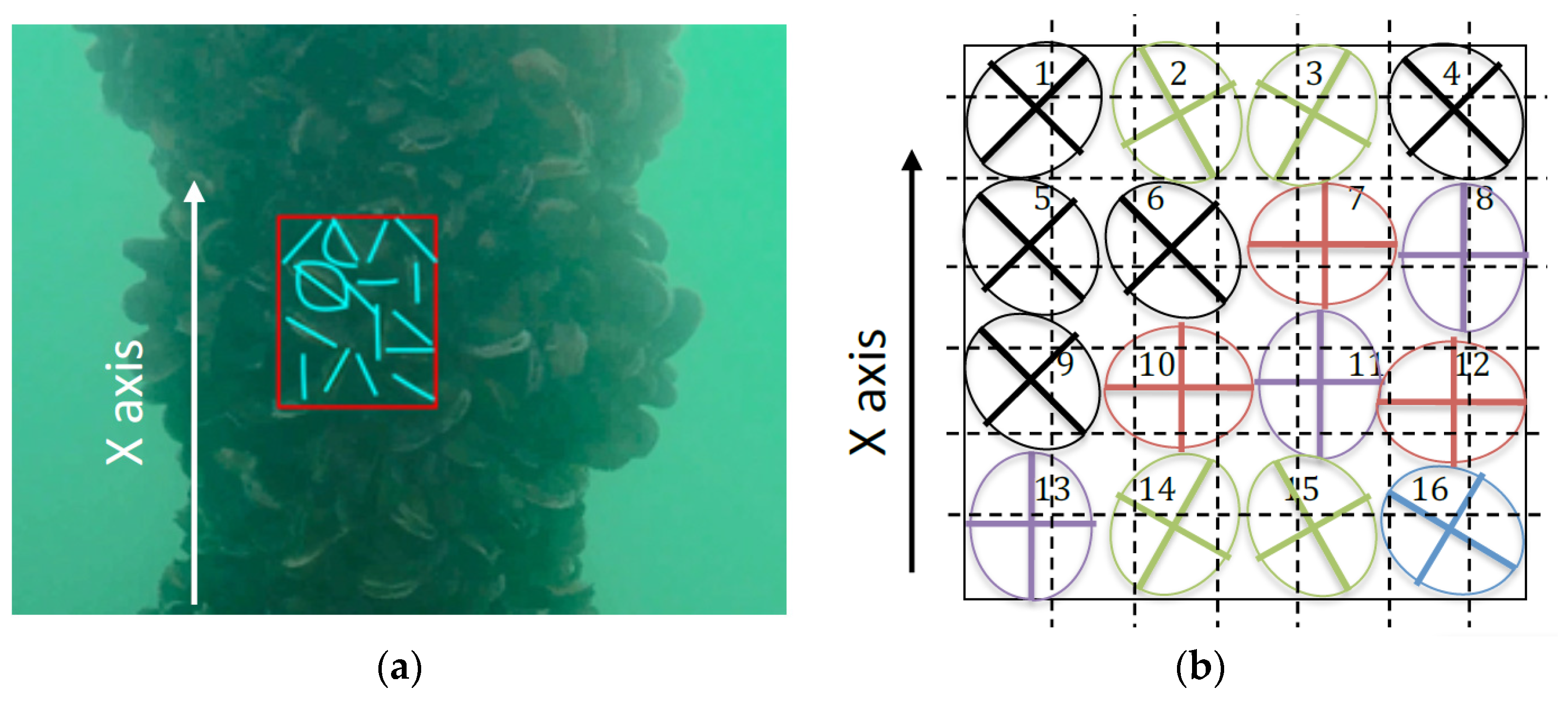
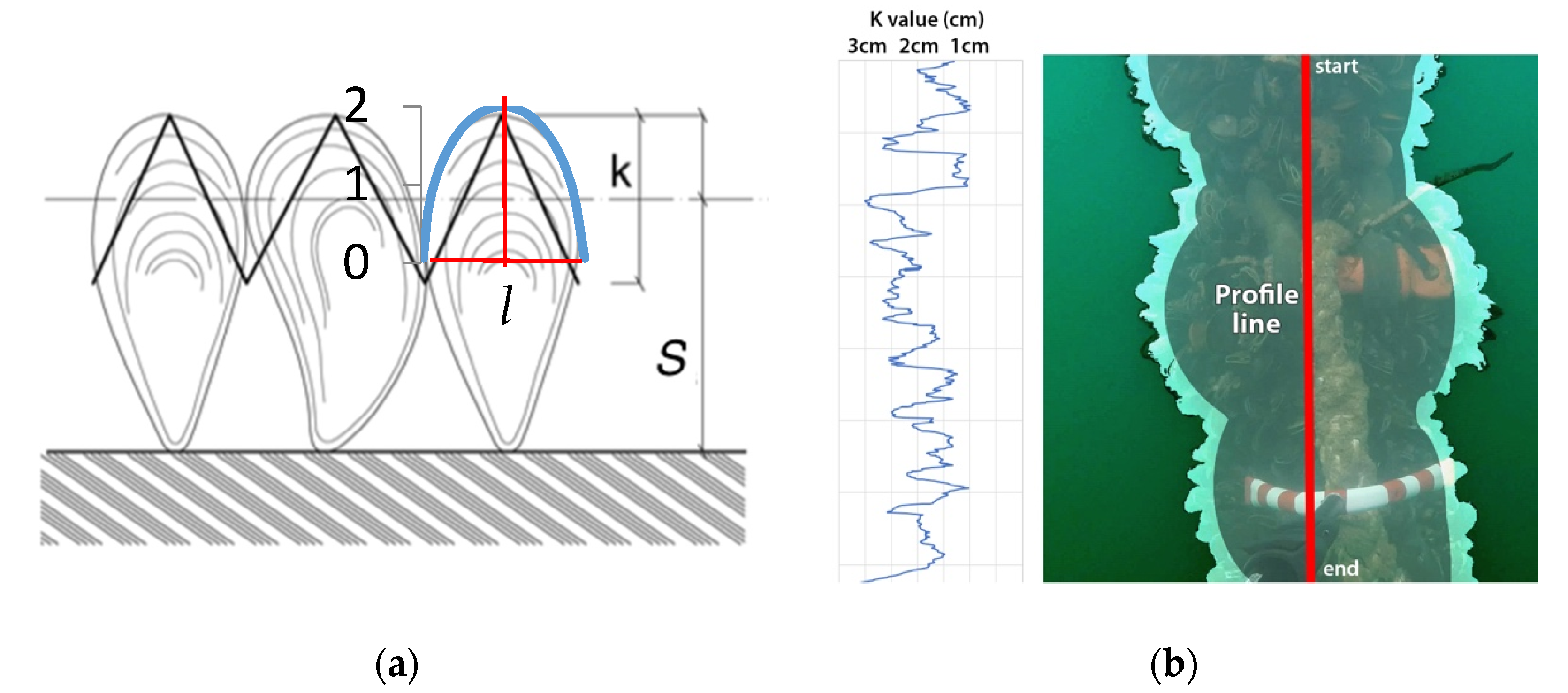
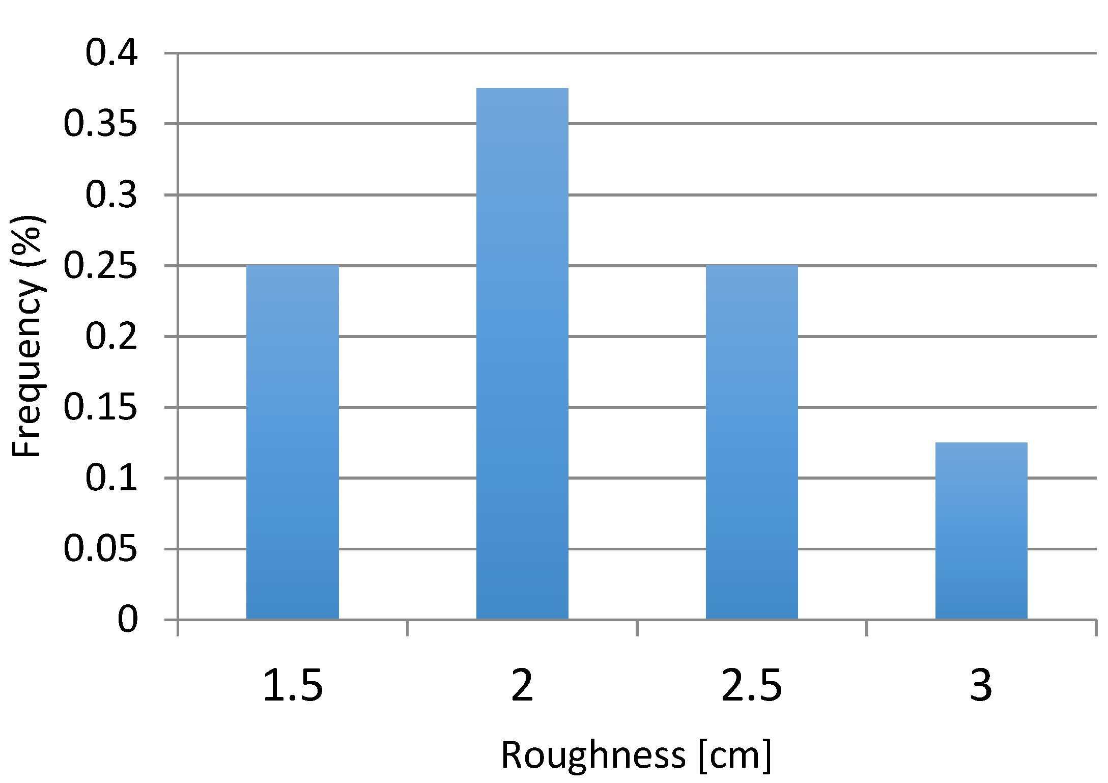
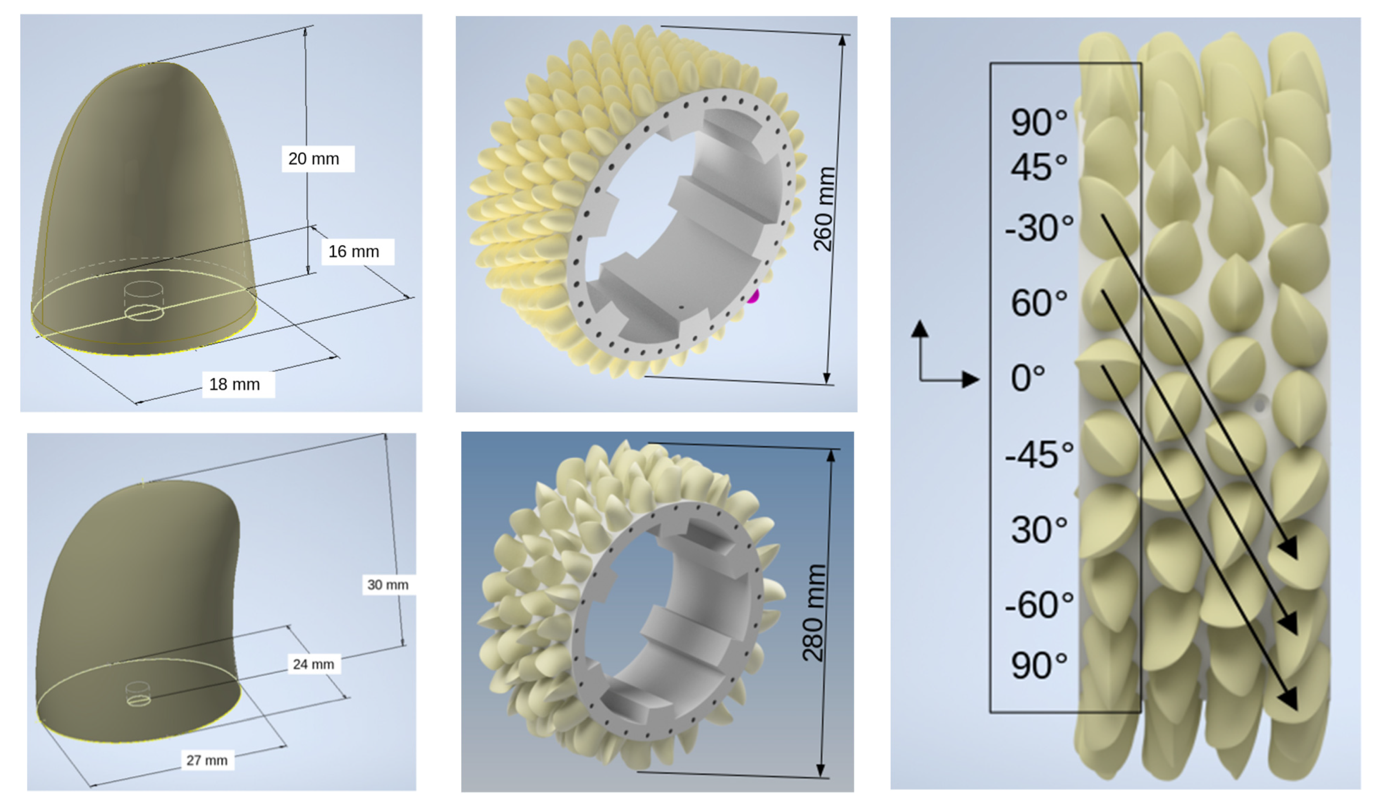
2.1. Realistic Shape of Colonization by Mussels
- − to analyze the effect of a realistic roughness on the loading and to compare with other tests in the literature,
- − to highlight whether the realistic size of mussels significantly impacts the loading.
2.2. Realistic Hydrodynamic Configurations
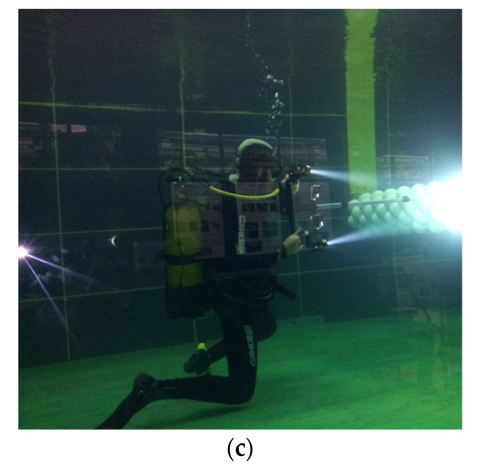
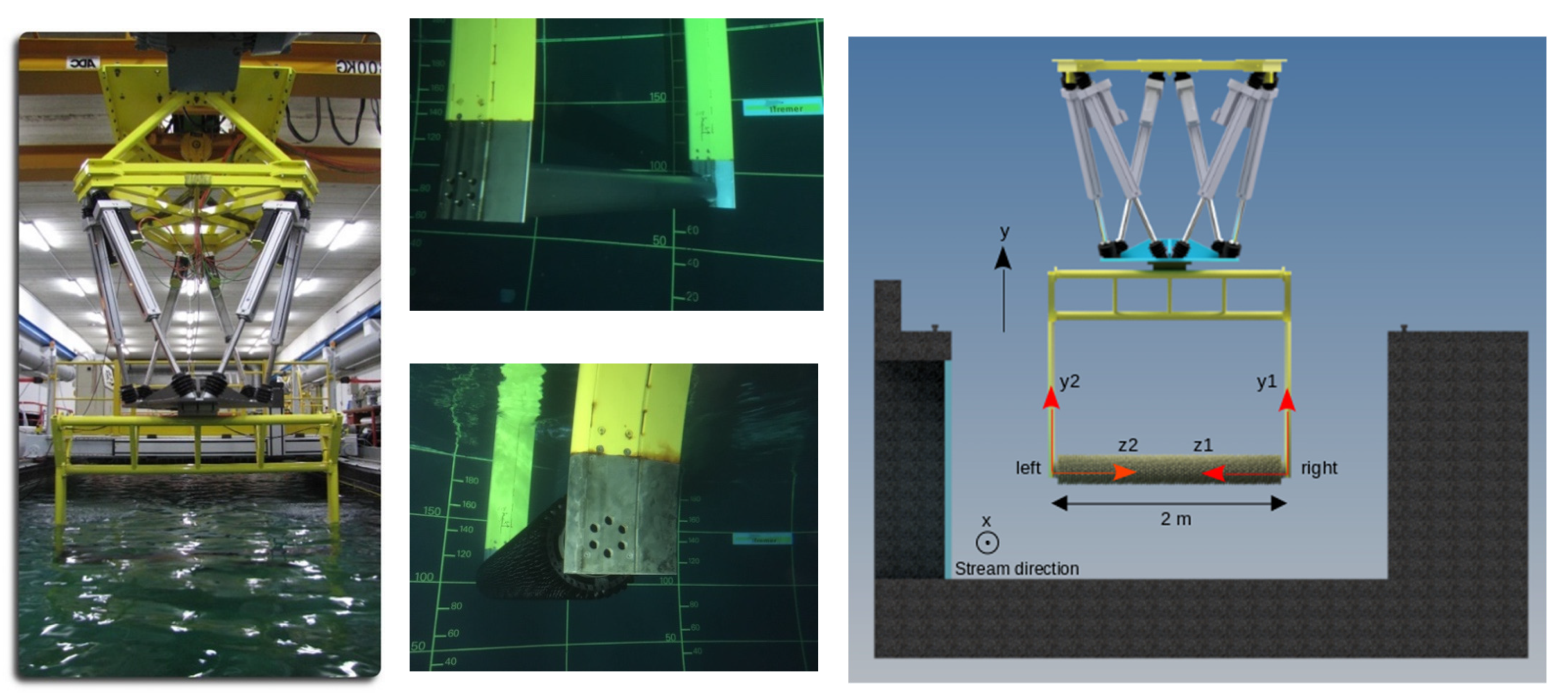
3. Experimental Setup
3.1. Ifremer Flume Tank, Assembly and Instrumentation
3.2. Post-Processing of Results
- − CD for the drag coefficient in steady flow (also written CDS in standards)
- − Cd for the drag coefficient in oscillating motion (also written CD in standards)
- − Cm for the inertia coefficient in oscillating motion (also written CM in standards).
- − Current only
- − Oscillating motion
- − Current and oscillating motion
4. Results and Discussion
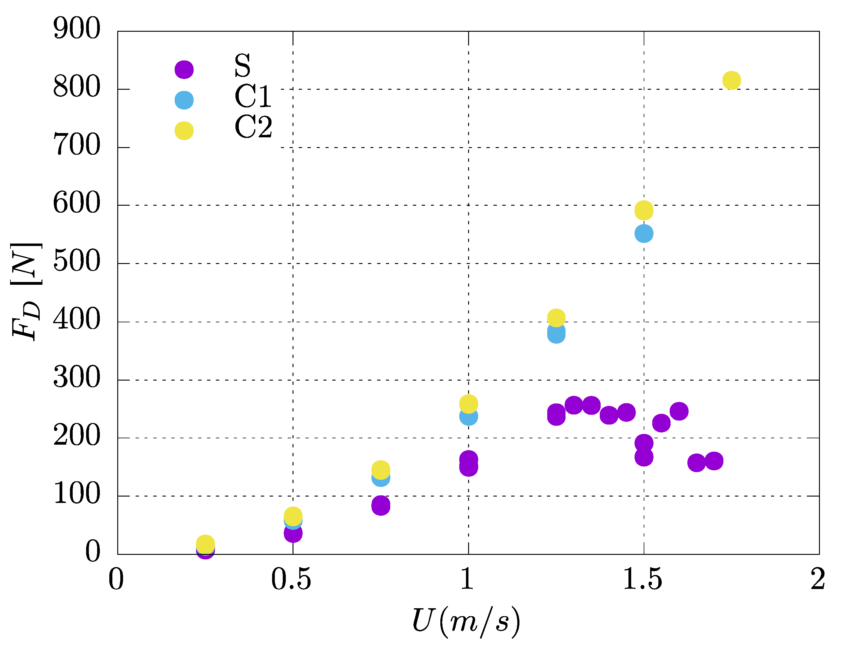
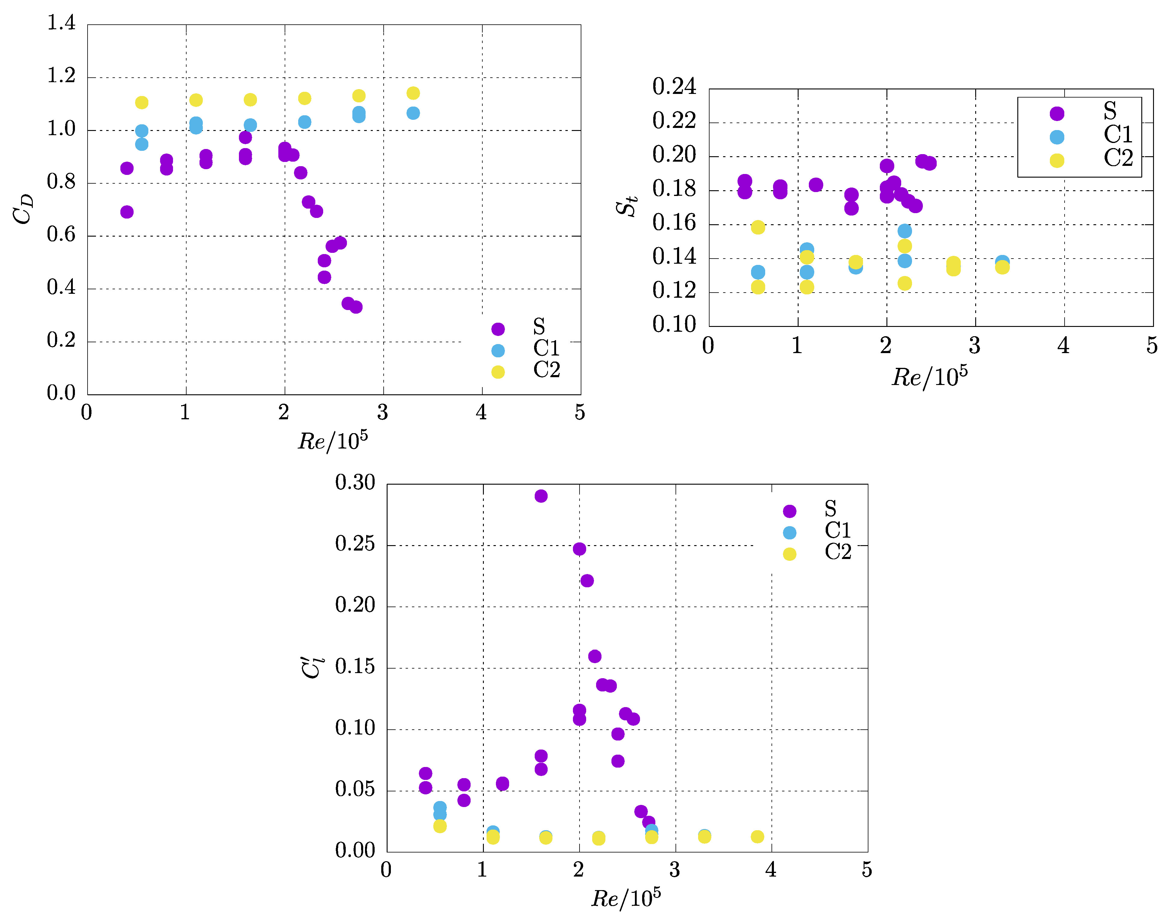
4.1. Current Only Tests
- − Areal density for C1 = 2969 specimens/m2.
- − Areal density for C2 = 1374.5 specimens/m2.
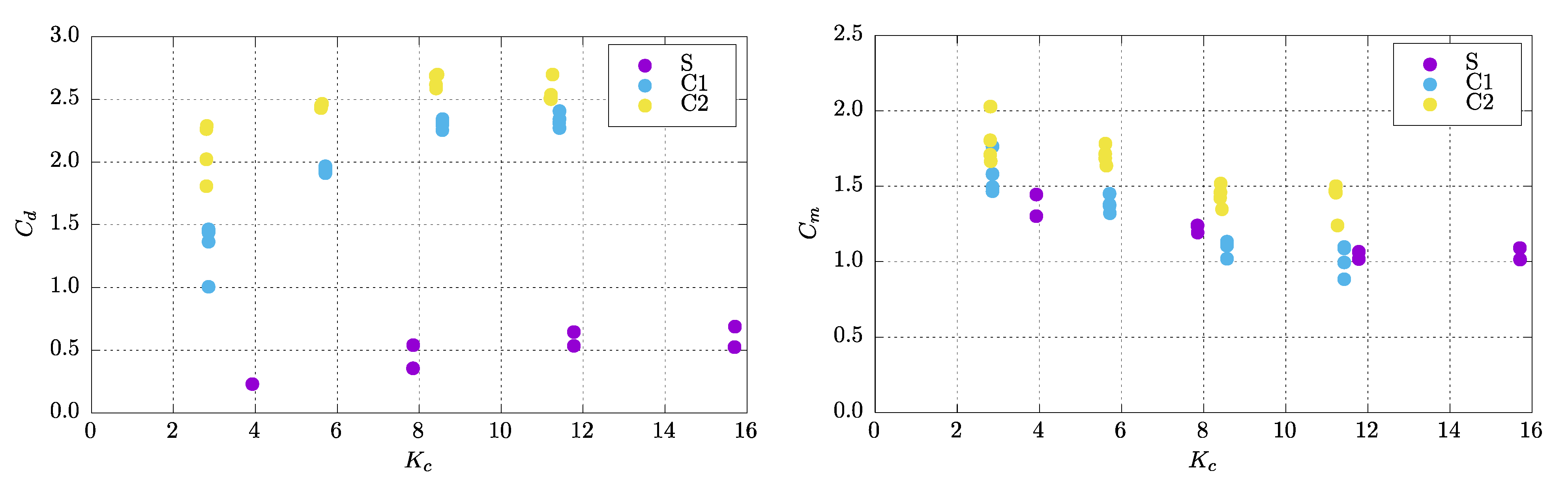
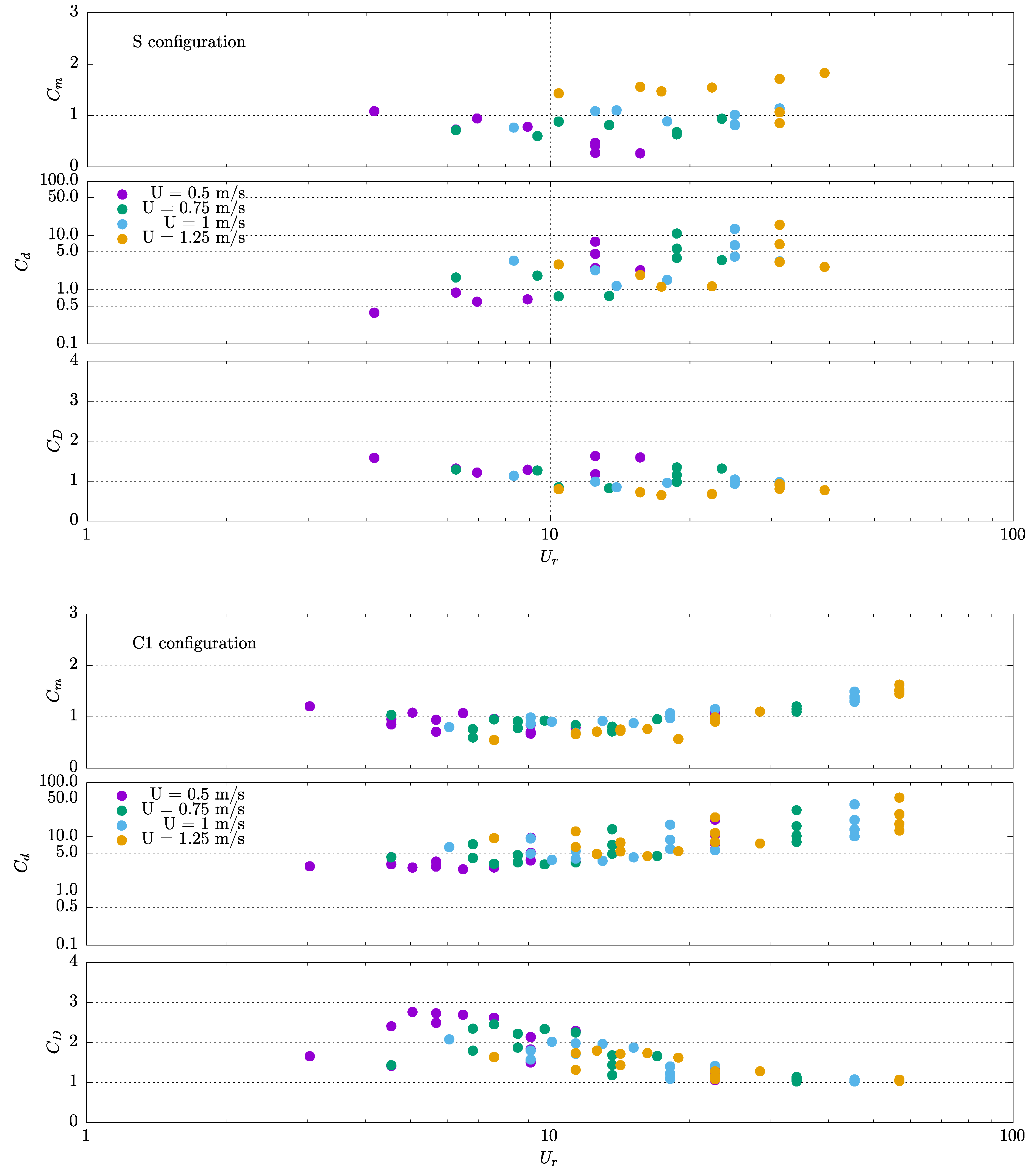
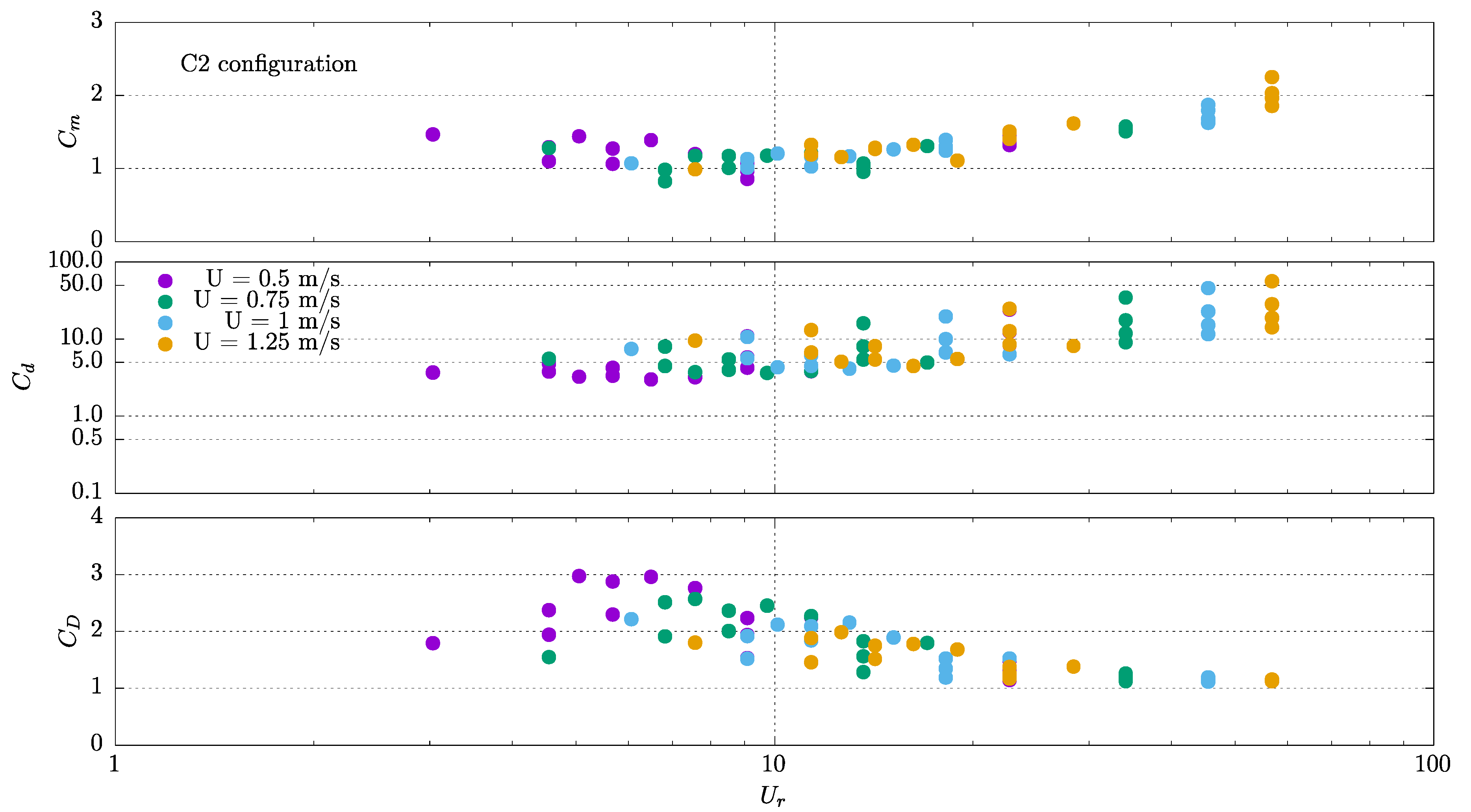
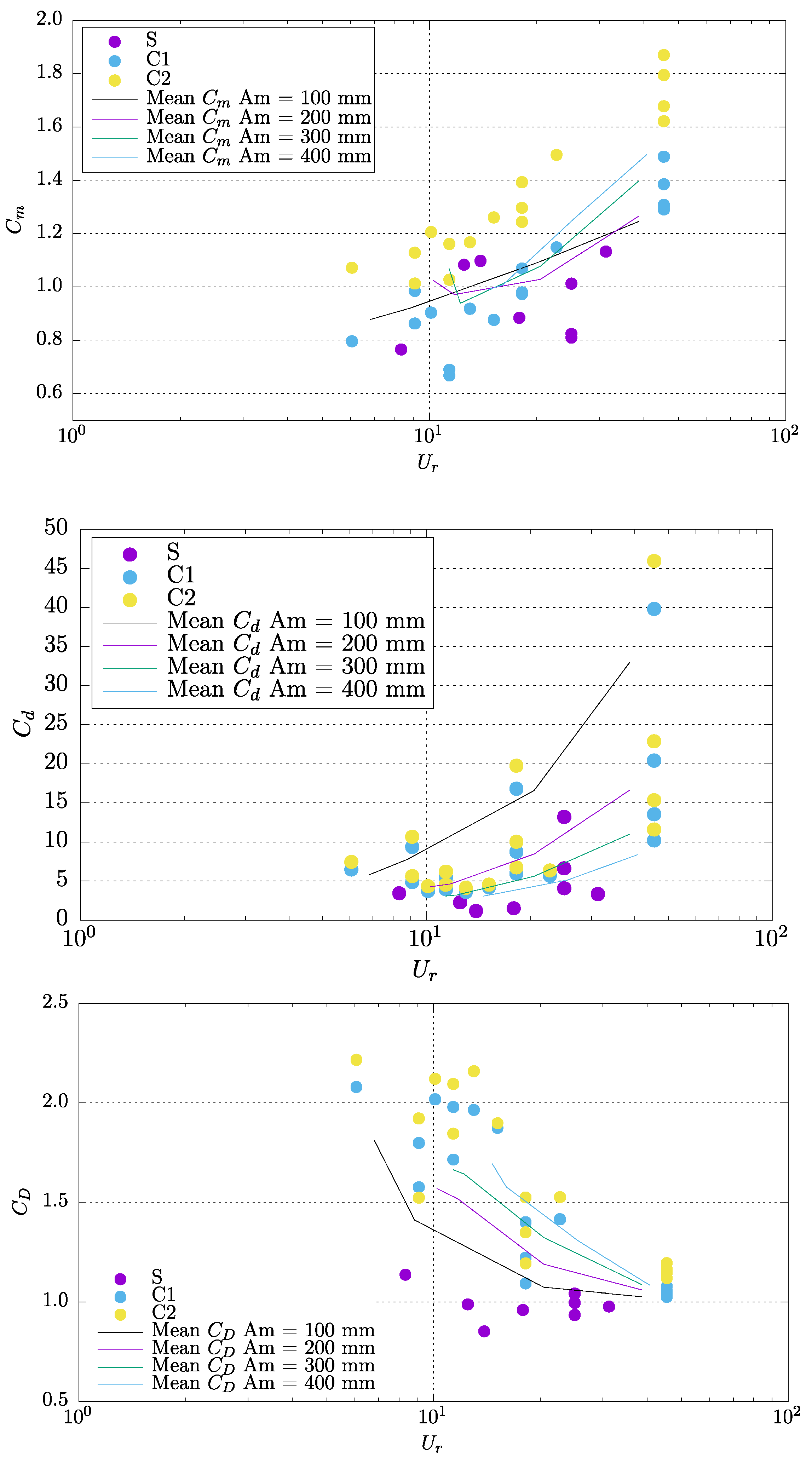
4.2. Oscillating Motions
4.3. Current and Oscillating Motions
5. Discussion and Conclusions
Author Contributions
Funding
Institutional Review Board Statement
Informed Consent Statement
Data Availability Statement
Conflicts of Interest
References
- IEA. World Energy Outlook 2019; Energy Outlook Report; IEA: Paris, France, 2019; Available online: https://www.iea.org/reports/world-energy-outlook-2019 (accessed on 1 November 2019).
- Spraul, C.; Arnal, V.; Cartraud, P.; Berhault, C. Parameter Calibration in Dynamic Simulations of Power Cables in Shallow Water to Improve Fatigue Damage Estimation. In OMAE International Conference; The American Society of Mechanical Engineers: Trondheim, Norway, 2017. [Google Scholar] [CrossRef]
- Decurey, B.; Schoefs, F.; Barillé, A.L.; Soulard, T. Model of Bio-Colonisation on Mooring Lines: Updating Strategy based on a Static Qualifying Sea State for Floating Wind Turbine. J. Mar. Sci. Eng. 2020, 8, 108. [Google Scholar] [CrossRef]
- Ma, K.T.; Duggal, A.; Smedley, P.; L’hostis, D.; Shu, H. A Historical Review on Integrity Issues of Permanent Mooring Systems. In Proceedings of the Offshore Technology Conference, Houston, TX, USA, 6 May 2013. [Google Scholar] [CrossRef]
- Fontaine, E.; Kilner, A.; Carra, C.; Washington, D.; Ma, K.T.; Phadke, A.; Laskowski, D.; Kusinski, G. Industry Survey of Past Failures, Pre-emptive Replacements and Reported Degradations for Mooring Systems of Floating Production Units. In Proceedings of the Offshore Technology Conference, Houston, TX, USA, 5 May 2014. [Google Scholar] [CrossRef]
- James, R.; Weng, W.Y.; Spradbery, C.; Jones, J.; Matha, D.; Mitzlaff, A.; Ahilan, R.V.; Frampton, M.; Lopes, M. Floating Wind Joint Industry Project—Phase I Summary Report. Carbon Trust Tech. Rep. 2018, 19, 2–20. [Google Scholar]
- Braithwaite, R.A. McEvoy, L.A. Marine biofouling on fish farms and its remediation. Adv. Mar. Biol. 2005, 47, 215–252. [Google Scholar] [CrossRef]
- Morison, J.R.; Johnson, J.W.; Schaaf, S.A. The Force Exerted by Surface Waves on Piles. J. Pet. Technol. 1950, 2, 149–154. [Google Scholar] [CrossRef]
- Heaf, N.J. The Effect of Marine Growth on The Performance of Fixed Offshore Platforms in the North Sea. In Proceedings of the Offshore Technology Conference, Houston, TX, USA, 30 April 1979; p. 14. [Google Scholar] [CrossRef]
- Jusoh, I.; Wolfram, J. Effects of marine growth and hydrodynamic loading on offshore structures. J. Mek. 1996, 1, 77–98. [Google Scholar]
- Spraul, C.; Pham, H.D. Effect of Marine Growth on Floating Wind Turbines Mooring Lines Responses. In Proceedings of the 23ème Congrès Français de Mécanique, Lille, France, 1 September 2017. [Google Scholar]
- Schoefs, F. Sensitivity approach for modelling the environmental loading of marine structures through a matrix response surface. Reliab. Eng. Syst. Saf. 2008, 93, 1004–1017. [Google Scholar] [CrossRef][Green Version]
- Schoefs, F.; Boukinda, M.L. Sensitivity Approach for Modeling Stochastic Field of Keulegan–Carpenter and Reynolds Numbers Through a Matrix Response Surface. J. Offshore Mech. Arct. Eng. 2010, 132, 011602. [Google Scholar] [CrossRef]
- Wolfram, J.; Jusoh, I.; Sell, D. Uncertainty in the Estimation of Fluid Loading Due to the Effects of Marine Growth. In Proceedings of the 12th International Conference on Offshore Mechanical and Arctic Engineering, Glasgow, UK, 20–24 June 1993; Volume 2, pp. 219–228. [Google Scholar]
- Zeinoddini, M.; Bakhtiari, A.; Schoefs, F.; Zandi, A.P. Towards an Understanding of the Marine Fouling Effects on VIV of Circular Cylinders: Partial Coverage Issue. Biofouling 2017, 33, 268–280. [Google Scholar] [CrossRef]
- Sarpkaya, T. On the Effect of Roughness on Cylinders. J. Offshore Mech. Arct. Eng. 1990, 112, 334. [Google Scholar] [CrossRef]
- Ameryoun, H.; Schoefs, F.; Barillé, L.; Thomas, Y. Stochastic Modeling of Forces on Jacket-Type Offshore Structures Colonized by Marine Growth. J. Mar. Sci. Eng. 2019, 7, 158. [Google Scholar] [CrossRef]
- Theophanatos, A. Marine Growth and the Hydrodynamic Loading of Offshore Structures. Ph.D. Thesis, University of Strathclyde, Glasgow, UK, 1988. Available online: https://ethos.bl.uk/OrderDetails.do?uin=uk.bl.ethos.382439 (accessed on 1 February 1988).
- API RP 2A WSD. Recommended Practice for Planning, Designing, and Constructing Fixed Offshore Platforms; The American Petroleum Institute: Washington, DC, USA, 2005; Volume 2. [Google Scholar]
- DNV. Recommended Practice DNV-RP-C205: Environmental Conditions and Environmental Loads; Det Norske Veritas: Bærum, Norway, 2010. [Google Scholar]
- Page, H.M.; Hubbard, D.M. Temporal and spatial patterns of growth in mussels Mytilus edulis on an offshore platform: Relationships to water temperature and food availability. J. Exp. Mar. Biol. Ecol. 1987, 111, 159–179. [Google Scholar] [CrossRef]
- Parks, T.; Sell, D.; Picken, G. Marine Growth Assessment of Alwyn North A in 1994; Technical Report 820; Auris Environmental LTD: Coventry, UK, 1995. [Google Scholar]
- Boukinda Mbadinga, M.L.; Quiniou Ramus, V.; Schoefs, F. Marine Growth Colonization Process in Guinea Gulf: Data Analysis. J. Offshore Mech. Arctic Eng. 2007, 129, 97–106. [Google Scholar] [CrossRef]
- Handå, A.; Alver, M.; Edvardsen, C.V.; Halstensen, S.; Olsen, A.J.; Øie, G.; Reinertsen, H. Growth of farmed blue mussels (Mytilus edulis L.) in a Norwegian coastal area: Comparison of food proxies by DEB modeling. J. Sea Res. 2011, 66, 297–307. [Google Scholar] [CrossRef]
- O’Byrne, M.; Schoefs, F.; Pakrashi, V.; Ghosh, B. An underwater lighting and turbidity image repository for analysing the performance of image based non-destructive techniques. Struct. Infrastruct. Eng. Maint. Manag. Life Cycle Des. Perform. 2018, 14, 104–123. [Google Scholar] [CrossRef]
- O’Byrne, M.; Schoefs, F.; Pakrashi, V.; Ghosh, B. A Stereo-Matching Technique for Recovering 3D Information from Underwater Inspection Imagery. Comput. Aided Civ. Infrastruct. Eng. 2018, 33, 193–208. [Google Scholar] [CrossRef]
- O’Byrne, M.; Pakrashi, V.; Schoefs, F.; Ghosh, B. Semantic Segmentation of Underwater Imagery Using Deep Networks. J. Mar. Sci. Eng. Sect. Ocean Eng. 2018, 6, 93. [Google Scholar] [CrossRef]
- O’Byrne, M.; Pakrashi, V.; Schoefs, F.; Ghosh, B. Applications of Virtual Data in Subsea Inspections. J. Mar. Sci. Eng. Sect. Ocean Eng. 2020, 8, 328. [Google Scholar] [CrossRef]
- Picken, G.B. Review of marine fouling organisms in the North Sea on offshore structures. Discussion Forum and Exhibition on Offshore Engineering with Elastomers. Plast. Rubber Inst. 1985, 5, 1–5. [Google Scholar]
- Schoefs, F.; O’Byrne, M.; Pakrashi, V.; Ghosh, B.; Oumouni, M.; Soulard, T.; Reynaud, M. Feature-Driven Modelling and Non-Destructive Assessment of Hard Marine Growth Roughness from Underwater Image Processing. J. Mar. Sci. Eng. 2021, accepted. [Google Scholar]
- Achenbach, E.; Heinecke, E. On vortex shedding from smooth and rough cylinders in the range of Reynolds numbers 6e3 to 5e6. J. Fluid Mech. 1981, 109, 239–251. [Google Scholar] [CrossRef]
- Gaurier, B.; Germain, G.; Facq, J.; Baudet, L.; Birades, M.; Schoefs, F. Marine growth effects on the hydrodynamical behaviour of circular structures. In Proceedings of the 14th Journées de l’Hydrodynamique, Val de Reuil, France, 18–20 November 2014. [Google Scholar]
- Sarpkaya, T. Moirison’s Equation and the Wave Forces on Offshore Structures; Technical Report; Naval Civil Engineering Laboratory: Carmel, CA, USA, 1981. [Google Scholar]
- Marty, A.; Germain, G.; Facq, J.V.; Gaurier, B.; Bacchetti, T. Experimental investigation of the marine growth effect on the hydrodynamical behavior of a submarine cable under current and wave conditions. In Proceedings of the JH2020-17èmes Journées de l’Hydrodynamique, Cherbourg, France, 4–26 November 2020. [Google Scholar] [CrossRef]
- Marty, A.; Berhault, C.; Damblans, G.; Facq, J.-V.; Gaurier, B.; Germain, G.; Soulard, T.; Schoefs, F. Experimental study of marine growth effect on the hydrod-ynamical behaviour of a submarine cable. Appl. Ocean. Res. 2021. in Press. [Google Scholar]
- Schlichting, H. Boundary Layer Theory; McGraw-Hill: New York, NY, USA, 1979. [Google Scholar]
- Verley, R.L.P. Oscillations of Cylinders in Waves and Currents. Ph.D. Thesis, Loughborough University of Technology, Loughborough, UK, 1980. [Google Scholar]
- Molin, B. Hydrodynamique des Structures Offshore; Technip Editions: Paris, France, 2002. [Google Scholar]
- Melbourne, W.H.; Blackburn, H.M. The effect of free-stream turbulence on sectional lift forces on a circular cylinder. J. Fluid. Mech. 1996, 11, 267–292. [Google Scholar]
- Sarpkaya, T. In-Line and Transverse Forces on Smooth and Sand Roughened Circular Cylinders in Oscillating Flow at High Reynolds Numbers; Technical Report No. NPS-69SL; Naval Postgraduate School: Monterey CA, USA, 1976. [Google Scholar]
- Rodenbusch, G.; Gutierrez, C.A. Forces on Cylinders in Two Dimensional Flow; Technical Report No. BRC 123-83; Bellaire Research Center: Houston, TX, USA, 1983; Volume 1. [Google Scholar]
- Nath, J.H. Heavily roughened horizontal cylinders in waves. Proc. Conf. Behav. Offshore Struct. 1982, 1, 387–407. [Google Scholar]


| N° Position/Angle | 1 | 2 | 3 | 4 | 5 | 6 | 7 | 8 | 9 | 10 | 11 | 12 | 13 | 14 | 15 | 16 |
|---|---|---|---|---|---|---|---|---|---|---|---|---|---|---|---|---|
| X | 8 | 25 | 41 | 58 | 8 | 24 | 43 | 59 | 8 | 26 | 42 | 58 | 8 | 25 | 41 | 58 |
| Y | 59 | 58 | 58 | 59 | 42 | 42 | 42 | 41 | 26 | 25 | 26 | 23 | 9 | 8 | 9 | 8 |
| Inclination of major axis/axis x | +45° | −30° | +30° | −45° | +45° | +45° | +90° | 0° | +45° | +90° | 0° | +90° | 0° | −30° | +30° | +60° |
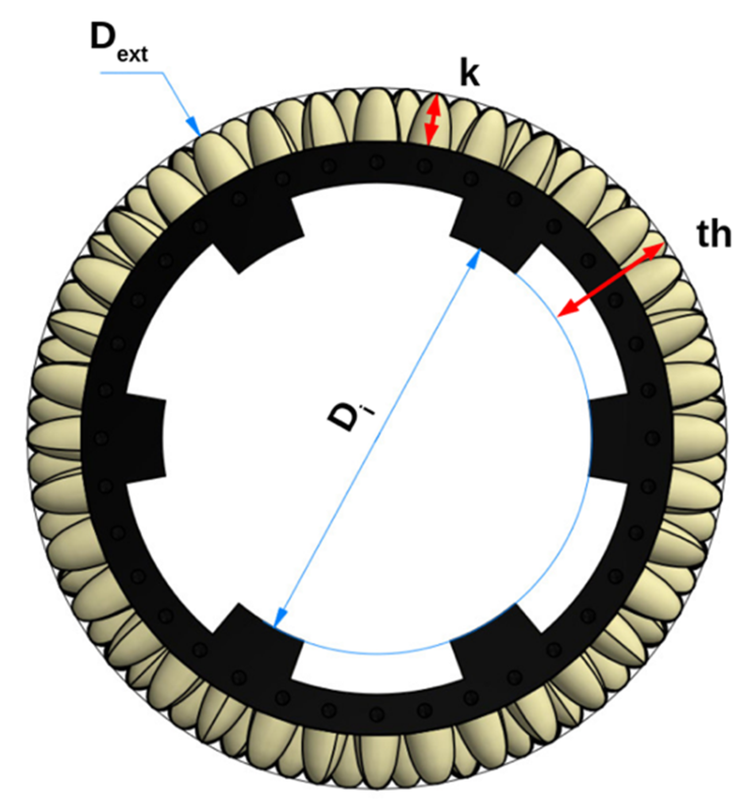
| Configurations | Di [mm] | Dext [mm] | k [mm] | th [mm] | De [mm] | e = k/De | Mass System [daN] | Areal Density for nb. Specimens/m2 |
|---|---|---|---|---|---|---|---|---|
| S | 160 | 160 | 0 | 0 | 160 | 0 | 47 | - |
| C1 | 160 | 260 | 20 | 50 | 220 | 0.091 | 105 | 2969 |
| C2 | 160 | 280 | 30 | 60 | 220 | 0.136 | 110 | 1374.5 |
| Configurations | KC | Ur | Re/105 |
|---|---|---|---|
| S | 3.9–15.7 | 4.1–39.1 | 0.4–2.7 |
| C1 | 2.5–11.4 | 3–56.8 | 0.55–3.8 |
| C2 | 2.5–11.4 | 3–56.8 | 0.55–3.8 |
Publisher’s Note: MDPI stays neutral with regard to jurisdictional claims in published maps and institutional affiliations. |
© 2021 by the authors. Licensee MDPI, Basel, Switzerland. This article is an open access article distributed under the terms and conditions of the Creative Commons Attribution (CC BY) license (https://creativecommons.org/licenses/by/4.0/).
Share and Cite
Marty, A.; Schoefs, F.; Soulard, T.; Berhault, C.; Facq, J.-V.; Gaurier, B.; Germain, G. Effect of Roughness of Mussels on Cylinder Forces from a Realistic Shape Modelling. J. Mar. Sci. Eng. 2021, 9, 598. https://doi.org/10.3390/jmse9060598
Marty A, Schoefs F, Soulard T, Berhault C, Facq J-V, Gaurier B, Germain G. Effect of Roughness of Mussels on Cylinder Forces from a Realistic Shape Modelling. Journal of Marine Science and Engineering. 2021; 9(6):598. https://doi.org/10.3390/jmse9060598
Chicago/Turabian StyleMarty, Antoine, Franck Schoefs, Thomas Soulard, Christian Berhault, Jean-Valery Facq, Benoît Gaurier, and Gregory Germain. 2021. "Effect of Roughness of Mussels on Cylinder Forces from a Realistic Shape Modelling" Journal of Marine Science and Engineering 9, no. 6: 598. https://doi.org/10.3390/jmse9060598
APA StyleMarty, A., Schoefs, F., Soulard, T., Berhault, C., Facq, J.-V., Gaurier, B., & Germain, G. (2021). Effect of Roughness of Mussels on Cylinder Forces from a Realistic Shape Modelling. Journal of Marine Science and Engineering, 9(6), 598. https://doi.org/10.3390/jmse9060598