Cavity Detachment from a Wedge with Rounded Edges and the Surface Tension Effect

Abstract

Cavity flow around a wedge with rounded edges was studied, taking into account the surface tension effect and the Brillouin–Villat criterion of cavity detachment. The liquid compressibility and viscosity were ignored. An analytical solution was obtained in parametric form by applying the integral hodograph method. This method gives the possibility of deriving analytical expressions for complex velocity and for potential, both defined in a parameter plane. An expression for the curvature of the cavity boundary was obtained analytically. By using the dynamic boundary condition on the cavity boundary, an integral equation in the velocity modulus was derived. The particular case of zero surface tension is a special case of the solution. The surface tension effect was computed over a wide range of the Weber number for various degrees of cavitation development. Numerical results are presented for the flow configuration, the drag force coefficient, and the position of cavity detachment. It was found that for each radius of the edges, there exists a critical Weber number, below which the iterative solution process fails to converge, so a steady flow solution cannot be computed. This critical Weber number increases as the radius of the edge decreases. As the edge radius tends to zero, the critical Weber number tends to infinity, or a steady cavity flow cannot be computed at any finite Weber number in the case of sharp wedge edges. This shows some limitations of the model based on the Brillouin–Villat criterion of cavity detachment.

1. Introduction

Surface tension arises at an air–liquid interface as a result of a reversible isothermokinetic process on a free boundary. According to the Young–Laplace equation, surface tension results in a pressure jump, which is governed by the curvature of the cavity boundary. The dynamic boundary condition in the model of the ideal fluid (Bernoulli equation) includes this jump; therefore, the velocity modulus on the cavity boundary, the pressure on the liquid side of the interface, and the curvature of the interface are related to one another. Cavity detachment for smooth-shaped bodies is determined by the Brillouin–Villat criterion [1,2], which states that the curvature of the cavity boundary should be equal to the curvature of the body at the point of detachment. This criterion comes from geometrical restrictions on the cavity curve and, therefore, it should be valid for flows both with and without surface tension. As the surface tension tends to zero, the solution of the problem gradually approaches its limiting case without surface tension, as shown in [3], for cavity flow past a circular cylinder.

Cavity detachments for bodies whose shapes form corner trailing edges are different, and it is not fully understood yet when the surface tension is nonzero. Although the position of cavity detachment is predetermined at the edge, the curvature of the cavity boundary is infinite for the case of zero surface tension [4,5]. Even small surface tension might result in an infinite negative pressure at the cavity detachment point. The same infinite negative pressure occurs for flow around a corner without flow detachment. Therefore, flow detachment may not occur at all.

Attempts to take into account surface tension in problems of cavity flows were done in [6,7,8,9]. The case of small surface tension values was considered in [8] using the method of matched asymptotic expansions. For this case, the curvature of the cavity boundary equals the curvature of the plate at the point of detachment. Such a formulation of the problem leads to waves on the free surface. It was shown in [9] that these waves have no physical basis since they require an energy input from infinity. In [6,7], it is assumed that at the flow detachment point, the tangent to the flow boundary is a discontinuous function. According to the theory of jets of an ideal liquid [4,5], this assumption leads to zero velocity at the point, while the curvature of the cavity boundary remains undetermined. Alternative models of cavity detachment were proposed in the works [10,11]. These models account for the physical properties of the liquid/structure interaction [12,13]. The work [10] considers cavity detachment as bubbles growing within the boundary layer starting from the stagnation point; the coalition and merging of the bubbles form a cavity. The work [11] considers adhesion between the liquid and the material of the body, which determines the contact angle between the body and the free surface. However, these models are not used widely in practice since further experimental validation of these models is required.

The surface tension force becomes dominant on the scale of mechanical elements far below millimeters, which is the typical size of microelectromechanical systems (MEMS) and microfluidic systems [14,15]. The study of cavitation phenomena in such systems is of interest when developing micropumps, microvalves, microcoolers, etc., which are fabricated with a micro-orifice of a smaller diameter than the main microchannel. Cavitation in MEMS appears in the same way as cavitation in macroscale devices, when the local pressure drops below the vapor pressure. However, on microscale, the surface tension force dominates other forces and may affect flow characteristics, which may be treated as a scale effect [16,17].

In this paper, we consider classical two-dimensional potential free surface flow around a wedge with rounded edges and apply the Brillouin–Villat criterion to determine the cavity detachment for the case of nonzero surface tension. A sharp trailing edge is considered as the limiting case of a rounded edge when the radius of the edge tends to zero. An analytical solution to the problem is obtained using the integral hodograph method [18]. The complex velocity and the derivative of the complex potential are derived analytically in a parameter plane. A function mapping the parameter plane onto the physical plane is also obtained. The method is based on the integral formula [19], which gives a solution of a mixed boundary-value problem for a complex function (here, the complex velocity) defined in the first quadrant. The derivative of the complex potential is obtained by using Chaplygin’s singular point method [5,20].

The complex velocity includes the slope to the body and the velocity modulus along the cavity boundary, which are determined from a system of integral equations derived by using the dynamic and the kinematic boundary conditions. By using an analytical expression for the curvature of the free boundary, it is possible to directly apply the Brillouin–Villat condition and obtain an equation to determine the point of cavity detachment.

The results are presented over a wide range of Weber numbers and the radius of the wedge edges. It is shown that the effect of surface tension becomes more pronounced as the Weber number or the radius of the edge decrease. The surface tension results in some reduction of the cavity length and the drag force coefficient and delays cavity detachment. The point of detachment moves downward, increasing the wetted part of the rounded edge. It is found that, for each edge radius, there exists a critical Weber number below which a solution cannot be obtained due to the iteration process failing to converge. This critical Weber number increases as the radius of the edge decreases. As the edge radius tends to zero, the Weber number tends to infinity, or a steady cavity flow cannot be computed for any finite Weber number in the case of a sharp wedge edge. This shows some limitation of the model based only on the Brillouin–Villat criterion of detachment.

2. Complex Potential of the Flow

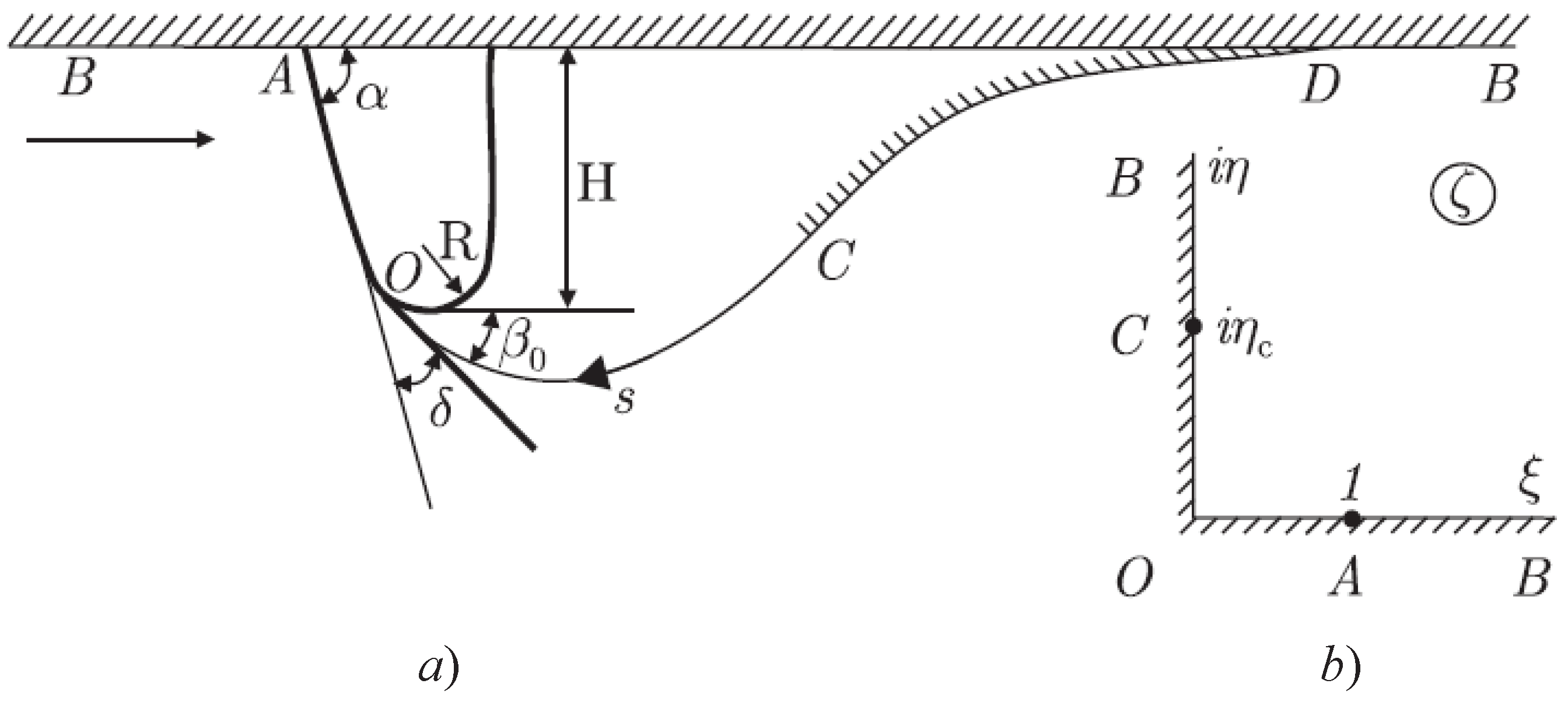
We consider cavity flow past a wedge of width $2H$ with rounded edges of radius R sketched in Figure 1a. The wedge angle $\alpha$ lies in the range $0<\alpha <\pi$. For $\alpha ={90}^{\circ }$, the wedge becomes a flat plate. We introduce Cartesian coordinates $xy$. The origin is located at point O. The liquid is inviscid and incompressible. The flow is symmetric about the $x$-axis, so we consider only half of the flow region. An assumption as to the cavity closure is necessary due to the Brillouin paradox at the point where the upper and the lower cavity boundaries are merged [4]. We introduce an implicit model of cavity closure according to which, along the streamline $OCDB$, the velocity modulus changes in such a manner that the portion $OC$ corresponds to the cavity boundary, and on the portion $CD$ the velocity modulus changes from the value $V_0$ at the end of the cavity (point C) to the value U at point D. The velocity U is the velocity at infinity. Along the contour $DB$, the velocity remains constant and equals U. As $s\to \infty$, the $y$-coordinate of the closing line $DB$ tends to zero. Such a cavity closure model mimics a turbulent wake in real cavity flows [21,22].

The pressure jump across the cavity boundary is determined by the Laplace–Young formula

$$p-p_c=\tau \mathsf{{\rm Y}},$$

(1)

where $\tau$ is the coefficient of surface tension, $p_c$ is the pressure in the cavity, and $\mathsf{{\rm Y}}$ is the curvature. The pressure in the cavity may be equal to the vapor pressure, $p_c=p_v$, or be higher for gaseous liquids.

We choose H and U as the characteristic length and velocity, respectively. From the equation

$$\frac{V^2}{2}+\frac{p}{\rho }=\frac{U^2}{2}+\frac{p_{\infty }}{\rho }$$

(2)

and Equation (1) the velocity modulus on the cavity boundary is obtained

$$v=\frac{V}{U}=\sqrt{1+\sigma -\frac{2\chi }{We}},$$

(3)

where $\chi =\mathsf{{\rm Y}}H$. Here, $We$ is the Weber number that characterizes the ratio of the inertia force to the surface tension force, and $\sigma$ is the cavitation number indicating the degree of cavitation development.

$$\sigma =\frac{p_{\infty }-p_c}{1/2\rho U^2},We=\frac{\rho U^{2}H}{\tau },$$

(4)

where $\rho$ is the density of the liquid, and $p_{\infty }$ is the pressure at infinity.

We can introduce a complex potential, $w\left(z\right)=\varphi (x,y)+i\psi (x,y)$, where $\varphi (x,y)$ and $\psi (x,y)$ are the harmonic conjugate function of the potential and the stream function, respectively. The determination of the function $w\left(z\right)$ is a challenging problem. Instead, Michell [23] and Joukovskii [24] introduced an auxiliary $\zeta$-plane and determined the complex conjugate velocity, $dw/dz$, and the derivative of the complex potential, $dw/d\zeta$, as functions of the parameter variable $\zeta$. If these functions are known, then the solution of the problem is obtained in parametric form:

$$w\left(\zeta \right)=w_0+{\int }_0^{\zeta }\frac{dw}{d{\zeta }^{\prime }}d{\zeta }^{\prime },z\left(\zeta \right)=z_0+{\int }_0^{\zeta }\frac{dw}{d{\zeta }^{\prime }}/\frac{dw}{dz}d{\zeta }^{\prime },$$

(5)

where $w_0$ is the value of the complex potential at point O, and $z_0$ is the coordinate of point O.

We choose the first quadrant of the $\zeta$-plane in Figure 1b as the region corresponding to the liquid region in the physical plane (Figure 1a). According to the conformal mapping theorem, we can chose the position of three points. They are points O ($\zeta =0$), A ($\zeta =1$), and B ($\zeta =\infty$), as shown in Figure 1b. The interval $0<\xi <1$ corresponds to the wetted part of the wedge, and the interval $1<\xi <\infty$ corresponds to the symmetry line $AB$. The imaginary $\eta$-axis corresponds to the boundary $OCDB$, which includes the cavity contour $OC$ ($0<\eta <{\eta }_c$) and the closure contour $CB$ (${\eta }_c<\eta <\infty$). The position of point C ($\zeta =i{\eta }_c$) has to be determined from the solution of the problem and physical considerations. In order to determine these functions, we assume that the velocity modulus v and the tangent to the wetted part of the body $\beta$ are known functions of the variables $\eta$ and $\xi$, respectively.

2.1. Expressions for the Complex Velocity and for the Derivative of the Complex Potential

The body is considered to be fixed; therefore, the velocity direction and the slope of the body coincide. Besides, at this stage we assume that the velocity magnitude on the free surface is a known function of the parameter variable, $v\left(\eta \right)$. Then the boundary-value problem for the complex velocity in the first quadrant of the parameter plane can be written as follows

$$\chi \left(\xi \right)=arg\left(\frac{dw}{dz}\right)=\left\{\begin{array}{c}-{\beta }_b\left(\xi \right),0\le \xi \le 1,\hfill \\ 0,1\le \xi <\infty .\hfill \end{array}\right.$$

(6)

$$v\left(\eta \right)={\left|\frac{dw}{dz}\right|}_{\zeta =i\eta },0\le \eta <\infty .$$

(7)

Here, ${\beta }_b{\left(\xi \right)}_{\xi =0}={\beta }_0$ at point O, and ${\beta }_b\left(\xi \right)=-\alpha$ as $\xi \to 1$. Equation (6) satisfies the conditions: $\chi \left(\xi \right)=0$ along the interval $AB$ on the symmetry line and $\chi \left(\xi \right)=-{\beta }_b\left(\xi \right)$ along the body. The argument of the complex velocity exhibits a jump $\mathsf{\Delta }=\alpha$ at point A when we move along the boundary in the physical plane from point O to point B. This boundary-value problem can be solved by applying the following integral formula [19]:

$$\frac{dw}{dz}=v_{\infty }exp\left[\frac{1}{\pi }\underset{0}{\overset{\infty }{\int }}\frac{d\chi }{d\xi }ln\left(\frac{\zeta +\xi }{\zeta -\xi }\right)d\xi -\frac{i}{\pi }\underset{0}{\overset{\infty }{\int }}\frac{dlnv}{d\eta }ln\left(\frac{\zeta -i\eta }{\zeta +i\eta }\right)d\eta +i{\chi }_{\infty }\right],$$

(8)

where $v_{\infty }=v{\left(\eta \right)}_{\eta \to \infty }$ and ${\chi }_{\infty }=\chi {\left(\xi \right)}_{\xi \to \infty }$. Substituting Equations (6) and (7) into (8) and evaluating the first integral over the step change at the point $\zeta =1$, we obtain

$$\begin{array}{c}\hfill \frac{dw}{dz}={\left(\frac{\zeta -1}{\zeta +1}\right)}^{\frac{\alpha }{\pi }}exp\left[\frac{1}{\pi }\underset{0}{\overset{1}{\int }}\frac{d{\beta }_b}{d\xi }ln\left(\frac{\zeta -\xi }{\zeta +\xi }\right)d\xi -\frac{i}{\pi }\underset{0}{\overset{\infty }{\int }}\frac{dlnv}{d\eta }ln\left(\frac{\zeta -i\eta }{\zeta +i\eta }\right)d\eta \right].\end{array}$$

(9)

Here, we used $v_{\infty }=1$, which follows from the definition. It can be easily verified that for $\zeta =\xi$ the argument of the right-hand side of (9) is the function $-{\beta }_b\left(\xi \right)$, while for $\zeta =i\eta$ the modulus of (9) is the function $v\left(\eta \right)$, i.e., the boundary conditions (6) and (7) are satisfied. It can also be seen that the complex velocity function has zeros of order $\alpha /\pi$, which correspond to flow around a corner of angle $\pi -\alpha$ at point A.

The velocity is tangent to the boundary for steady flows and, therefore, $\Im \left(w\right)=0$ both along the body and along the cavity boundary. The real part of the complex potential increases from $-\infty$ at point B to $+\infty$ at point $B^{\prime }$. Thus, the region of the complex potential is a half-plane. The first quadrant and the half-plane of the $w$-plane are related as $w=K{\zeta }^2+w_0$ where K is a positive real number. Then one can obtain

$$\frac{dw}{d\zeta }=K\zeta .$$

(10)

The derivative of the mapping function is obtained by dividing (10) by (9)

$$\begin{array}{c}\hfill \frac{dz}{d\zeta }=K\zeta {\left(\frac{\zeta +1}{\zeta -1}\right)}^{\frac{\alpha }{\pi }}exp\left[-\frac{1}{\pi }\underset{0}{\overset{1}{\int }}\frac{d{\beta }_b}{d\xi }ln\left(\frac{\zeta -\xi }{\zeta +\xi }\right)d\xi +\frac{i}{\pi }\underset{0}{\overset{\infty }{\int }}\frac{dlnv}{d\eta }ln\left(\frac{\zeta -i\eta }{\zeta +i\eta }\right)d\eta \right].\end{array}$$

(11)

The integration of this equation yields the mapping function $z=z\left(\zeta \right)$ relating the parameter and the physical planes. Equations (9) and (10) include the parameter K, and the functions $v\left(\eta \right)$ and ${\beta }_b\left(\xi \right)$, which are determined from the boundary conditions and from physical considerations.

The arc length coordinates along the body, $s_b\left(\xi \right)$, and along the cavity boundary, $s\left(\eta \right)$, are obtained as follows:

$$s_b\left(\xi \right)={\int }_0^{\xi }\frac{d{s}_b}{d\xi }d\xi ,s\left(\eta \right)=-{\int }_0^{\eta }{\left|\frac{dz}{d\zeta }\right|}_{\zeta ={\eta }^{\prime }}d{\eta }^{\prime }=-K{\int }_0^{\eta }\frac{{\eta }^{\prime }}{v\left({\eta }^{\prime }\right)}d{\eta }^{\prime },$$

(12)

where

$$\frac{d{s}_b}{d\xi }={\left|\frac{dz}{d\zeta }\right|}_{\zeta =\xi }=K\xi {\left(\frac{\xi +1}{1-\xi }\right)}^{\alpha /\pi }exp\left(-\frac{1}{\pi }\underset{0}{\overset{1}{\int }}\frac{d{\beta }_b}{d{\xi }^{\prime }}ln\left|\frac{\xi -{\xi }^{\prime }}{\xi +{\xi }^{\prime }}\right|d{\xi }^{\prime }+\frac{1}{\pi }\underset{0}{\overset{\infty }{\int }}\frac{dlnv}{d\eta }2{tan}^{-1}\frac{\eta }{\xi }d\eta \right)$$

(13)

The real factor K is determined from the condition for the length of the wetted part of the wedge, including the trailing edge $S_w$. By substituting Equation (13) into (12), we obtain

$$S_w=K{\int }_0^1{\xi \left(\frac{\xi +1}{1-\xi }\right)}^{\alpha /\pi }exp\left(-\frac{1}{\pi }\underset{0}{\overset{1}{\int }}\frac{d{\beta }_b}{d{\xi }^{\prime }}ln\left|\frac{\xi -{\xi }^{\prime }}{\xi +{\xi }^{\prime }}\right|d{\xi }^{\prime }+\frac{1}{\pi }\underset{0}{\overset{\infty }{\int }}\frac{dlnv}{d\eta }2{tan}^{-1}\frac{\eta }{\xi }d\eta \right)d\xi$$

(14)

2.2. Cavity Closure Model

A solution of the problem of cavity flow around a body is not unique in the framework of the model of ideal liquid due to a paradox that arises at the point of cavity closure. On the one hand, the velocity at this point must be equal to the velocity on the cavity boundary since this point belongs to it. On the other hand, the velocity at this point should be equal to zero since the upper and the lower contours of the cavity merge into one streamline. This is known as the Brillouin paradox [4].

Various assumptions as to the flow in the cavity closure region were proposed by Roshko, Riabouchinsky, Efros, in the re-entrant jet model, Tulin, etc., to resolve this paradox. They are now well known as classical models of cavity flows [5]. These models give similar results for developed cavity flows, for which the size of the cavity is larger than the size of the body. However, when the cavity size is smaller, the cavity contour ends on the body surface (partial cavitation), and the assumptions made may affect the results [10,25].

An implicit cavity closure model modeling effects of the liquid viscosity in the cavity closure region was proposed in [21,22,26]. It is based on dividing the flow region into viscous and inviscid subregions and the application of viscous/inviscid interaction conditions along the interface. In this work, we simplify the model by dropping the viscous wake and using an assumption as to the velocity distribution along the closing contour.

We assume that the velocity magnitude, $v\left(s\right)$, linearly decreases from the value $v_0$ at point C determined by Equation (3) to the value U at point D and then remains constant along $BD$

$$v^{*}\left(s^{\prime }\right)=\left\{\begin{array}{c}{v}_0+(v_{\infty }-v_0)/2[1-cos\left(\pi s^{\prime }\right)],0<s^{\prime }<1,\hfill \\ 1,1<s^{\prime }<\infty ,\hfill \end{array}\right.$$

(15)

where $s^{\prime }=(s_c-s)/(s_c-s_d)$, $s_c$ and $s_d$ are the arc length coordinates of points C and D, respectively.

From the balance of the flow rate upstream and downstream, the $y$-coordinates of the boundary $CDB$ at right infinity (point B) should be equal to zero; that is

$$Im\left(\underset{\zeta =\infty }{\int }\frac{dz}{d\zeta }d\zeta \right)=-Im\left(\underset{{\zeta }^{\prime }=0}{\int }\frac{dz}{d{\zeta }^{\prime }}\frac{d{\zeta }^{\prime }}{{\zeta }^{\prime }{}^2}\right)=-\frac{i\pi }{4}\underset{{\zeta }^{\prime }=0}{Res}\frac{d^2}{d{\zeta }^{\prime }{}^2}\left(\frac{dz}{d{\zeta }^{\prime }}{\zeta }^{\prime }\right)=0,$$

(16)

where ${\zeta }^{\prime }=1/\zeta$.

By using the theorem of residues, we evaluate the integral and get the following equation

$$\underset{0}{\overset{1}{\int }}\frac{d{\beta }_b}{d\xi }\xi d\xi +\underset{0}{\overset{\infty }{\int }}\frac{dlnv}{d\eta }\eta d\eta +\alpha =0.$$

(17)

This is an implicit equation in the cavity length, $s_c$. The magnitude of the velocity $v\left(\eta \right)=v\left[s\right(\eta \left)\right]$, ${\eta }_c<\eta <\infty$, given by Equation (15) and the cavity length $s_c=s\left({\eta }_c\right)$ affect the second integral in Equation (17). The unique value $s_c=s\left({\eta }_c\right)$, satisfies Equation (17).

2.3. Brillouin–Villat Condition of Cavity Detachment

The Brillouin–Villat criterion [1,2] comes from the consideration of possible configurations of the cavity boundary near the detachment point. It states that the curvature of the cavity boundary at the point of cavity detachment should be finite and equal to the curvature of the body. This conclusion is based on the following considerations. In order to determine the curvature of the cavity boundary, we first find the slope of the cavity boundary by taking the argument of the complex velocity from Equation (9)

$$\delta \left(\eta \right)=-arg\left({\left.\frac{dw}{dz}\right|}_{\zeta =i\eta }\right)=\frac{\alpha }{\pi }\left(2{tan}^{-1}\eta -\pi \right)-\frac{1}{\pi }{\int }_0^1\frac{d{\beta }_b}{d\xi }\left(\pi -2{tan}^{-1}\frac{\eta }{\xi }\right)d\xi +\frac{1}{\pi }{\int }_0^1\frac{dlnv}{d\eta }ln\left|\frac{{\eta }^{\prime }-\eta }{{\eta }^{\prime }+\eta }\right|d{\eta }^{\prime }$$

(18)

Then, differentiating the above equation, we find the curvature of the free surface

$$\begin{array}{c}\hfill \chi \left(\eta \right)=\frac{d\delta }{ds}=\frac{d\delta /d\eta }{ds/d\eta }=-\frac{v\left(\eta \right)}{K\eta }\left(\frac{\alpha }{\pi }\frac{2}{1+{\eta }^2}+\frac{2}{\pi }{\int }_0^1\frac{d{\beta }_b}{d\xi }\frac{\xi d\xi }{{\xi }^2+{\eta }^2}-\frac{2}{\pi }{\int }_0^{\infty }\frac{dlnv}{d{\eta }^{\prime }}\frac{{\eta }^{\prime }d{\eta }^{\prime }}{{\eta }^{\prime }{}^2-{\eta }^2}\right)\end{array}$$

(19)

At the detachment point $\eta =0$; therefore, the denominator of the above equation equals zero. The curvature may take a finite value if the nominator at $\eta =0$ also equals zero, or

$$\begin{array}{c}\hfill {\int }_0^1\frac{d{\beta }_b}{d\xi }\frac{d\xi }{\xi }-{\int }_0^{\infty }\frac{dlnv}{d{\eta }^{\prime }}\frac{d{\eta }^{\prime }}{{\eta }^{\prime }}+\alpha =0\end{array}$$

(20)

This is an equation in the unknown length of the wetted part of the body, $S_w$, which affects the function ${\beta }_b\left(\xi \right)={\beta }_b\left[s\left(\xi \right)\right]$, $0<s<S_w$.

2.4. Integro-Differential Equations in the Functions ${\beta }_b\left(\xi \right)$ and $v\left(\eta \right)$

The function ${\beta }_b\left(s\right)$ is known due to the given shape of the body. Then the function ${\beta }_b\left(\xi \right)$ is determined from the integro-differential equation

$$\begin{array}{c}\hfill \frac{d{\beta }_b}{d\xi }=\frac{d{\beta }_b}{ds}\frac{ds}{d\xi }=\chi \left[s\left(\xi \right)\right]K\xi {\left(\frac{\xi +1}{1-\xi }\right)}^{\alpha /\pi }exp\left(-\frac{1}{\pi }\underset{0}{\overset{1}{\int }}\frac{d{\beta }_b}{d{\xi }^{\prime }}ln\left|\frac{\xi -{\xi }^{\prime }}{\xi +{\xi }^{\prime }}\right|d{\xi }^{\prime }+\frac{1}{\pi }\underset{0}{\overset{\infty }{\int }}\frac{dlnv}{d\eta }2{tan}^{-1}\frac{\eta }{\xi }d\eta \right)\end{array}$$

(21)

where $\chi \left(s\right)$ is the curvature of the body given as a function of the arc length s.

In order to derive an integral equation in the function $v\left(\eta \right)$, we substitute (19) into the dynamic boundary condition (3)

$$\begin{array}{c}\hfill {\int }_0^{\infty }\frac{dlnv}{d{\eta }^{\prime }}\frac{{\eta }^{\prime }d{\eta }^{\prime }}{{\eta }^{\prime }{}^2-{\eta }^2}=\frac{\pi WeK\eta }{4Rv\left(\eta \right)}(1+\sigma -v^2\left(\eta \right))+\frac{\alpha }{1+{\eta }^2}+{\int }_0^1\frac{d{\beta }_b}{d\xi }\frac{\xi d\xi }{{\xi }^2+{\eta }^2}\end{array}$$

(22)

where

$$v\left(\eta \right)=v_{0}exp\left({\int }_0^{\eta }\frac{dlnv}{d{\eta }^{\prime }}d{\eta }^{\prime }\right).$$

According to the Brillouin–Villat criterion, the curvature of the free surface at the cavity detachment point equals the curvature of the body, or ${\chi }_0=H/R=1/r$. Then, the velocity magnitude at the point of cavity detachment is obtained from Equation (3)

$$v_0=\sqrt{1+\sigma +\frac{2}{rWe}}.$$

(23)

From the above equation, it follows that the velocity magnitude at the cavity detachment point tends to infinity as the radius of the edge tends to zero or the Weber number tends to zero.

3. Numerical Method and Results

3.1. Numerical Approach

In discrete form, the solution is sought on a fixed set of points ${\xi }_j$, $j=1,\dots ,M$ distributed along the real axis of the parameter region and on a fixed set of points ${\eta }_i$, $i=1,\dots ,N$ distributed along its imaginary axis. The points $0<{\eta }_i\le {\eta }_C$, $i=1,\dots ,K$, where ${\eta }_K={\eta }_C$, correspond to the end of the cavity, and the points ${\eta }_K<{\eta }_i\le {\eta }^{*}$, $i=K+1,\dots ,N$ correspond to the cavity closure contour $CD$. The total number of the points ${\eta }_i$ was chosen in the range from $N=150$ to 450, and the total number of the points ${\xi }_j$ was chosen as $M=3N$ to check the convergence of the solution procedure. The points ${\xi }_j$ are distributed to provide a higher density of the points $s_j=s\left({\xi }_j\right)$ near the rounded edges of the wedge and point A, at which the derivative $ds/d\xi$ has a singularity. The distribution of the points ${\eta }_i$ is chosen to provide a higher density of the points $s_i=s\left({\eta }_i\right)$ on the free surface near point O where the curvature of the cavity boundary may vary quickly. The length of the contour $CD$ is chosen as $s_{CD}=10$.

The solution of Equation (22) can be found by the method of successive approximations, determining the ${(k+1)}^{th}$ approximation using the Hilbert transform

$${\left(\frac{dlnv}{d\eta }\right)}_i^{(k+1)}=\frac{8}{\pi }{\int }_0^{\infty }{F}^{\left(k\right)}\left({\eta }^{\prime }\right)\frac{{\eta }^{\prime }d{\eta }^{\prime }}{{\eta }^{\prime }{}^2-{\eta }_i^2},i=1,\dots ,K.$$

(24)

where

$$F^{\left(k\right)}\left(\eta \right)=\frac{\alpha }{1+{\eta }^2}+{\int }_0^1{\left(\frac{d\beta }{d\xi }\right)}^{\left(k\right)}\frac{\xi d\xi }{{\xi }^2+{\eta }^2}+\frac{\pi WeK\eta }{4R{v}^{\left(k\right)}}\left(\eta \right)\left(1+\sigma -v^{2\left(k\right)}\right),$$

$$v^{\left(k\right)}\left(\eta \right)=v_{0}exp\left({\int }_0^{\eta }{\left(\frac{dlnv}{d{\eta }^{\prime }}\right)}^{\left(k\right)}d{\eta }^{\prime }\right).$$

is the right-hand side of Equation (22).

At each iteration step k, the integro-differential Equation (21) in the function $d\beta /d\xi$ was solved using the inner iteration procedure

$$\begin{array}{ccc}\hfill {\left(\frac{d\beta }{d\xi }\right)}^{(l+1)}& =& \chi \left[s^{\left(l\right)}\left(\xi \right)\right]\frac{K^{\left(l\right)}\xi }{v_0}{\left(\frac{1+\xi }{1-\xi }\right)}^{\alpha /\pi }exp\left[-\frac{1}{\pi }{\int }_0^1{\left(\frac{d\beta }{d\xi }\right)}^{\left(l\right)}ln\left(\frac{{\xi }^{\prime }-\xi }{{\xi }^{\prime }+\xi }\right)d{\xi }^{\prime }\right.\hfill \\ \hfill & -& \left.\frac{1}{\pi }{\int }_0^{\infty }{\left(\frac{dlnv}{d\eta }\right)}^{\left(k\right)}\left(\pi -2{tan}^{-1}\frac{\eta }{\xi }\right)d\eta \right]\hfill \end{array}$$

(25)

At each iteration step l, the parameters $K^{\left(l\right)}$ and ${\eta }_C$ were calculated from Equations (14) and (17), respectively. The integrals appearing in the system of equations were evaluated using the linear interpolation of the functions $\beta \left(\xi \right)$ and $lnv\left(\eta \right)$ on the intervals $({\xi }_{j-1},{\xi }_j)$ and ${\eta }_{i-1},{\eta }_i$, respectively. At the first iteration, the functions $\beta \left(\xi \right)\equiv -\alpha$ and $v\left(\eta \right)\equiv 1$.

The convergence of the inner iteration procedure required from 5 to 10 iterations to reach the condition $|{\beta }_j^{(l+1)}-{\beta }_j^{\left(l\right)}|<\epsilon$, $j=1,\dots ,M$ for the chosen value $\epsilon ={10}^{-7}$. The convergence of the outer iteration procedure required from several hundreds to several thousands of iterations, and it was obtained applying the under-relaxation method. In the paper [3], a similar approach was applied to solving the problem of cavity flow past a circular cylinder. It was shown that the numerical procedure can provide an accuracy about 1%, which is satisfactory for this kind of problems. The results presented below were obtained for a larger number of nodes; therefore, we can expect a similar accuracy of the results.

An alternative numerical approach is based on the collocation method used earlier for solving boundary-value and related problems [27,28,29]. Instead of solving the integro-differential Equation (22), we solve the system of nonlinear equations

$$G_k\left(\mathbf{V}\right)=1+\sigma -\frac{2{\chi }_k}{We}-v_k^2=0,k=2,\dots ,K.$$

(26)

which is obtained from the dynamic boundary condition (3) at the collocation points $\overline{{\eta }_k}=({\eta }_{k-1}+{\eta }_k)/2$, $k=2,\dots ,K$. Here, $\mathbf{V}=\left\{v_j\right\},j=2,\dots ,K$ is the vector of unknown velocities at the points ${\eta }_i$, $i=2,\dots ,K.$ For each set of values $\left\{v_j\right\}$, the system of Equations (17), (20) and (21) is solved, and the curvature of the cavity boundary, ${\chi }_k=\chi \left({\eta }_k\right)$, at the points $\overline{{\eta }_k}$ can be computed using Equation (19). The system of nonlinear Equation (24) is solved using the Newton–Raphson method.

3.2. Numerical Results

The cavity contours for edge radius $r=0.05$ and cavitation numbers $\sigma =1.0$ and 0.5 are shown in Figure 2 for different Weber numbers. The cavity contours are shown as thin lines, and the closure contours are shown as thick lines. It can be seen that surface tension reduces the cavity size and affects the slope of the cavity near the detachment point. The latter is more pronounced for the larger cavitation number. The values $We=70$ and $We=50$ are the minimal values of the Weber number for which the solution is obtained for cavitation number $\sigma =1.0$ and $\sigma =0.5$, respectively. For smaller Weber numbers, the iteration process fails to converge. As can be seen in Figure 2a, the angle of cavity detachment, ${\beta }_0$, decreases, and the cavity surface becomes flatter. This tendency may lead to a positive curvature of the free surface and make the flow unstable.

The angle $\delta =\alpha -{\beta }_0$ shown in Figure 1a determines the wetted length of the rounded edge, $s^{*}=r\delta$. Figure 3 shows the angle $\delta$ versus the Weber number for different edge radii. At large Weber numbers, when the effect of surface tension on the flow is negligible, the angle $\delta$ decreases as the radius of the edge decreases. In the limiting case of $r\to 0$ (sharp edge) and $We\to \infty$ so that $rWe\to \infty$, the velocity at the detachment point (Equation (23)) becomes $v_0=\sqrt{1+\sigma }$ as in the case without surface tension. The angle $\delta$ tends to zero, and we can expect that the flow leaves the wedge tangentially to the flat part of the wedge. As the Weber number decreases, the angle $\delta$ increases, and the surface tension starts to affect the cavity contour. As can be seen in Figure 3, the smaller the wedge radius, the larger the Weber number at which the angle $\delta$ starts to increase. If the angle $\delta$ becomes $\delta =\pi -\alpha$, this corresponds to cavitation-free flow around the edge of radius r. In the limiting case of $r\to 0$, which corresponds to a sharp edge, and $rWe\to 0$, the velocity at the cavity detachment point $v_0\to \infty$. This is the same as for flow around a corner without a cavity.

The drag force coefficient the versus cavitation number is shown in Figure 4 for edge radius $r=0.01$. The relationships are almost linear, which is consistent with the theory of cavity flows [4,5]. The surface tension affects the drag force coefficient slightly: the smaller the Weber number, the smaller the drag force coefficient. This reduction occurs due to a higher velocity and, correspondingly, a lower pressure near the detachment point, as can be seen from Equation (23). The pressure near the edge may even become negative if the radius is very small, which decreases the total force acting on the wedge.

The relative difference of the cavity flow parameters for Weber numbers $We=2000$ and $We=200$ versus the cavitation number is shown in Figure 5 for edge radius $r=0.02$. Here, $\mathsf{\Delta }{h}_c/h_c$, $\mathsf{\Delta }{l}_c/l_c$ and $\mathsf{\Delta }{C}_x/C_x$ are the relative difference of the cavity width, length and force coefficient, respectively. It can be seen that, for a smaller cavitation number, the effect of surface tension is larger.

4. Conclusions

The effect of surface tension on cavity flow past a wedge with rounded edges was studied theoretically based on an analytical solution that satisfies the Brillouin–Villat criterion for cavity detachment. The integral hodograph method was employed to derive analytical expressions for the complex velocity potential of the flow, the complex velocity, and the mapping function in integral form. These expressions contain the velocity magnitude along the cavity boundary and the slope of the wetted part of the wedge, both as functions of a parameter variable. The solution is obtained in the form of a system of integral equations using the dynamic and kinematic boundary conditions.

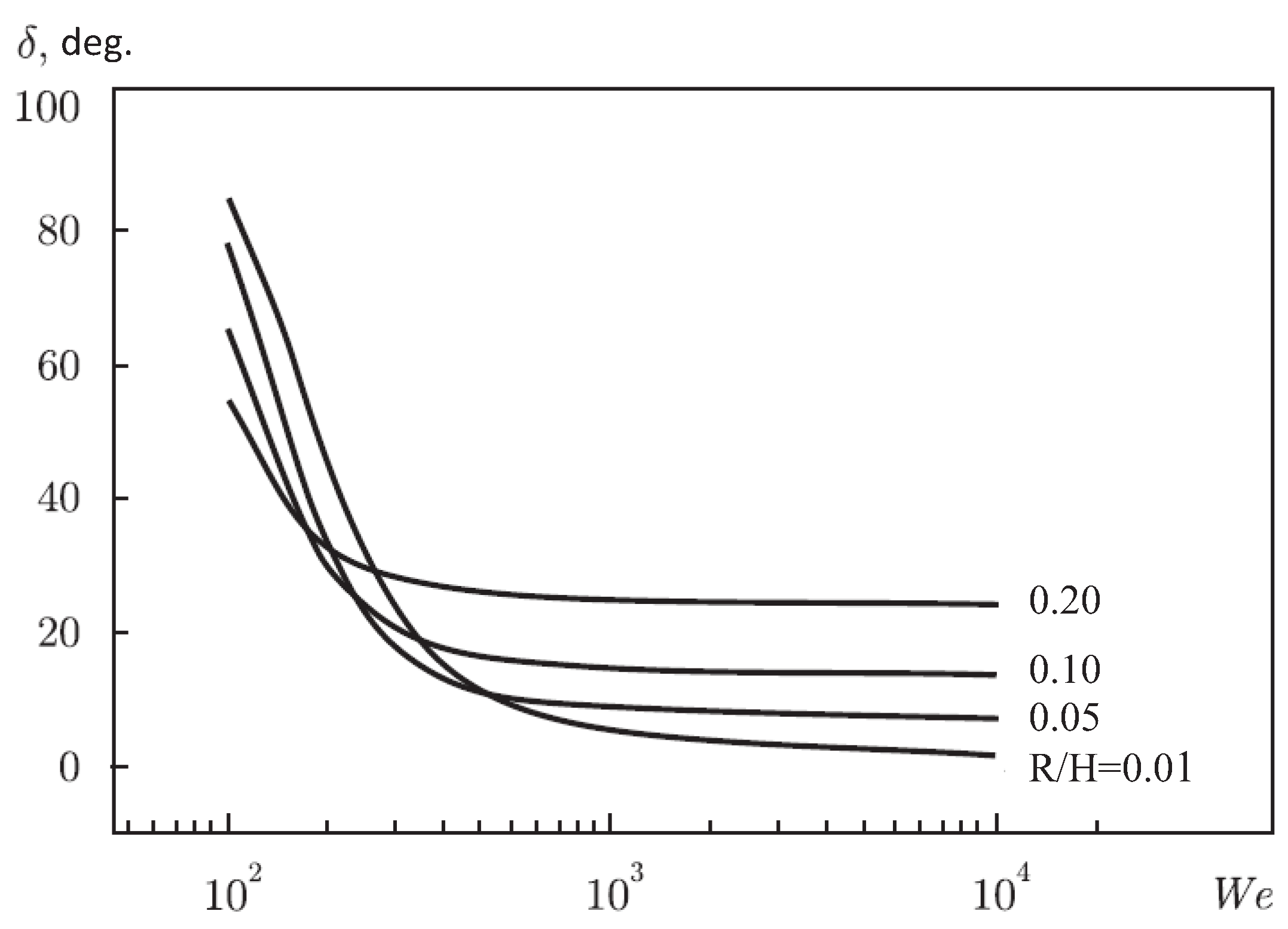
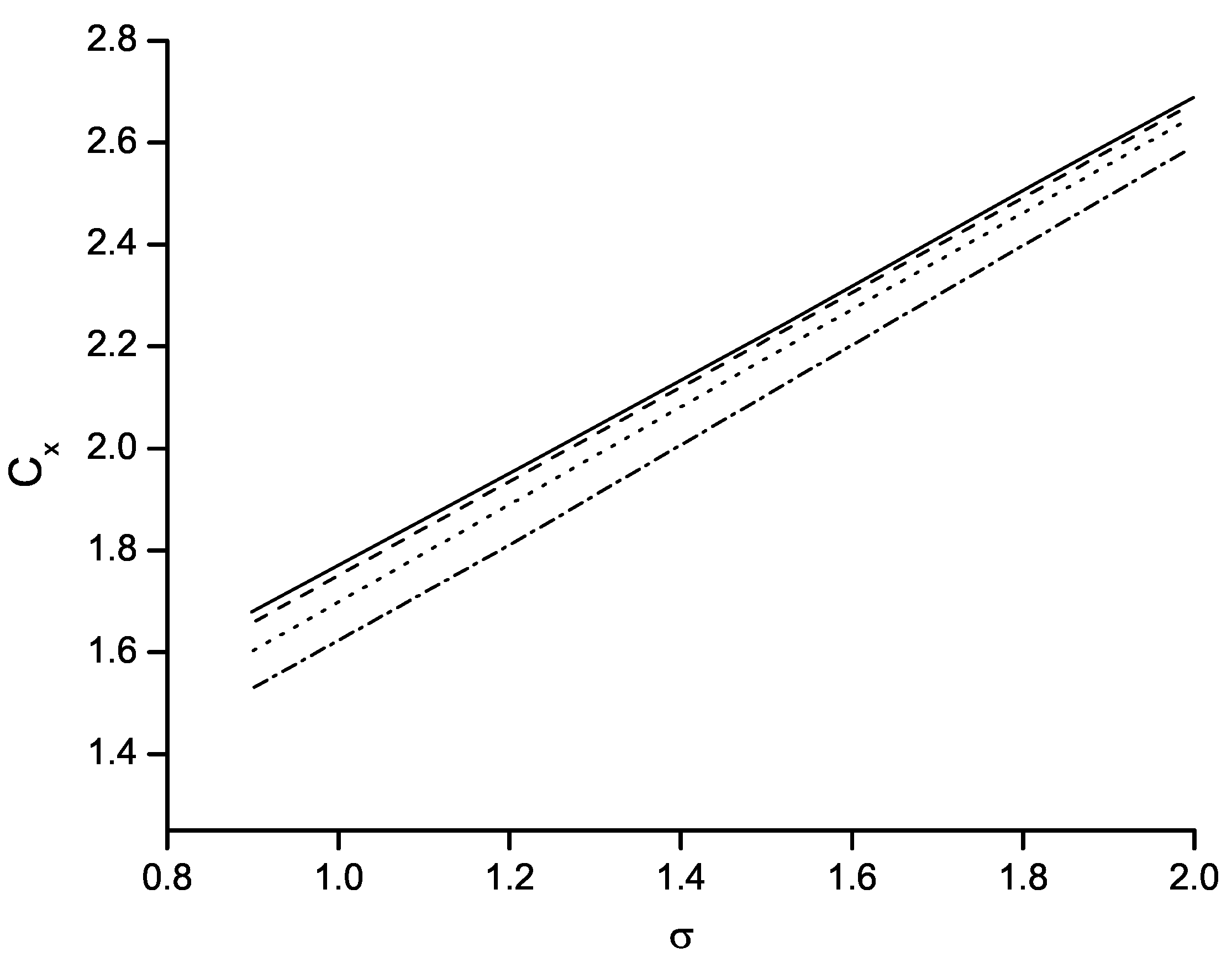
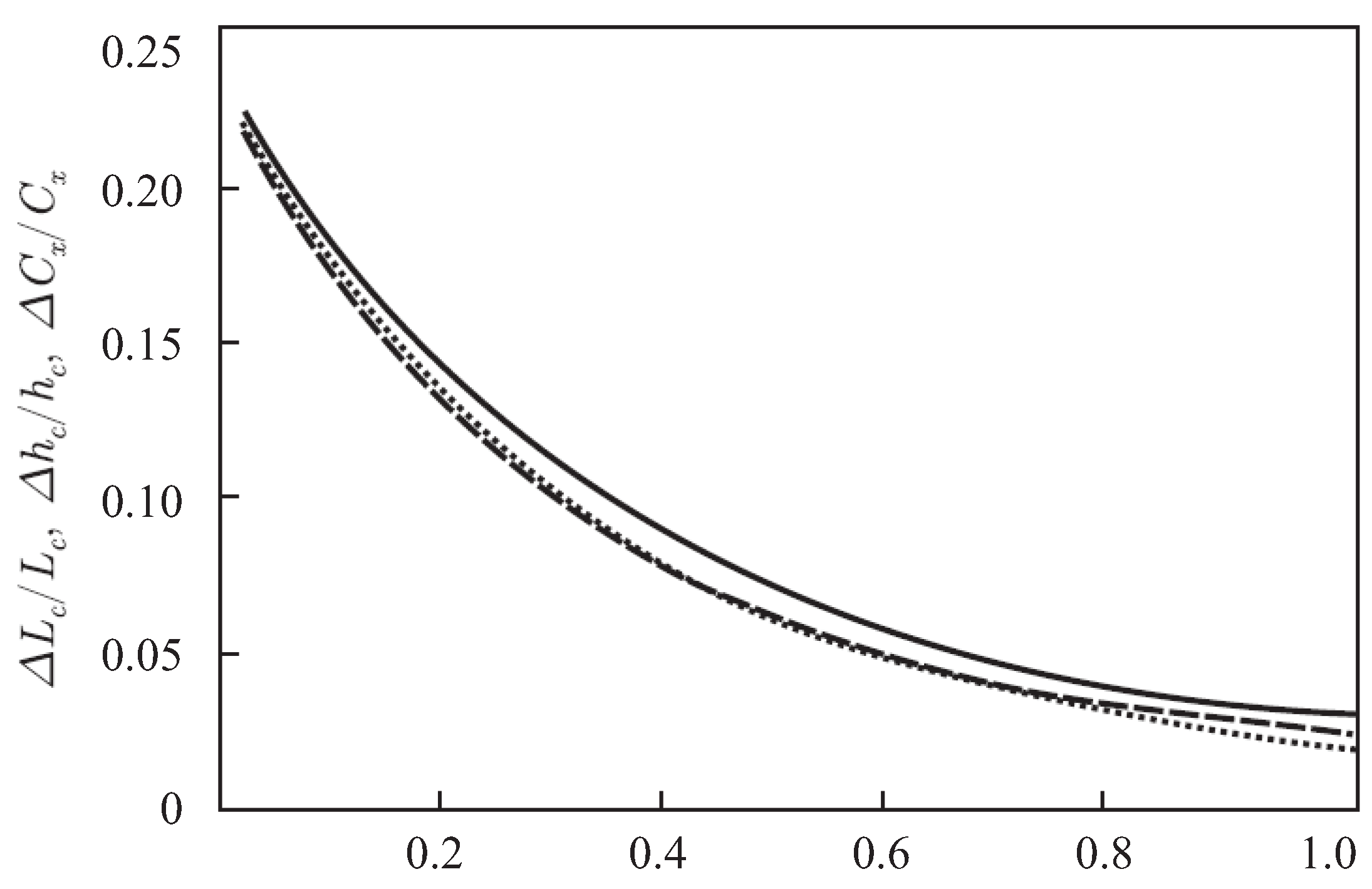
A case study is presented for a flat plate with rounded edges. The solution made it possible to determine the range of applicability of the model, which depends on the radius of the edges and the Weber number. For moderate Weber numbers, the surface tension slightly decreases the size of the cavity and the drag force. As the Weber number decreases further, the velocity at the point of cavity detachment increases, and the angle of flow detachment changes in such a manner that the wetting part of the edge becomes larger. The tendency seems to be towards to wetting the whole of the edge and making the flow attached to the wedge. However, this situation is not observed in the results due to the iteration process failing to converge for Weber numbers below some critical value. In these cases, a steady flow solution cannot be obtained. A similar situation occurs when the wedge radius tends to zero at some fixed value of the Weber number. The results obtained suggest that at Weber numbers below the critical value, the flow may become unsteady, and the point of cavity detachment may oscillate about some position on the edge. To verify this mechanism of cavity detachment, an advanced formulation of the problem, including flow unsteadiness and a more sophisticated flow model, are needed.

References

1. Brillouin, M. Les surfaces de glissement de Helmholtz et la resistance des fluids. Ann. Chim. Phys. 1911, 23, 145–230. [Google Scholar]
2. Villat, H. Sur la validite des solutions de certains problemes d’hydrodynamique. J. Math Pure Appl. 1914, 20, 231–290. [Google Scholar]
3. Yoon, B.S.; Semenov, Y.A. Capillary cavity flow past a circular cylinder. Eur. J. Mech. B/Fluids 2009, 28, 670–676. [Google Scholar] [CrossRef]
4. Birkhoff, G.; Zarantonello, E.H. Jets, Wakes and Cavities; Academic Press: New York, NY, USA, 1957. [Google Scholar]
5. Gurevich, M.I. Theory of Jets in Ideal Fluids; Academic Press: New York, NY, USA, 1965. [Google Scholar]
6. Vanden-Broeck, J.-M. The influence of surface tension on cavitating flow past a curved obstacle. J. Fluid Mech. 1983, 133, 255–264. [Google Scholar] [CrossRef]
7. Vanden-Broeck, J.-M. Nonlinear capillary free-surface flows. J. Eng. Math. 2004, 50, 415–426. [Google Scholar] [CrossRef]
8. Ackerberg, R.C. The effects of capillarity on free-stream line separation. IBID 1975, 70, 333–352. [Google Scholar]
9. Cumberbatch, E.; Norbury, J. Capillarity modification of the singularity at a free-streamline separation point. J. Mech. Appl. Maths. 1979, 32, 303–312. [Google Scholar] [CrossRef]
10. Yoon, B.S.; Semenov, Y.A. Cavity detachment on a hydrofoil with the inclusion of surface tension effects. Eur. J. Mech. -B/Fluids 2011, 30, 17–25. [Google Scholar] [CrossRef]
11. Bouwhuis, W.; Snoeijer, J.H. The effect of surface wettability on inertial pouring flows. arXiv 2015, arXiv:1507.05931. [Google Scholar]
12. Ni, B.Y.; Pan, Y.T.; Yuan, G.Y.; Xue, Y.Z. An experimental study on the interaction between a bubble and an ice floe with a hole. Cold Reg. Sci. Technol. 2021, 187, 103281. [Google Scholar] [CrossRef]
13. Yuan, G.Y.; Ni, B.Y.; Wu, Q.G.; Xue, Y.Z.; Zhang, A.M. An experimental study on the dynamics and damage capabilities of a bubble collapsing in the neighborhood of a floating ice cake. J. Fluids Struct. 2020, 92, 102833. [Google Scholar] [CrossRef]
14. Ho, C.-M.; Tai, Y.-C. Micro-electro-mechanical-systems (MEMS) and fluid flows. Annu. Rev. Fluid Mech. 1998, 30, 579. [Google Scholar] [CrossRef] [Green Version]
15. Gravesen, P.; Branegjerg, J.; Jensen, O.S. Microfluidics—A review. J. Micromech. Microeng. 1993, 3, 168. [Google Scholar] [CrossRef]
16. Mishra, C.; Pelesa, Y. Cavitation in flow through a micro-orifice inside a silicon microchannel. Phisics Fluids 2005, 17, 013601. [Google Scholar] [CrossRef]
17. Ghorbani, M.; Sadaghiani, A.K.; Villanueva, L.G.; Kosar, A. Hydrodynamic cavitation in microfluidic devices with roughened surfaces. J. Micromech. Microeng. 2018, 28, 075016. [Google Scholar] [CrossRef]
18. Semenov, Y.A.; Iafrati, A. On the nonlinear water entry problem of asymmetric wedges. J. Fluid Mech. 2006, 547, 231–256. [Google Scholar] [CrossRef]
19. Semenov, Y.A.; Yoon, B.S. Onset of flow separation at oblique water impact of a wedge. Phys. Fluids 2009, 21, 112103-1. [Google Scholar] [CrossRef]
20. Chaplygin, S.A. On the Pressure of a Plane Flow on Obstructing Bodies (To the Theory of an Airplane); Moscow University: Moscow, Russia, 1910; 49p. [Google Scholar]
21. Pilipenko, V.V.; Semenov, Y.A.; Pilipenko, O.V. Study of hydrodynamic cavitation in inducer centrifugal pumps. In Proceedings of the Third International Symposium on Cavitation, Grenoble, France, 7–10 April 1998; Volume 1, pp. 323–328. [Google Scholar]
22. Semenov, Y.A.; Tsujimoto, Y. A cavity wake model based on the viscous/inviscid interaction approach and its application to non-symmetric cavity flows in inducers. Trans. ASME J. Fluids Eng. 2003, 125, 758–766. [Google Scholar] [CrossRef]
23. Michell, J.H. On the theory of free stream lines. Phil. Trans. R. Soc. Lond. A 1890, 181, 389–431. [Google Scholar]
24. Joukovskii, N.E. Modification of Kirchhof’s method for determination of a fluid motion in two directions at a fixed velocity given on the unknown streamline. Math. Sbornik. 1890, 15, 121–278. [Google Scholar]
25. Anevlavi, D.; Belibassakis, K. An adjoint optimization prediction method for partially cavitating hydrofoils. J. Mar. Sci. Eng. 2021, 9, 976. [Google Scholar] [CrossRef]
26. Voskoboinick, V.A.; Grinchenko, V.T.; Makarenkov, A.P. Pseudo-Sound Behind an Obstacle on a Cylinder in Axial Flow. Int. J. Fluid Mech. Res. 2005, 32, 488–510. [Google Scholar] [CrossRef]
27. Andreev, M.V.; Drobakhin, O.O.; Saltykov, D.; Gorev, N.B.; Kodzhespirova, I.F. Simple technique for biconical cavity eigenfrequency determination. Radioelectron. Commun. Syst. 2017, 60, 555–561. [Google Scholar] [CrossRef]
28. Andreev, M.V.; Drobakhin, O.O.; Saltykov, D.; Gorev, N.B.; Kodzhespirova, I.F. Determination of biconical cavity eigenfrequencies using method of partial intersecting regions and approximation by rational fractions. Radioelectron. Commun. Syst. 2019, 62, 630–641. [Google Scholar] [CrossRef]
29. Semenov, Y.A. Nonlinear flexural-gravity waves due to a body submerged in the uniform stream. Phys. Fluids 2021, 33, 052115. [Google Scholar] [CrossRef]
Figure 1. Flow sketch: (a) physical plane (b) parameter, or ζ -plane.
Jmse 09 01253 g001
Figure 2. Cavity contours for various Weber numbers for edge radius r = 0.05 and cavitation number: (a) σ = 1.0 and (b) σ = 0.5 .
Jmse 09 01253 g002
Figure 3. Angle of the wetted part of the edge versus the Weber number for cavitation number σ = 1.0 and various edge radii.
Jmse 09 01253 g003
Figure 4. Drag force coefficient versus the cavitation number for radius r = 0.01 and Weber numbers: W e = 1000 (solid line); W e = 250 (dashed line); W e = 150 (dotted line); and W e = 100 (dot-dashed line).
Jmse 09 01253 g004
Figure 5. Relative difference of the cavity width (solid line), length (dashed line), and force coefficient (dotted line) for Weber numbers W e = 2000 and W e = 200 , versus the cavitation number. The edge radius is r = 0.02 .
Jmse 09 01253 g005
Publisher’s Note: MDPI stays neutral with regard to jurisdictional claims in published maps and institutional affiliations.