Article

An FTC Design via Multiple SOGIs with Suppression of Harmonic Disturbances for Five-Phase PMSG-Based Tidal Current Applications

1
Department of Electrical Automation, Shanghai Maritime University, Shanghai 201306, China
2
IREENA Laboratory, University of Nantes, 44602 Saint-Nazaire, France
*
Author to whom correspondence should be addressed.
J. Mar. Sci. Eng. 2021, 9(6), 574; https://doi.org/10.3390/jmse9060574
Submission received: 27 April 2021 / Revised: 23 May 2021 / Accepted: 24 May 2021 / Published: 26 May 2021

Abstract

:
This paper firstly adopts a fault accommodation structure, a five-phase permanent magnet synchronous generator (PMSG) with trapezoidal back-electromagnetic forces, in order to enhance the fault tolerance of tidal current energy conversion systems. Meanwhile, a fault-tolerant control (FTC) method is proposed using multiple second-order generalized integrators (multiple SOGIs) to further improve the systematic fault tolerance. Then, additional harmonic disturbances from phase current or back-electromagnetic forces in original and Park’s frames are characterized under a single-phase open condition. Relying on a classical field-oriented vector control scheme, fault-tolerant composite controllers are then reconfigured using multiple SOGIs by compensating q-axis control commands. Finally, a real power-scale simulation setup with a gearless back-to-back tidal current energy conversion chain and a small power-scale laboratory prototype in machine side are established to comprehensively validate feasibility and fault tolerance of the proposed method. Simulation results show that the proposed method is able to suppress the main harmonic disturbances and maintain a satisfactory fault tolerance when third harmonic flux varies. Experimental results reveal that the proposed model-free fault-tolerant design is simple to implement, which contributes to better fault-tolerant behaviors, higher power quality and lower copper losses. The main advantage of the multiple SOGIs lies in convenient online implementation and efficient multi-harmonic extractions, without considering system’s model parameters. The proposed FTC design provides a model-free fault-tolerant solution to the energy harvested process of actual tidal current energy conversion systems under different working conditions.

1. Introduction

Compared with classical three-phase rotating generators, multiphase generators [1] have irreplaceable merits, such as better fault tolerance, lower fluctuations and more degrees of control freedom. In recent years, the multiphase generators became a promising solution for tidal current applications, mainly due to the high fault tolerance as system operations in hash sea water environments require greater reliability and availability. For instance, by a five-phase permanent magnet synchronous generator (PMSG) studied in this paper, tidal current energy conversion systems (TCECS) with a most-used back-to-back conversion chain via a horizontal-axis turbine can be configured as the following three designs in Figure 1 according to the convenience of submarine maintenance. Figure 1a integrates the whole conversion chain under sea and transmit obtained powers to grid networks via submarine cables, which is the most general structure that can directly adapt to classical power generation systems. Figure 1b respectively separates five-phase machine side and three-phase grid side into offshore and onshore, linking by submarine cables. This architecture is a promising one that can be used for attractive direct current (DC) microgrid techniques and conveniently integrated with multi-source energies via DC grids, such as from photovoltaic, wind, waves, ocean thermal, etc., in offshore circumstances. Figure 1c only conserves the tidal current turbine and five-phase PMSG under sea and the other parts are installed onshore, which minimizes the maintained tasks in sea water. It can be seen that no matter what interrogation is adopted, the five-phase PMSG is always submarine placed, which increases the difficulties of maintenance and makes the generator more vulnerable to the harsh environment, even with fault occurrences. Thus, the reliability and availability of five-phase PMSG should be emphasized.
The placed five-phase PMSG is able to contribute more reliability and availability for the conversion chains since it has higher structural redundancies relative to classical three-phase generators. Its main advantage is that it can still operate with a degraded mode when one or two phases are absent [2,3]. In practice, the phase losses are mainly attributed to disconnected phase windings, fails of rectifier leg or isolating actions of the protectors. Nevertheless, once a phase-loss situation occurs, this leads to inter-phase imbalances in post-fault operations. For this reason, oversized torque ripples, high level vibrations and noise pollution become unfavorable factors in the whole power generation system [4,5]. Developing FTC algorithms aiming at the open circuit of the phase(s) are necessary for the five-phase PMSG-based TCECS.
According to operating mechanisms, the FTC algorithms can be categorized into active and passive types [6,7]. By means of information from the process fault diagnosis or fault estimation, the former type is mainly achieved via reorganization and reconfiguration of control laws or system model [8,9]. The active FTC algorithms are able to achieve complete fault restoration of a system and they have flexible design procedures, while the accuracy of fault information is a prerequisite [10]. The fault diagnosis/estimation stage also causes computational burden. From [2,10,11], rules of coordinate transformations are actively reconfigured to conserve the orthogonality only in the principal sub-space, eliminating the rest of components in stationary frames. The generalization of these algorithms is constrained as they are effective only for the preset fault types [9,12]. The last drawback of active FTC algorithms lies in the effects of interaction between fault diagnosis/estimation and the FTC, which is illustrated in [12]. Therefore, the passive FTC algorithms are still worth being studied as they are inspired by classical robust control methods that concern only the sensitivity level of a fault instead of a fault’s size and location. Conventionally, this kind of passive FTC algorithm treats the fault or the failure as a kind of disturbance or a unmodeled uncertainty (see [13,14]), of which there is an abundant amount of theory on in the past five decades. Even so, the classical passive FTC algorithms are vulnerable to modelling complexities, parameters setting and a lack of explanatory mechanisms. The passive FTC has an obvious limitation to obtain satisfactory fault tolerance compared with the active one. Regarding the popular hybrid solutions around the studied issue in this paper, there emerged several representative research works. Liu et al. [15] designed an active FTC strategy combining fault status and fault compensation based on a disturbance observer-based method. The fault compensation can handle all the situations theoretically that characterize the features of passive FTC. Kiselev et al. [16] proposed a robust fault tolerant method by model predictive control based on a finite control set. This is similar to the passive FTC, as the fault detection is also provided by the predicted variables. Azizi et al. [17] designed an active FTC method based on the robust sliding mode observers, which involves intuitive fault estimation and compensation. From the mentioned works, the modelling complexities, assistance of fault information as well as facilitation of implementation of the FTC algorithm should be synthetically considered with a view of tradeoff.
By the aforementioned discussions, a multiple second-order generalized integrators (multiple SOGIs) [18] based FTC strategy is proposed in this paper and applied into the five-phase PMSG-based TCECS. The PMSG contains trapezoidal back-electromagnetic forces (back-EMFs), and the single-phase open condition is investigated carefully. Different from the usage into grid synchronizations as [18], multiple SOGIs innovatively characterize the model-free fault estimator by extracting the main harmonic disturbances, relative to the similar model-based fault estimators [15,19,20,21,22,23].
It is worth pointing out that this work provides a more flexible design and it is independent to system modelling, via a compensation mechanism of selective harmonic, compared with our recently published model-based FTC strategy [15]. Compared with notch-filters-based [24] and proportional-resonant-based methods [25], this multiple SOGIs based strategy is convenient for designing multi-resonant compensators for online implementations with less parameter setting. This proposal integrates the thoughts of fault estimation from the active FTC methods and the independence of fault’s prior knowledge from the passive FTC ones. The modelling of additional harmonics is also carefully investigated under the condition of single-phase open. Finally, the feasibility and performance of the proposed method are verified by a real power-scale simulation setup with a direct-driven five-phase PMSG and a small power-scale laboratory prototype emulating TCECS in machine side. The main objective of this research is to develop a feasibly convenient technique to improve the capability of anti-interferences and fault tolerance for the TCECS, making it adapt to both healthy modes and the malfunctioned conditions.
The remainder of this paper is summarized as follows. Section 2 details system modelling and problem formulation. The proposed multiple SOGIs based model-free FTC strategy is illustrated in Section 3. Based on a real power scale simulation setup, Section 4 demonstrates the advantages of five-phase PMSG over the three-phase one and tests the effectiveness of the proposed FTC method for five-phase PMSGs with different trapezoidal degrees. Section 5 analyzes the mechanism with a deeper study via harmonic spectrum analysis based on experimental tests. Finally, Section 6 concludes this work.

2. System Modeling and Problem Formulation

According to the back-to-back structure illustrated as Figure 1, the following aspects are indicated and assumed in the modelling and the problem formulation:
  • Swell effects and turbulences are not considered for the tidal current speed;
  • Only the 1st and 3rd harmonic components in back-EMFs are considered;
  • Harmonic disturbances are discussed under a single-phase open case;
  • The permanent magnets are surface mounted on the rotor of the five-phase PMSG used in the simulation setup and the laboratory prototype;
  • Magnetic curve is linear;
  • Eddy currents, iron losses are negligible;
  • Stator phase windings are star-connected and neutral wire is absent.

2.1. Model of Tidal Current Turbine

A horizontal-axis tidal current turbine integrated with a five-phase PMSG is adopted to harness the electrical power from tidal current energies. The acquired hydrodynamic energy [26] of the tidal current turbine can be calculated by:
P t u r = 0.5 ρ π r 2 ν t i d e s 3 C p
where ρ represents the weight density of sea water, νtides means tidal current speed of, and r indicates the radius of turbine blade. Cp, the power coefficient of the turbine, depends on the tip speed ratio (TSR, λ=ωturr/νtides) and pitch angle β, where ωtur represents the angular velocity of tidal current turbine. Here, the Cp also suffers from an upper bound (around 59.3%) through such a horizontal-axis tidal current turbine by Betz’s law [27]. A three-dimensional Cp graphics is thus depicted as shown in Figure 2, which can be calculated as Equation (2).
Figure 2. The graphics of Cp (λ, β).
Jmse 09 00574 g002
C p ( λ , β ) = C 1 C 2 λ i C 3 β C 4 e C 5 λ i i + C 6 λ i i λ i i = 1 / 1 λ + 0.008 β 0.003 β 3 + 1
where C1~C6 are coefficients of Cp (λ, β) function, which are given in Table 1. λii represents the intermediate variable of the TSR.
According to the above Cp curve, the maximum powers and optimal torques excited by tidal current through the turbine can be thus given by:
P t u r _ max = ρ π r 5 C p max 2 λ opt 3 ω t u r 3 T t u r _ opt = P m _ max ω t u r
where the optimal TSR and maximum power coefficient are, respectively, denoted as λopt (6.545) and Cpmax (0.44335).
From Equation (3), it can be seen that the maximum powers and optimal torque are respectively proportional to cubic and square of the velocity ωtur, whose operational characteristics can be shown in Figure 3 (Ttur-ωtur). It can be obvious to see that the optimal torque curve doesn’t pass through the points of maximum torque. The reason is that the maximum torque points correspond to the maximum powers, while the optimal torque is equal to that the maximum power divided by the mechanical speed as described in Equation (3).
In this paper, only the maximum power point tracking (MPPT) process is discussed below the rated power, where the pitch angle β is 0°. The optimal torque points in Figure 3 are thus only presented in the part between the cut-in speed (1 m/s) and the rated speed (3.2 m/s). On the purpose of optimal control of the MPPT process, the reference of optimal ωtur can be given by:
ω t u r * = ν t i d e s λ opt / r
Figure 3. Ttur-ωtur curves under various velocities.
Jmse 09 00574 g003

2.2. Mechanical Model of Drive Train

The gear ratio between the tidal current turbine and five-phase PMSG is defined as Ngear (Ngear = ωtur/ωm), where ωm represents the mechanical angular velocity of the generator. It is worth knowing that the equivalent gear ratio in the small power-scale laboratory prototype is greater than 1 with the tidal current turbine. The real power-scale simulation setup makes use of a gearless type (Ngear = 1). The mechanical coupling structures of the drive train are shown in Figure 4a,b. Particularly, the torsional damper is used to reduce variations of rotated shafts. The rigid coupling shafts and gears maintain the consistent angular velocities and angles of the inputs and outputs while there is a non-negligible angle shift (defined as θΔtd) of the torsional dampers with flexible coupling structures.
In Figure 4a, the dynamics of turbine shaft, torsional damper and generator shaft can thus be modeled as:
J t u r ω ˙ m = T t u r T t u r 1 B t u r ω m T m = T t u r 2 N g e a r = T t u r 1 N g e a r = K t d θ Δ + B t d θ ˙ Δ , θ Δ t d = θ t u r J g e n ω ˙ m = T m T e B g e n ω m θ m N g e a r
where Jtur and Jgen represent the inertia of the turbine and the generator, respectively. Btur, Btd and Bgen represent friction coefficients in the turbine’s shaft, torsion damping coefficient and the generator’s shaft, respectively. Mechanical and electromagnetic torques of the generator are denoted as Tm and Tem. The torque term Ttur1 is a discounted one relative to Ttur, passing the turbine shaft, where Ttur1 = Ttur2 = NgearTm. In the second sub-equation, Ktd is the strength of anti-torsion for the torsional damper. It should be pointed out that the Btur, Btd and Bgen represent the lumped frictions by using slide bearings or roller bearings. For the gearless or so-called direct driven type in Figure 4b, the only difference is to remove the gearbox, whose model can be obtained as a special case in Equation (5), substituting Ngear by 1. In this paper, the effects of torsional dampening are neglected, assuming the shafts are well coupled to each other.

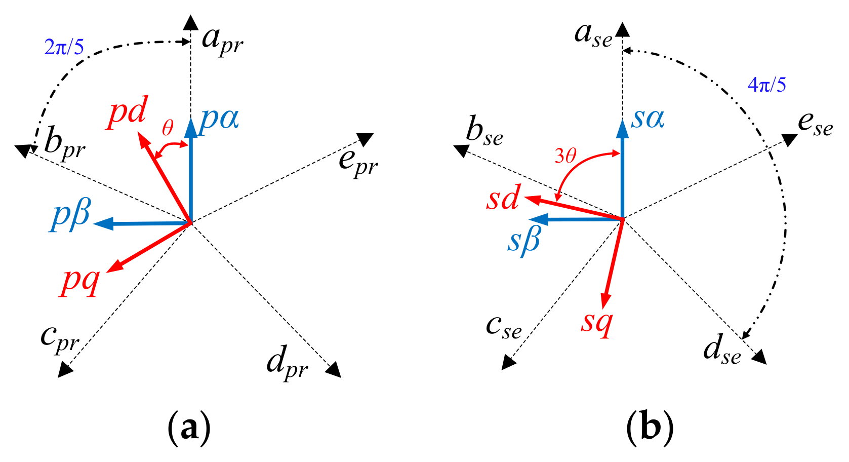
2.3. Modeling of Five-Phase PMSG in Healthy Conditions

Electrical voltage equations [28] of the stator windings in the original frame are thus given by:
v a v b v c v d v e = e a e b e c e d e e R s i a i b i c i d i e L s M 1 M 2 M 2 M 1 M 1 L s M 1 M 2 M 2 M 2 M 1 L s M 1 M 2 M 2 M 1 M 2 M 2 M 1 M 2 L s M 1 M 1 L s d d t i a i b i c i d i e
where vx, ex and ix (x = a, b, c, d, e) are, respectively, the phase voltages, back-EMFs and phase current. Ls is the self-inductance of the stator windings. M1 and M2 are mutual inductances of the adjacent and non-adjacent phases, respectively. In this paper, the resistances of five phase stator windings are assumed the same for each the winding as Rs. The back-EMFs of the generator contains 1st and 3rd harmonic components, which can be expressed as:
e a e b e c e d e e = p ω m Φ 1 sin p ω m t + φ 1 sin p ω m t 2 π / 5 + φ 1 sin p ω m t 4 π / 5 + φ 1 sin p ω m t 6 π / 5 + φ 1 sin p ω m t 8 π / 5 + φ 1 + 3 p ω m Φ 3 sin 3 p ω m t + φ 3 sin 3 p ω m t 2 π / 5 + φ 3 sin 3 p ω m t 4 π / 5 + φ 3 sin 3 p ω m t 6 π / 5 + φ 3 sin 3 p ω m t 8 π / 5 + φ 3
where p is the number of pole pairs and ωm is mechanical angular velocity of five-phase PMSG. Φ1 and Φ3 represents the magnet fluxes yielded by the stator windings corresponding to the fundamental and 3rd harmonic components of the back-EMFs, respectively. φ1 and φ3 are defined as the corresponding initial phase angles. By a generalized Concordia transformation depicted in Figure 5, the five phase PMSG can be decomposed into three sub-generators, the principal, the secondary and the homopolar ones corresponding to three sub-spaces. Since the neutral wire is not connected and the stator windings are star-connected, the last sub-generator will be not available in healthy mode. In the principal sub-space, the original, Concordia’s and Park’s frames can be indicated by different axes with (apr, bpr, cpr, dpr, epr), (, ) and (pd, pq). Similarly, the three frames in the secondary sub-space are expressed by the axes (ase, bse, cse, dse, ese), (, ) and (sd, sq), respectively.
Relying on the above orthogonal transformations, vectors in Equation (6) can be projected into stationary frames by a generalized Park transformation shown in Figure 5.
Using a Park’s transformation matrix for trapezoidal back-EMFs Equation (A1) in Appendix A, the stator voltage equation is thus written as:
v p d = e p d R s i p d L p r d i p d d t + p ω m L p r i p q v p q = e p q R s i p q L p r d i p q d t p ω m L p r i p d ( Primary   sub space ) v s d = e s d R s i s d L s e d i s d d t + 3 p ω m L s e i s q v s q = e s q R s i s q L s e d i s q d t 3 p ω m L s e i s d ( Sec ondary   sub space )
where Lpr and Lse represent equivalent inductances for principal and secondary sub-generators, respectively. vz, ez and iz (z = pd, pq, sd, sq) are respectively phase voltages, back-EMFs and phase current under Park’s frames.
Besides, electromagnetic torque is then deduced by:
T e m = i p d e p d + i p q e p q + i s d e s d + i s q e s q ω m

2.4. Modelling of Five-Phase PMSG with Single-Phase Open

With the symmetrical winding structure, the five-phase voltages and currents in healthy condition can be expressed as:
x = a , b , c , d , e v x = 0 , x = a , b , c , d , e i x = 0
On the basis of the above model under healthy conditions, we can assume that phase “a” is open here. The above Equation (10) is then modified as:
x = a , b , c , d , e v x = 0 ,   i b + i c + i d + i e = 0
In this condition, the voltages in healthy phases can be found by using the voltage potential of the neutral point in the associated converter legs, that is:
v b = u b u N o v c = u c u N o v d = u d u N o v e = u e u N o
By Equations (11) and (12), the voltage at neutral point of the DC link is deduced into
u N O = u b + u c + u d + u e + v a 4
where subscript “N” and “O” represent the neutral node of the star-connected stator winding and neutral point in the DC link with the MSC. The output voltage va in the opened phase is expressed as:
v a = e a M 1 d i b d t + d i e d t M 2 d i c d t + d i d d t
Substituting Equations (10)–(13), the overall voltage equation can be deduced as:
V = E R s I L d d t I
where the new matrices are expressed as:
V = 1 4 3 1 1 1 1 3 1 1 1 1 3 1 1 0 1 1 u b u c u d u e , I = i b i c i d i e T , E = e b + 1 4 e a e c + 1 4 e a e d + 1 4 e a e e + 1 4 e a T L = L s + 1 4 M 1 M 1 + 1 4 M 2 M 2 + 1 4 M 2 M 2 + 1 4 M 1 M 1 + 1 4 M 1 L s + 1 4 M 2 M 1 + 1 4 M 2 M 2 + 1 4 M 1 M 2 + 1 4 M 1 M 1 + 1 4 M 2 L s + 1 4 M 2 M 1 + 1 4 M 1 M 2 + 1 4 M 1 M 2 + 1 4 M 2 M 1 + 1 4 M 2 L s + 1 4 M 1
When open circuit occurs at single phase of the five-phase PMSG, its symmetrical structure is broken, which then causes significant unbalance among phases. For instance, it can be observed from above expression that the inductance matrix has been changed after fault occurrences. The back-EMFs in the remaining healthy phases will be added with 1/4 times of ea. Then, the back-EMFs under the single-phase open condition can be expressed as:
E = p ω m Φ 1 sin p ω m t 2 π / 5 + sin p ω m t 4 sin p ω m t 4 π / 5 + sin p ω m t 4 sin p ω m t 6 π / 5 + sin p ω m t 4 sin p ω m t 8 π / 5 + sin p ω m t 4 + 3 p ω m Φ 3 sin 3 p ω m t 2 π / 5 + sin 3 p ω m t 4 sin 3 p ω m t 4 π / 5 + sin 3 p ω m t 4 sin 3 p ω m t 6 π / 5 + sin 3 p ω m t 4 sin 3 p ω m t 8 π / 5 + sin 3 p ω m t 4

2.5. Additional Harmonic Disturbances Subject to Single-Phase Open

In general, copper losses for a certain torque are indicated by:
P c o p p e r = R s ( i p q 2 + i p d 2 + i s q 2 + i s d 2 )
The above current norm is minimum only if the current vectors and back-EMF vectors satisfy Fleming’s right-hand rule [29]. In other words, their relationships can be collinear to achieve the minimize copper losses, which is expressed as below without considering higher order back-EMF harmonic components.
i s q i p q = e s q e p q = 3 Φ 3 Φ 1 = X r
Substituting Equations (8) and (17), the desired current references are given by:
i p d * = 0 ,   i p q * = e p q e p d 2 + e p q 2 T e m * ω m = T e m * / K t = T e m * / 5 2 p Φ 1 1 + X r 2 i s d * = 0 ,   i s q * = X r i p q *
where Kt represents the conversion gain from torque to current references. The references in Equation (18) are convenient for controlling principal and secondary sub-generators.
By inverse Park transformation, the healthy phase current under control in abcde frames will be yielded as:
i x c t r ( t ) = 2 T e m * 5 p 1 + X r 2 Φ 1 X r sin 3 p ω m t 2 π 5 k 1 + sin p ω m t 2 π 5 k 1
where k = 1, 2, 3, 4, 5 represents the kth phase among phase ‘a’ to phase ‘e’.
Under faulty conditions, the symmetrical structure of five-phase PMSG will be broken and torque ripples will occur. The additional odd harmonic orders only need to be considered since the stator winding is star-connected [30]. For simplifications, we can assume that the single-phase open occurs at phase ‘a’ and the distorted phase current in original abcde frames contained 1st, 3rd, 5th and 7th harmonic disturbances. Similar to Equation (19), their expressions of phase current under the single-phase open condition can be organized as:
i a ( t ) i b ( t ) i c ( t ) i d ( t ) i e ( t ) = 2 T e m * 5 p 1 + X r 2 Φ 1 0 h = 1 , 3 , 5 , 7 η b h sin h p ω m t 2 π 5 + θ b h h = 1 , 3 , 5 , 7 η c h sin h p ω m t 4 π 5 + θ c h h = 1 , 3 , 5 , 7 η d h sin h p ω m t 6 π 5 + θ d h h = 1 , 3 , 5 , 7 η e h sin h p ω m t 8 π 5 + θ e h
where h represents the number of harmonic orders in phase current. ηbh means the amplitude ratio of hth harmonic order in the current of phase “b”. θbh is the phase shift of it relative to the phase angle in healthy conditions. The definition rules are the same in other phases. It should be noted that the phase shifts are constant and small in steady states, which are ignored here.
With the coordinate transformation as Equation (A1) in Appendix A, the phase current in Park’s frames is then projected as below.
i p d ( t ) i p q ( t ) i s d ( t ) i s q ( t ) i 0 _ d q ( t ) = 2 T e m * 5 p 1 + X r 2 Φ 1 T Park 13 0 h = 1 , 3 , 5 , 7 η b h sin h p ω m t 2 π 5 + θ b h h = 1 , 3 , 5 , 7 η c h sin h p ω m t 4 π 5 + θ c h h = 1 , 3 , 5 , 7 η d h sin h p ω m t 6 π 5 + θ d h h = 1 , 3 , 5 , 7 η e h sin h p ω m t 8 π 5 + θ e h
Relying on the above illustrations and deductions as Equations (A3) and (A4) in Appendix B, Table 2 present general descriptions of harmonic distributions for phase current or back-EMFs vectors. It can be seen that the additional harmonics mainly consist of even order additional harmonics in Park’s frames, especially the 2nd, 4th, 6th, 8th and 10th ones as shown in the equations in Appendix B through superposition theorem. Specifically, it can be observed that the principal sub-generator is affected by 2nd, 4th, 6th, 8th harmonic disturbances in the single-phase open condition. For the secondary sub-generator, 2nd, 4th, 6th, 8th and 10th harmonic components constitute the main harmonic disturbances. Similar to the harmonic analysis of the phase current, vectors of back-EMFs in Park’s frames also mainly consist of the corresponding even order fluctuations. Either for phase current or back-EMFs, these unexpected interferences should be suppressed comparing with their quantities in healthy operation modes.
Although the zeros sequence or the homopolar sub-generator is neglected, as mentioned earlier, it is worth knowing that this only holds true in a healthy condition. In faulty conditions, the harmonic content in zeros sequence or the homopolar sub-generator will no longer be equal to zeros, due to the unbalanced structure in the five-phase PMSG (here, the single-phase open fault will be discussed). For instance, the harmonic components in homopolar sub-generator are discussed in Table 2 and the equations in Appendix B.

3. Multiple SOGIs-Based Model-Free FTC Strategy

In order to precisely explore the process of harmonic compensation, a fault-tolerant control method is designed via a multiple SOGIs-based structure.

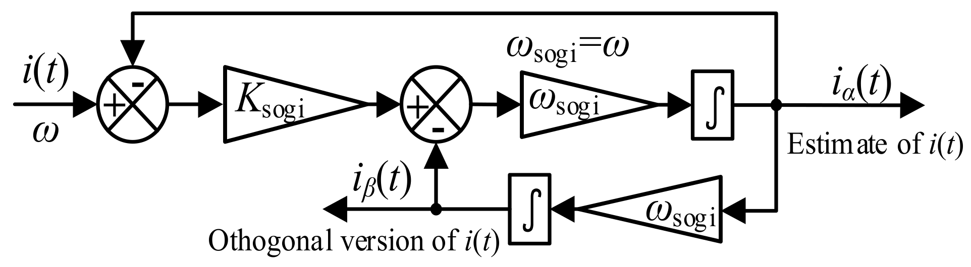
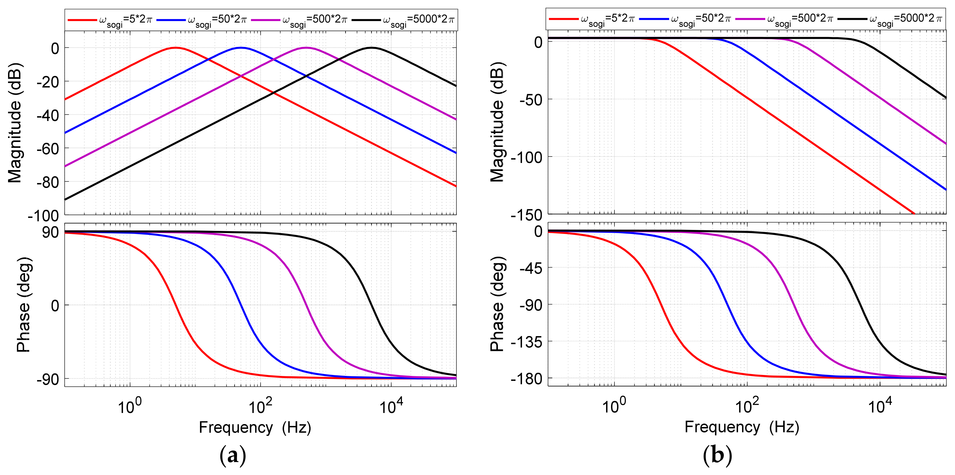
3.1. Single SOGI and Multiple SOGIs

Figure 6 is a classical structure of a single SOGI. Ksogi and ωsogi represent the filter gain and its resonant frequency, respectively. iα(t) and iβ(t) are output signals of the single SOGI.
Their transfer functions are deduced as:
F α ( s ) = I α ( s ) I ( s ) = K sogi ω sogi s s 2 + K sogi ω sogi s + ω sogi 2 , F β ( s ) = I β ( s ) I ( s ) = K sogi ω sogi 2 s 2 + K sogi ω sogi s + ω sogi 2
Figure 7 shows bode plots of the above equations, which are plotted under various filter gains Ksogi and resonant frequencies ωsogi. It can be observed from Figure 7a,b that the bandwidths of both Fα(s) and Fβ(s) are sensitive to the parameter Ksogi. A greater value of Ksogi brings a broader bandwidth around the resonant frequency but reduces the robustness of the SOGI [31]. On the contrary, a small Ksogi will narrow the bandwidth and slow down its dynamic responses. In this paper, Ksogi is fixed as 2 concerning the dynamic transient behaviors of the single SOGI. As the angular velocity of the input signal (ω) is equal to the resonant one of the single SOGI (ωsogi), iα(t) and iβ(t) can be regarded as an estimated term and an orthogonal version of the input signal, respectively. According to Figure 7a,b, the single SOGI is able to estimate a certain frequency as ωsogi varies.
For a compensation point of view, iα(t) is selected since it can estimate the input signal at a specific harmonic without phase shifts. However, for the concern of extension towards multiple harmonic orders, the above single frequency resonant based filter is clearly inadequate. As mentioned, a SOGI presents a stable characteristic for the selection of any frequency order from the input signal as shown in Figure 7a,b. A straight way for designing a multiple harmonic resonant structure is to establish a series of SOGI filters with different resonant frequencies in parallel. Similar to a single SOGI, the expression of multiple SOGIs [18] concerning on the lth order frequency can be organized as below using the transfer function Fα(s).
F multiple _ SOGIs _ l ( s ) = F α , l ( s ) j = 1 j l n 1 F α , l ( s ) 1 F α , l ( s ) F α , j ( s )
where Fα,j(s) represents the transfer function of a single SOGI with the estimation of the jth harmonic resonance. n means the number of harmonic orders, which is a positive integral term.
Consequently, a general topology of multiple SOGIs is illustrated as Figure 8a. When one frequency is captured from a signal superimposed with many harmonic orders, this kind of structure can effectively extract any specific harmonic orders by eliminating the mutual influences from other harmonics. The SOGI blocks with various resonant frequencies from ω to are able to, respectively, extract from 1st to nth harmonic components of the input signal i(t). For simplifications, the DC component of the input signal i(t) can be also obtained from the result after excluding the estimated harmonic orders (≥1) of i(t). Hence, the characteristic of frequency response of the single SOGI, multiple SOGIs and direct sum of SOGIs are indicated by the bode plot shown in Figure 8b. The diagram gives an example of the cancellation of frequencies from 2nd to 7th, conserving the fundamental frequency (here 50 Hz). Particularly the direct sum of SOGI blocks is not able to effectively avoid the mutual interferences from other harmonics. It is obvious that multiple SOGIs are able to extract this specific harmonic component with good accuracy and dynamic behaviors by decaying other harmonic orders, which facilitates the situations due to the interferences by multiple harmonic disturbances.

3.2. Multiple SOGIs-Based Model-Free FTC Design for Five-Phase PMSG-Based TCECS

According to the system structure described in Figure 1, the generator side converter can be modeled by a first-order delay Kpwm/(1+1.5Tpwms). The time constant of switching frequency and the equivalent gain of pulse width modulation (PWM) are defined as Tpwm and Kpwm, respectively. Vcarrier, the amplitude of carrier signals, is set as 1. The controller parameters [15] in inner current loops can be given by:
K p p d = K p p q = L p r 3 K p w m T p w m , K p p d = K p p q = L s e 3 K p w m T p w m K i p d = K i p q = K i s d = K i s q = R s 3 K p w m T p w m
The speed loop PI parameters are denoted as Kp and Ki.The classical control law of the dual-loop system can be expressed as:
i p q * = K p Ω + K i Ω s Ω * Ω
u p q * = K p p q + K i p q s i p q * i p q , u s q * = K p s q + K i s q s i s q * i s q
According to the optimal references in Equation (18), the electromagnetic torque described in Equation (8) can be rewritten as below with the two power-generation sub-systems.
T e m = T e m 1 + T e m 3 T e m 1 = i p q 5 2 p Φ 1 , T e m 3 = i s q 3 5 2 p Φ 3
where Tem1 and Tem3 represent the torque components with respect to the two power-generation sub-systems, which are respectively affected by the 1st and 3rd harmonics of the back-EMFs.
On the basis of above analysis, the control diagram related to q-axes in healthy conditions is designed as shown in Figure 9. The torque reference directly links to ipq and isq in inner control loops by the description from Equation (27). Thus, the harmonic compensation by multiple SOGIs is then integrated only in the two q-axis control loops. In order to keep the level of Tem, the estimate term of the DC component through the multiple SOGIs will not be injected to the isq and ipq control loops. In detail, the extracted harmonics from output control commands vpq* and vsq* are injected with self-feedback loops. It should be noted that the parameter variations are neglected here, such as the inductances illustrated in Equation (14). d-axis current control loops are expected to be controlled within zeros, where the disturbances are not currently considered as the q-axis current control loops determine the main amplitude of torque under the vector control framework. The epq and esq contain even order harmonics, as per the analysis in Section 2.2, which are considered as external disturbances that need to be compensated together with the fault harmonic disturbances as the single-phase open fault occurs.
Consequently, the fault-tolerant composite controllers in the q-axis current control loops can be expressed as:
v p q _ c o m p * = K p p q + K i p q s i p q * i p q + v h _ p q v s q _ c o m p * = K p s q + K i s q s i s q * i s q + v h _ s q
where vh_pq and vh_sq represent the injected harmonic disturbances to the control commands vpq* and vsq* in feedforward paths, respectively. The corresponding compensation gains are denoted as Kh_pq and Kh_sq.
Figure 9. Control diagram in q-axis current control loops with the multiple SOGIs-based compensations.
Jmse 09 00574 g009

4. Simulation Test by Real Power Scale Tidal Current Turbine Systems

According to the turbine and generator model described in Section 2, a 1.5 MW five-phase PMSG-based tidal current energy simulation setup is established under a MATLAB/SIMULINK (Release 2018a 64-bit for windows—MathWorks, Natick, MA, USA) environment. Figure 10 shows a landscape of a real-scale power simulation setup. Here, the five-phase PMSG is built by a Simscape framework and the other parts are organized through elements in Simpowersystem libraries. Composite controllers are reconfigured by multiple SOGIs-based compensators in q-axis current loops, presented as the marked shadow in red. The main parameters of the setup refer to [32], listed in Table A1 in Appendix A. This five-phase PMSG with trapezoidal back-EMFs contains a 1st harmonic and an additional third harmonic component. As mentioned in Section 2, this paper focuses on the MPPT process. Thus, working performance under variable tidal current speed profiles are investigated. Otherwise, multiple SOGIs-based compensation is the main metric to be studied in this paper. Its validation either in healthy and faulty conditions is carried out under a constant speed profile (νtides = 2.055 m/s). The other practical concern is that actual maintenance requests the implementation within the shortest possible duration.

4.1. Comparison of Performance Using Five-Phase and Three-Phase PMSG

Based on the 1.5 MW tidal current turbine model described in Section 2.1, the five-phase PMSG-based simulation setup can be compared with an equivalent three-phase PMSG-based one. According to the common theory of mathematical modelling, the only difference is the number of phases; other parameters remain the same. Since the machines’ phases are different, the MPPT characteristics described in Figure 2 and Figure 3 are not accessible anymore. Hence, the comparative studies were carried out under a condition of constant mechanical angular velocity (1.6812 rad/s) and constant input mechanical torque (0.2337 MN·m), which ensures the same power offered by the tidal current turbine, as the article [33] implemented. Including the DC bus, grid-side configurations and the control theory, these other parts are the same as the simulation schematic in Figure 10. To facilitate the comparisons, the tests were implemented under the most classical condition that only exists for sinusoidal back-EMFs for three- and five-phase PMSGs. The model for the five-phase PMSG in this condition was built in Park’s frames with the transformation matrix as Equation (A2), rather than the Equation (A1) in Appendix A. The three-phase PMSG uses the classical three-phase coordinate transformations.
The six sub-figures in Figure 11a show the mechanical angular velocities, torques, phase current of the three-phase PMSG-based system, phase current of the five-phase PMSG-based system, powers of the three-phase PMSG-based system and powers of the five-phase PMSG-based system. In detail, Figure 11a,b indicate that the five-phase PMSG has smaller speed fluctuations and torque ripples than the three-phase one. By decreasing the number of phases, the amplitudes of phase current in the three-phase PMSG are higher relative to an exploit of the five-phase PMSG, which are presented in in Figure 11c,d. The phase current signals in the five-phase PMSG are smoother than the three-phase one. In addition, the five-phase PMSG has superior performance in terms of powers’ perturbations in the machine side, DC bus and grid side, comparing the last two sub-figures.
The structure of more phases (the five-phase PMSG) brings smoother rotating operations, which ensure the whole power conversion chain is stable and without major fluctuations. In practice, this kind of operational characteristic also contributes to less pressure on the semiconductor switches in converters. This test verifies the merit of a five-phase PMSG compared with the classical three-phase PMSG. Since the third harmonic component in the trapezoidal back-EMFs is small, with respect to the fundamental one in this simulation setup, this comparative test in healthy conditions can also be used to make up the motivation for using five-phase PMSG rather than the three-phase one.

4.2. Test of Fault-Tolerant Performance
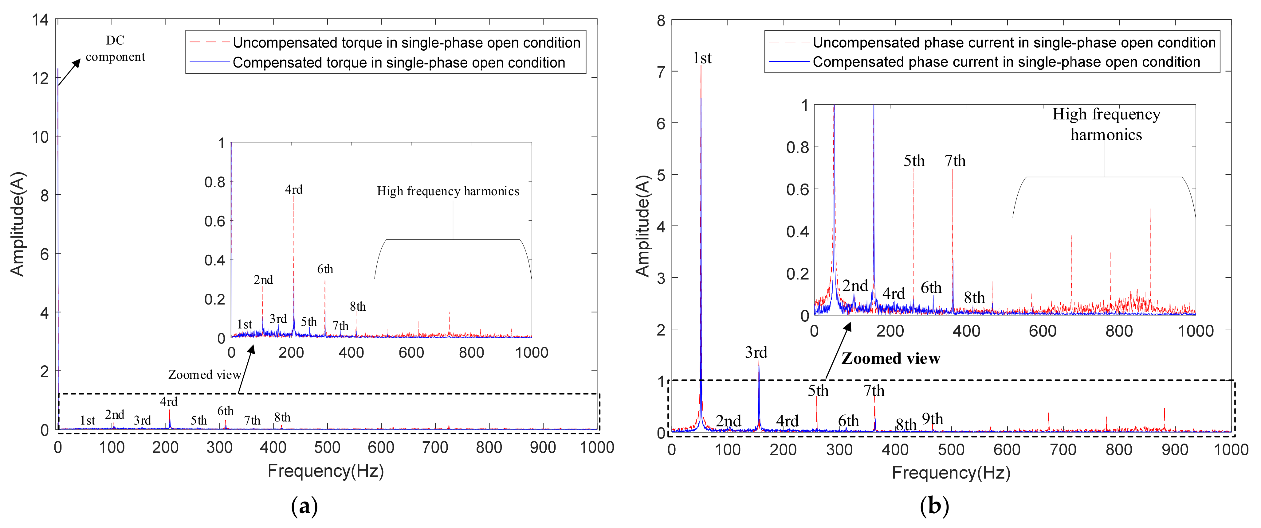
  • Under small third harmonic flux
    Figure 12a,b present the simulation test results of the machine side, DC bus voltage and grid side when Φ1 is 30 times more than Φ3 under operation at 0.393 MW. The fundamental frequency of the grid side is 50 Hz. With appropriate initializations, the whole system can reach the controlled mode at 0.04 s. At 0.06 s, phase “a” is set as an open circuit. At 0.1 s, the mSOGIs-based compensator for vpq* is activated. The other compensator for vsq* is then introduced after 0.05 s. From the first and second subplots in Figure 12a, it is clear that the speed fluctuations and torque ripples are suppressed via the compensators. The compensator for vsq* is used to constraint the harmonic disturbances in the secondary sub-generator, which is helpful in strengthening the fault tolerance combining with the compensator for the principal sub-generator. In the process of compensations, the perturbated degree of the control commands vpq* and vsq* are also reduced, according to the last subplot in Figure 12a, so as to directly reconfigure the PWM drive signals for the machine-side converter. However, the voltage command vsq* in the last subplot in the Figure 12a is much lower than vpq* in healthy conditions, while the fluctuation of vsq* is greater than vpq* once the single phase is open. Too great compensation for vsq* will worsen the suppression behaviors against the fluctuations, which will result in more perturbations in other control loops under the dual-loop control framework, such as the unconsidered d-axis control loops. That is to say, perturbations can “transfer” into other control loops. Consequently, the compensation gains are finally set as Kh_pq = 1 and Kh_sq = 0.1.
    In DC bus and grid side, as Figure 12b, the DC voltage, phase current as well as the output power of the grid-side converter (GSC) also perform attenuations of fluctuations under the single-phase open condition as the compensators are put into use. In detail, the power conversion processes create delays in the starting stage through the MSC and GSC. In steady states under healthy conditions, the powers in machine side, DC bus and grid side are almost equal. With compensations in faulty conditions, it is obvious that the fluctuations of power are also constrained. This is beneficial from the adopted fault-tolerant compensators in machine side. As a result, the proposed mSOGIs-based compensators are able to maintain the performance of the whole back-to-back conversion chain.
    Figure 12. Simulation result of compensation in q-axis current control loops when Φ13 = 30: (a) machine-side waveforms; (b) DC bus voltage and grid-side waveforms.
    Figure 12. Simulation result of compensation in q-axis current control loops when Φ13 = 30: (a) machine-side waveforms; (b) DC bus voltage and grid-side waveforms.
    Jmse 09 00574 g012
  • Under significant third harmonic flux
    In Figure 13, the magnet flux Φ1 is nine times of Φ3, which means that the third harmonic component in the back-EMFs is more significant in both healthy and faulty conditions. Fluctuations in machine side and grid side are well compensated, and their performance analysis is consistent with Figure 12. The only difference is that the gain of compensator Kh_sq for vsq* should be increased to adapt to the greater disturbances in the more important secondary sub-generator, and avoid injecting external interferences from the compensators. Thus, the compensation gains Kh_pq and Kh_sq are set as 1 and 0.35 m respectively.
    It should be noted that the test results in Figure 13, under a significant third harmonic flux, are independent to the MPPT characteristics. The nominal Φ3 related to the characteristics in Figure 3 is equal to 0.082 Wb. That is, Figure 12 shows a working point with νtides = 2.055 m/s in the MPPT characteristics. Figure 13 is performed to test the fault-tolerant control behaviors of the proposed FTC method under a condition of a greater trapezoidal deformation for the back-EMFs by increasing the flux parameter Φ3 in the numerical model and control strategy. The simulation results show that the proposed method can adapt well to the five-phase PMSG with different trapezoidal back-EMFs.

5. Experimental Verifications

In order to investigate the fault tolerance of the conversion chain under practical conditions, a small power-scale laboratory prototype in machine side was established, as Figure 14. This platform integrated a five-phase PMSG with trapezoidal back-EMFs and a five-leg power converter. The whole system worked in a standalone mode which provides the power electricity to a passive load. The electrical angle came from a 12-bit absolute encoder that coupled in the bearing of a DC motor which directly drives the five-phase PMSG. To emulate the external input of the tidal current speed, this rotor and stator of DC motor were under regulated by adjustable voltage sources. The dSPACE (Paderborn, Germany) plant was adopted as a center control unit which can process the input and output information of the physical parts through the ControlDesk software. All the test results were recorded by a multi-channel oscilloscope (YokogawaDL-750). The main parameters of this laboratory prototype can be found in Table A2 in Appendix A.
In this platform, the actual characteristics shown in Section 2.1 can be achieved by setting the equivalent ratio of the gearbox as 1:40 to synchronize the angular velocities, relative to the real turbine in the simulation. In practice, a tidal current turbine usually establishes a large moment of inertia with low-speed operations in order to obtain a large amount of kinetic energy from the sea water. In a short and limited period, the tidal current speed can be regarded as a constant profile (e.g., within one hour) for the simulation tests. Thus, the following tests are conducted under a constant tidal current speed. Moreover, the electromagnetic torque is calculated according to Equation (27).
In order to evaluate torque ripples and the total harmonic distortion (THD) of phase current, except the opened phase, two performance indicators are given as Equations (29) and (30).
THD = x = a , b , c , d , e THD i x 2 5 , where   THD i x = H = 2 n H i x _ H R M S 2 i x _ F u n d a m e n t a l R M S
Torque   ripple = max ( T e m ) min ( T e m ) / average ( T e m )
where the notation “average( )” presents an operation of mean values in continuous time operations. For ease of descriptions, hereafter “torque” specifically represents the electromagnetic torque. i x _ H R M S means the root mean square (RMS) value of the Hth harmonic component of the current in phase “x”. i x _ F u n d a m e n t a l R M S is the RMS value in terms of the fundamental frequency. H represents the harmonic order for calculating the THD. In this paper, the number of harmonics for the THD is set as nH = 15.

5.1. Harmonic Compensation Behaviors in Healthy Conditions

In healthy conditions, the mentioned system under control conventionally suffers from some unmodeled items, such as misalignment of the shaft, air-gap eccentricity, variations of corresponding parameters between control strategies and physical objects, measurement noises, etc. Regarding these unconsidered disturbances, an experimental test is implemented in healthy conditions as shown in Figure 15a,b. Here, current in phase “a” is used for the harmonic analysis.
In order to test the effectiveness of harmonic suppression in healthy conditions, the 1st, 3rd, 4th, 5th and 6th harmonics in Park’s frames are considered based on spectrum analysis of the waveforms. In Figure 15a, the distorted degree of phase current working around 50 Hz is improved significantly once the multiple SOGIs-based compensators are put into use. As shown in the bottom two zoomed subfigures in Figure 15b, the first 7 harmonics, except the necessary 1st and 3rd ones, are constrained in a satisfactory level, especially the 5th and 7th ones. The established multiple SOGIs-based compensators are also able to filter higher-order harmonics. This expected phenomenon is beneficial for the attenuation of high frequencies according to the bandpass characteristics, which is analyzed in Figure 7a. That is to say, the units of multiple SOGIs-based compensators can suppress the specific harmonics as well as with good filtering performance, which brings a reduction of THD from 43.23% to 32.84% through Equation (29). It should be pointed out that the channel of torque waveform is set as the “Analog current (AC)” mode hereafter to observe the torque ripples better. The detailed information of each channel can be found in the footnotes. Relying on Equation (30), the torque ripples are suppressed from 28.41% to 23.68% due to the compensators. This scenario shows that multiple SOGIs-based compensators have positive effects on the machinery system with better operation.
Figure 15. Test results and their harmonic spectra in healthy conditions: (a) experimental waveforms; (b) comparison of phase current spectra (e.g., in phase “a”).
Jmse 09 00574 g015

5.2. Fault Tolerance in Single-Phase Open Conditions

The previous subsection extends the generalization and usability of the proposed FTC strategy. This method mainly aims to improve the fault-tolerant performance of the system. This section mainly concentrates on the performance of the fault tolerance and the mechanism investigation of the proposed FTC strategy. Hence, the test results are given by setting an open circuit of phase “a”, illustrated as Figure 16a,b. Compared with the uncompensated situation in Figure 15a, the studied five-phase PMSG system will have nearly 1.4 times the peak values of the phase current shown in Figure 16a once a phase is open. Relative to the opened phase, there will be greater fluctuations in the adjacent phases (phase “b” and phase “e”) due to direct interactions among the phases. Consequently, torque ripples will increase by approximately 14.55% relative to the ones in healthy conditions and reach 42.96% and oscillate with a range of 4.05 nm. The power quality level of the phase current also degrades, containing the THD with 67.28% due to the phase loss. As mentioned before, the 2nd, 4th, 6th, 8th and 10th harmonic disturbances are estimated in real time from the ipq and isq control loops by the multiple SOGIs-based compensators, which reduce the torque ripples as well as enhance the power quality of the current. In detail, the torque ripples can be constrained into 29.54% with an approximately 31.2% reduction. The suppressed fluctuations settle during 2.23 nm according to the right-most zoomed illustration in Figure 16b. Under this condition, the THD calculated by Equation (30) of phase current becomes 41.74%.
To fully understand the operational mechanism of the multiple SOGIs-based compensators, spectra of phase torque and phase current (here phase-“b” current is adopted) are respectively presented as Figure 17a,b. Firstly, the torque contains even order harmonic disturbances, where the 2nd, 4th, 6th, 8th and 10th components become significant (marked with a zoomed view as Figure 17a, which is modeled by Equation (21) and deduced in Appendix B. The 8th and 10th harmonic disturbances are also considered in the mSOGIs as the phase current contains not only 1st and 3rd harmonic components with a phase-loss but also higher odd order harmonic disturbances, such as the 5th and 7th. These two additional harmonics will further inject nonnegligible 8- and 10-times harmonics into the ipq and isq current control loops, respectively.
In practice, the 10 times harmonic disturbances pollute all the control loops under the feedback frameworks of dual loops, which does not only affect the secondary sub-generator, as in the description in Table 2. As such, the 2nd, 4th, 6th, 8th, 10th harmonics are estimated and injected both to ipq and isq current control loops. Obviously, as depicted by the blue curve in Figure 17a, these additional interferences can be suppressed to satisfactory levels. Specially, it can be observed that the torque will contain negligible odd-order harmonics when the even ones are under-constrained, which are introduced due to the efficiency of harmonic estimation by the mSOGIs under the real-time variations of the mechanical speed that is used for harmonic resonances. Nevertheless, the compensated process guarantees the effective suppression of predominant harmonic disturbances, which inversely enhances the fault-tolerant availability of the system under the open circuit fault. Regarding the DC component in torque, the compensators maintain the level of torque since the multiple SOGIs can separate it out in real-time.
Figure 17. Harmonic analysis of torque and phase current: (a) spectra of electromagnetic torque; (b) spectra of phase current (e.g., in phase “b”).
Jmse 09 00574 g017
Accordingly, in Figure 17b, it is obvious to see the phase current contains additional odd order harmonics apart from the necessary 1st and 3rd harmonics, especially the 5th and 7th components. These two harmonics dominate the additional disturbances, which can be effectively suppressed by the multiple SOGIs-based compensators as the blue curve. It should be noted that the 6th harmonic component increases, and the harmonic disturbances are not constrained into zeros, which comes from the additional 5th and 7th harmonics that are unsuppressed in torque ripples under Park’s frames. In fact, this incomplete compensation is attributed to the lack of consideration for compensation in the d-axis and speed control loops. However, concerning compensations in more control loops could introduce heavier tasks of computational consumptions. This issue is ignored here, considering the suppression behaviors for the predominant 5th and 7th harmonics. In the same way as the healthy conditions in Figure 15, the high frequency interferences can also be filtered at the same time with these compensators. Table 3 shows that the copper losses have been effectively reduced using the multiple SOGIs-based compensators either in healthy or the single-phase open conditions. The copper losses are calculated based on Equation (16) with an average level within a same period of time, whose percentages, relative to the electromagnetic power (Temωm), are also presented in Table 3. The copper losses will be significant as one phase is open without any actions, which is mainly due to oversized current distortions and high-order harmonic interferences, as depicted in Figure 15a and Figure 16a, respectively. The proposed method has good filtering performance and fault tolerance, resulting in almost half the energy savings from the copper losses. Performance indicators are organized and analyzed, as shown in Table 3, according to the test results. With the analyzed performance of torque ripples and THD, in consequence, the proposed method presents satisfactory performance both in the healthy and faulty conditions.

6. Conclusions

A conveniently implemented model-free FTC strategy is proposed in this paper based on multiple SOGIs, applying to five-phase PMSG-based tidal current energy conversion systems. The harmonic disturbances (especially caused by 1st, 3rd, 5th, 7th harmonic components) are modeled firstly in an event of single-phase open circuit fault in the five-phase PMSG with trapezoidal back-EMFs. With reference to the prior harmonic analysis, even order additional harmonics from torque ripples are targeted to be suppressed and compensated. For this purpose, the dominant harmonic disturbances in different orders are accurately estimated using multiple SOGIs. These extracted harmonic disturbances are injected to the q-axis current control loops in order to constrain torque ripples and improve the fault tolerance of the entire system.
By using a real power-scale simulation setup, test results firstly show the advantages of five-phase PMSG over the classical three-phase one. The simulation setup validates that the proposed method can adapt well to different trapezoidal five-phase PMSGs, with the third harmonic component either being important or not. In addition, the disturbances of the full-power conversion chain are suppressed, which offers better post-fault operational performance during the tidal current energy harnessing process. To fully understand the operational mechanism of the proposed FTC method, experimental validations are carried out under a small-scale laboratory prototype emulating a tidal application. The test results show that the proposed method has suitable behaviors for harmonic disturbance suppression, both in healthy and single-phase open operation modes. The high-order harmonics can be also constrained with the filtering merits implicitly contained in the multiple SOGIs. When a single-phase is open, the compensation mechanism of the proposed method can help reduce almost half the copper losses and 31% torque ripples, maintaining the high availability in the post-fault operations.
This compensation mechanism via multiple SOGIs shows potentials to be extended to other kinds of related fault-tolerant issues and assisting classical PI controllers adapt to larger operational ranges. Due to these benefits, this proposed model-free FTC strategy (need only harmonic analysis) is a promising way to enhance the reliability and availability of practical tidal current applications in complicated under-sea environments.

Author Contributions

Z.L. established the simulation setup and laboratory prototype, implemented verifications of the proposed method and wrote this paper; A.H. helped in the realization and modifications to this paper; M.F.B. and M.M. modified the paper and evaluated the feasibility; T.T. offered directions on this paper. All authors have read and agreed to the published version of the manuscript.

Funding

This research was funded by the China Scholarship Council, Grant No. 201808310083 and AAP-WISE International.

Institutional Review Board Statement

Not applicable since this study did not involve humans or animals.

Informed Consent Statement

Not applicable.

Data Availability Statement

The data are available from the corresponding author upon reasonable request.

Acknowledgments

We would like to thank the funding and the laboratory prototype from IREENA laboratory.

Conflicts of Interest

The authors declare no conflict of interest.

Appendix A

Park transformation matrix TPark13 for trapezoidal back-EMFs (contains the 1st and 3rd). Note that in the equations in Appendix A and Appendix B, mechanical angular velocity is uniformly presented as Ω:
2 5 cos p Ω t cos p Ω t 2 π 5 cos p Ω t 4 π 5 cos p Ω t 6 π 5 cos p Ω t 8 π 5 sin p Ω t sin p Ω t 2 π 5 sin p Ω t 4 π 5 sin p Ω t 6 π 5 sin p Ω t 8 π 5 cos 3 p Ω t cos 3 p Ω t 6 π 5 cos 3 p Ω t 2 π 5 cos ( 3 p Ω t 8 π 5 ) cos ( 3 p Ω t 4 π 5 ) sin 3 p Ω t sin 3 p Ω t 6 π 5 sin 3 p Ω t 2 π 5 sin 3 p Ω t 8 π 5 sin 3 p Ω t 4 π 5 1 / 2 1 / 2 1 / 2 1 / 2 1 / 2
Park transformation matrix TPark1 for sinusoidal back-EMFs (contains only the 1st):
2 5 cos p Ω t cos p Ω t 2 π 5 cos p Ω t 4 π 5 cos p Ω t 6 π 5 cos p Ω t 8 π 5 sin p Ω t sin p Ω t 2 π 5 sin p Ω t 4 π 5 sin p Ω t 6 π 5 sin p Ω t 8 π 5 cos 0 cos 6 π 5 cos 2 π 5 cos ( 8 π 5 ) cos ( 4 π 5 ) sin 0   sin 6 π 5   sin 2 π 5   sin 8 π 5   sin 4 π 5 1 / 2 1 / 2 1 / 2 1 / 2 1 / 2
Table A1. Parameters of the real power-scale simulation setup.
SymbolDescriptionValue
JturInertia of turbine1.3131 × 106 kg∙m2
Pm_ratedGenerator rated power (at 50 Hz)1.5 MW
VdcDC-bus rated voltage 1700 V
ωm_ratedRotor-rated angular velocity (at 50 Hz)2.618 rad/s
nppPole pair number 120
Φ1Magnet flux in principle sub-generator2.458 Wb
Φ3Magnet flux in secondary sub-generator0.2731 Wb or 0.082 Wb
RsGenerator stator resistance 0.0081 Ω
LprPrinciple sub-generator inductances1.2 mH
LseSecondary sub-generator inductances0.88 mH
CdcDC-bus capacitor 13 mF
RfGrid-side resistance 0.1 mΩ
LfGrid-side inductance 1.5 mH
Table A2. Parameters of the small-scale laboratory prototype.
SymbolDescriptionValue
PnorminalNominal power of generator (at 110 Hz)3.3 kW
BM_dcFriction coefficient of DC motor’s shaft0.091
BgenFriction coefficient of generator’s shaft0.123
JM_dcInertia of DC motor0.02 kg·m2
JgenInertia of generator0.00137 kg·m2
ωm_norminalNominal angular velocity of generator230.3835 rad/s
pNumber of pole pairs3
Φ1, Φ3Magnet fluxes0.150 Wb, 0.0149 Wb
RsStator resistance0.540 Ω
LoadResistive load242 Ω
Lpr, LseEquivalent inductance5.1 mH, 3.2 mH
TpwmSwitching period0.1 ms
Kh_pq, Kh_sqCompensation gains0.55

Appendix B

Affected by 1st and 3rd current harmonics in original abcde frame under the single-phase open condition, the Equation (21) can be deduced as:
2 T e m * 5 p 1 + X r 2 Φ 1 2 5 i p d t = x 1 = b , c , d , e k = 1 , 2 , 3 , 4 η x 1 2 sin 2 p Ω t 2 k π 5 + θ x 1 + sin θ x 1 + x 3 = b , c , d , e k = 1 , 2 , 3 , 4 η x 3 2 sin 4 p Ω t 2 k π 5 + θ x 3 + sin 2 p Ω t 2 k π 5 + θ x 3 x 1 = b , c , d , e k = 1 , 2 , 3 , 4 η x 1 2 cos 2 p Ω t 2 k π 5 + θ x 1 cos θ x 1 + x 3 = b , c , d , e k = 1 , 2 , 3 , 4 η x 3 2 sin 4 p Ω t 2 k π 5 sin θ x 3 cos 2 p Ω t 2 k π 5 + θ x 3 x 1 = b , c , d , e k = 1 , 2 , 3 , 4 η x 1 2 sin 4 p Ω t 2 k π 5 + θ x 1 + sin 2 p Ω t 2 k π 5 θ x 1 + x 3 = b , c , d , e k = 1 , 2 , 3 , 4 η x 3 2 sin 6 p Ω t 2 k π 5 + θ x 3 + sin θ x 3 x 1 = b , c , d , e k = 1 , 2 , 3 , 4 η x 1 2 cos 4 p Ω t 2 k π 5 + θ x 1 cos 2 p Ω t 2 k π 5 + θ x 1 + x 3 = b , c , d , e k = 1 , 2 , 3 , 4 η x 3 2 cos 6 p Ω t 2 k π 5 + θ x 3 cos θ x 3 x 1 = b , c , d , e k = 1 , 2 , 3 , 4 2 η x 1 2 sin p Ω t 2 k π 5 + θ x 1 + x 3 = b , c , d , e k = 1 , 2 , 3 , 4 2 η x 3 2 sin 3 p Ω t 2 k π 5 + θ x 3
Similarly, the harmonic disturbances in Parks’ frames in Equation (21) are deduced as below due to the influences of the 5th and 7th additional harmonics components of the phase current under the original abcde frame.
2 T e m * 5 p 1 + X r 2 Φ 1 2 5 x 5 = b , c , d , e k = 1 , 2 , 3 , 4 η x 5 2 sin 6 p Ω t k π 5 + θ x 5 + sin 4 p Ω t k π 5 + θ x 5 + x 7 = b , c , d , e k = 1 , 2 , 3 , 4 η x 7 2 sin 8 p Ω t k π 5 + θ x 7 + sin 6 p Ω t k π 5 + θ x 7 x 5 = b , c , d , e k = 1 , 2 , 3 , 4 η x 5 2 cos 6 p Ω t k π 5 + θ x 5 cos 4 p Ω t k π 5 + θ x 5 + x 7 = b , c , d , e k = 1 , 2 , 3 , 4 η x 7 2 cos 8 p Ω t k π 5 + θ x 7 cos 6 p Ω t k π 5 + θ x 7 x 5 = b , c , d , e k = 1 , 2 , 3 , 4 η x 5 2 sin 8 p Ω t k π 5 + θ x 5 + sin 2 p Ω t k π 5 + θ x 5 + x 7 = b , c , d , e k = 1 , 2 , 3 , 4 η x 7 2 sin 10 p Ω t k π 5 + θ x 7 + sin 4 p Ω t k π 5 + θ x 7 x 5 = b , c , d , e k = 1 , 2 , 3 , 4 η x 5 2 cos 8 p Ω t k π 5 + θ x 5 cos 2 p Ω t k π 5 + θ x 5 + x 7 = b , c , d , e k = 1 , 2 , 3 , 4 η x 7 2 cos 10 p Ω t k π 5 + θ x 7 cos 4 p Ω t k π 5 + θ x 7 x 5 = b , c , d , e k = 1 , 2 , 3 , 4 2 η x 5 2 sin 5 p Ω t k π 5 + θ b 5 + x 5 = b , c , d , e k = 1 , 2 , 3 , 4 2 η x 7 2 sin 7 p Ω t k π 5 + θ b 7
here k is equal to 1, 2, 3 and 4, respectively, corresponding to remaining healthy phases “b”, “c, “d” and “e”. Any symbol of subscript from x 1 , x 3 , x 5 and x 7 varies from “b”, “c”, “d” and “e”.

References

  1. Sala, G.; Mengoni, M.; Rizzoli, G.; Degano, M.; Zarri, L.; Tani, A. Impact of star connection layouts on the control of multiphase induction motor drives under open-phase fault. IEEE Trans. Ind. Electron. 2021, 36, 3717–3726. [Google Scholar]
  2. Huang, W.; Hua, W.; Chen, F.; Hu, M.; Zhu, J. Model predictive torque control with svm for five-phase pmsm under open-circuit fault condition. IEEE Trans. Power Electron. 2020, 35, 5531–5540. [Google Scholar] [CrossRef]
  3. Cervone, A.; Slunjski, M.; Levi, E.; Brando, G. Optimal third-harmonic current injection for asymmetrical multiphase permanent magnet synchronous machines. IEEE Trans. Ind. Electron. 2021, 68, 2772–2783. [Google Scholar] [CrossRef] [Green Version]
  4. Xiong, C.; Guan, T.; Zhou, P.; Xu, H. A fault-tolerant foc strategy for five-phase spmsm with minimum torque ripples in the full torque operation range under double-phase open-circuit fault. IEEE Trans. Ind. Electron. 2020, 67, 9059–9072. [Google Scholar] [CrossRef]
  5. Hang, J.; Wu, H.; Zhang, J.; Ding, S.; Huang, Y.; Hua, W. Cost functionbased open-phase fault diagnosis for pmsm drive system with model predictive current control. IEEE Trans. Power Electron. 2021, 36, 2574–2583. [Google Scholar] [CrossRef]
  6. Liu, Z.; Wang, X.; Wang, F.; Chen, Z. Fault-tolerant consensus control with control allocation in a leader-following multi-agent system. J. Frankl. Inst. J. Frankl. I. 2020, 357, 9614–9632. [Google Scholar] [CrossRef]
  7. Wang, X. Active fault tolerant control for unmanned underwater vehicle with sensor faults. IEEE Trans. Instrum. Meas. 2020, 69, 9485–9495. [Google Scholar] [CrossRef]
  8. Jainm, T.; Yamé, J.J.; Sauter, D. Active Fault-Tolerant Control Systems, 1st ed.; Springer: Berlin/Heidelberg, Germany, 2017; pp. 1–9. [Google Scholar]
  9. Lan, J.; Patton, R.J. Integrated design of fault-tolerant control for nonlinear systems based on fault estimation and t–s fuzzy modeling. IEEE Trans. Fuzzy Syst. 2017, 25, 1141–1154. [Google Scholar] [CrossRef]
  10. Liu, G.; Lin, Z.; Zhao, W.; Chen, Q.; Xu, G. Third harmonic current injection in fault-tolerant five-phase permanent-magnet motor drive. IEEE Trans. Power Electron. 2018, 33, 6970–6979. [Google Scholar] [CrossRef]
  11. Tian, B.; Sun, L.; Molinas, M.; An, Q.T. Repetitive control based phase voltage modulation amendment for foc-based five-phase pmsms under single-phase open fault. IEEE Trans. Ind. Electron. 2021, 68, 1949–1960. [Google Scholar] [CrossRef]
  12. Boem, F.; Gallo, A.J.; Raimondo, D.M.; Parisini, T. Distributed faulttolerant control of large-scale systems: An active fault diagnosis approach. IEEE Control Netw. Syst. 2020, 7, 288–301. [Google Scholar] [CrossRef] [Green Version]
  13. Zhang, H.; Han, J.; Luo, C.; Wang, Y. Fault-tolerant control of a nonlinear system based on generalized fuzzy hyperbolic model and adaptive disturbance observer. IEEE Trans. Syst. Man Cybern. Syst. 2017, 47, 2289–2300. [Google Scholar] [CrossRef]
  14. Liu, D.; Yang, Y.; Li, L.; Ding, S.X. Control performance-based faulttolerant control strategy for singular systems. IEEE Trans. Syst. Man Cybern. Syst. 2020, 50, 2398–2407. [Google Scholar] [CrossRef]
  15. Liu, Z.; Houari, A.; Machmoum, M.; Benkhoris, M.F.; Tang, T.H. An Active FTC Strategy Using Generalized Proportional Integral Observers Applied to Five-Phase PMSG based Tidal Current Energy Conversion Systems. Energies 2020, 13, 6645. [Google Scholar] [CrossRef]
  16. Kiselev, A.; Catuogno, G.R.; Kuznietsov, A.; Leidhold, R. Finitecontrol- set mpc for open-phase fault-tolerant control of pm synchronous motor drives. IEEE Trans. Ind. Electron. 2020, 67, 4444–4452. [Google Scholar] [CrossRef]
  17. Azizi, A.; Nourisola, H.; Shoja-Majidabad, S. Fault tolerant control of wind turbines with an adaptive output feedback sliding mode controller. Renew. Energy 2019, 135, 55–65. [Google Scholar] [CrossRef]
  18. Rodríguez, P.; Luna, A.; Candela, I.; Mujal, R.; Teodorescu, R.; Blaabjerg, F. Multiresonant frequency-locked loop for grid synchronization of power converters under distorted grid conditions. IEEE Trans. Ind. Electron. 2011, 58, 127–138. [Google Scholar] [CrossRef] [Green Version]
  19. Torres, L.; Jiménez-Cabas, J.; González, O.; Molina, L.; López-Estrada, F.-R. Kalman Filters for Leak Diagnosis in Pipelines: Brief History and Future Research. J. Mar. Sci. Eng. 2020, 8, 173. [Google Scholar] [CrossRef] [Green Version]
  20. Tian, G.; Zhou, Q.; Birari, R.; Qi, J.; Qu, Z. A hybrid-learning algorithm for online dynamic state estimation in multimachine power systems. IEEE Trans. Neural Netw. Learn. Syst. 2020, 31, 5497–5508. [Google Scholar] [CrossRef] [PubMed]
  21. Yang, H.; Jiang, Y.; Yin, S. Fault-tolerant control of time-delay markov jump systems with itô stochastic process and output disturbance based on sliding mode observer. IEEE Trans. Ind. Informat. 2018, 14, 5299–5307. [Google Scholar] [CrossRef]
  22. Liu, W.; Li, P. Disturbance observer-based fault-tolerant adaptive control for nonlinearly parameterized systems. IEEE Trans. Ind. Electron. 2019, 66, 8681–8691. [Google Scholar] [CrossRef]
  23. Yao, X.; Wu, L.; Guo, L. Disturbance-observer-based fault tolerant control of high-speed trains: A markovian jump system model approach. IEEE Trans. Syst. Man Cybern. Syst. 2020, 50, 1476–1485. [Google Scholar] [CrossRef]
  24. Gou, B.; Ge, X.L.; Pu, J.K.; Feng, X.Y. A fault diagnosis and fault tolerant control method for DC-link circuit using notch filter in power traction converter. In Proceedings of the 2016 IEEE 8th International Power Electronics and Motion Control Conference (IPEMC-ECCE Asia), Hefei, China, 22–26 May 2016; pp. 3230–3235. [Google Scholar]
  25. Hu, P.F.; He, Z.X.; Li, S.Q.; Guerrero, J.M. Non-ideal proportional resonant control for modular multilevel converters under sub-module fault conditions. IEEE Trans. Energy Convers. 2019, 34, 1741–1750. [Google Scholar] [CrossRef]
  26. Lewis, M.; O’Hara Murray, R.; Fredriksson, S.; Maskell, J.; Fockert, A.D.; Neill, S.P.; Robins, P.E. A standardised tidal-stream power curve, optimised for the global resource. Renew. Energy 2021, 170, 1308–1323. [Google Scholar] [CrossRef]
  27. Kolar, J.W.; Friedli, T.; Krismer, F.; Looser, A.; Schweizer, M.; Friedemann, R.A.; Steimer, P.K.; Bevirt, J.B. Conceptualization and multiobjective optimization of the electric system of an airborne wind turbine. IEEE Trans. Emerg. Sel. Top. Power Electron. 2013, 1, 73–103. [Google Scholar] [CrossRef]
  28. Liu, Z.; Houari, A.; Machmoum, M.; Benkhoris, M.F.; Tang, T. A second order filter-based fault detection method for five-phase permanent magnet synchronous generators. In Proceedings of the 46th Annual Conference of the IEEE Industrial Electronics Society, Singapore, 18–21 October 2020; pp. 4827–4832. [Google Scholar]
  29. Kestelyn, X.; Semail, E. A vectorial approach for generation of optimal current references for multiphase permanent-magnet synchronous machines in real time. IEEE Trans. Ind. Electron. 2011, 58, 5057–5065. [Google Scholar] [CrossRef] [Green Version]
  30. Hwang, J.; Wei, H. The current harmonics elimination control strategy for six-leg three-phase permanent magnet synchronous motor drives. IEEE Trans. Power Electron. 2014, 29, 3032–3040. [Google Scholar] [CrossRef]
  31. Xiao, F.; Dong, L.; Li, L.; Liao, X. A frequency-fixed sogi-based pll for single-phase grid-connected converters. IEEE Trans. Power Electron. 2017, 32, 1713–1719. [Google Scholar] [CrossRef]
  32. Pham, H.; Bourgeot, J.; Benbouzid, M. Fault-tolerant finite control set-model predictive control for marine current turbine applications. IET Renew. Power Gener. 2018, 12, 415–421. [Google Scholar] [CrossRef]
  33. Mekri, F.; Elghali, S.B.; Benbouzid, M.E.H. Fault-Tolerant Control Performance Comparison of Three- and Five-Phase PMSG for Marine Current Turbine Applications. IEEE Trans. Sustain. Energy 2013, 4, 425–433. [Google Scholar] [CrossRef]
Figure 1. Configurations of back-to-back tidal current energy conversion systems integrated five-phase PMSG: (a) machine and grid side are installed offshore and transmission via submarine cables; (b) machine side in offshore and transmission via submarine cables to onshore grid side; (c) five-phase PMSG is installed offshore, transmission via submarine cables to onshore machine side converter (MSC) and onshore grid side.
Jmse 09 00574 g001
Figure 4. Structures of drive train models: (a) type with gearbox in small power-scale laboratory prototype (Ngear > 1); (b) gearless type in real power-scale simulation setup (Ngear = 1).
Jmse 09 00574 g004
Figure 5. Transformations of principal and secondary generators: (a) in principal sub-space; (b) in secondary sub-space.
Jmse 09 00574 g005
Figure 6. Block diagram of single SOGI in continuous time domain.
Jmse 09 00574 g006
Figure 7. Bode plots of transfer functions of a SOGI with various ωsogi: (a) Fα(s), Ks= 2 ; (b) Fβ(s), Ks= 2 .
Jmse 09 00574 g007
Figure 8. Description of multiple SOGIs and bode plot comparisons with different structures of SOGIs: (a) structure of multiple SOGIs; (b) bode plots of different design of SOGIs (e.g., extract 1st harmonic).
Jmse 09 00574 g008
Figure 10. Simulation schematic of a 1.5 MW five-phase PMSG-based TCECS.
Jmse 09 00574 g010
Figure 11. Comparison results of three- and five-phase PMSG-based systems: (a) mechanical angular velocities; (b) electromagnetic torques and mechanical torque; (c) phase current of three-phase PMSG-based system; (d) phase current of five-phase PMSG-based system; (e) powers of three-phase PMSG-based system; (f) powers of five-phase PMSG-based system.
Jmse 09 00574 g011
Figure 13. Simulation result of compensation in q-axis current control loops when Φ13 = 9: (a) machine-side waveforms; (b) DC bus voltage and grid-side waveforms.
Jmse 09 00574 g013
Figure 14. Small power-scale laboratory prototype emulating a machine-side tidal application.
Jmse 09 00574 g014
Figure 16. Test results and their harmonic spectra in healthy conditions by introducing the compensations: (a) without compensations as phase “a” is open; (b) with compensations as phase “a” is open.
Jmse 09 00574 g016
Table 1. Parameters of power coefficient function Cp.
SymbolValueSymbolValue
C10.6406C410.778
C2116.664C516
C30.4C60.0053
Table 2. General description of harmonic distribution of current/back-EMFs under healthy and single-phase open conditions.
Conditions
HealthySingle-Phase Open (e.g., Phase “a” Is Open)
Frames
Original Framephase ‘aMainly contains 1st and 3rd harmonics
(Others are regarded as disturbances)
Almost equal to 0
phase ‘bMainly contains 1st, 3rd, 5th and 7th harmonics
phase ‘c
phase ‘d
phase ‘e
Park’s Framepd axisAlmost equal to 0Mainly contains 2nd, 4th, 6th, 8th harmonics
pq axisAlmost an offset DC component
sd axisAlmost equal to 0Mainly contains 2nd, 4th, 6th, 8th and 10th harmonics
sq axisAlmost an offset DC component
HomopolarAlmost equal to 0Mainly contains 1st, 3rd, 5th and 7th harmonics
Table 3. Performance indicators in different working conditions.
IndicatorsCopper Losses (W)Torque Ripples (%)THD (%)
Working Conditions
HealthyNo compensations46.65 (3.40% loss)28.4143.23
By compensations40.41 (2.99% loss)23.6832.84
Single-Phase Open No compensations69.93 (5.32% loss)42.9667.28
By compensations34.24 (2.56% loss)29.5441.74
Publisher’s Note: MDPI stays neutral with regard to jurisdictional claims in published maps and institutional affiliations.

