Abstract
Environmental conditions in Arctic waters pose challenges to various offshore industrial activities. In this regard, better prediction of meteorological and oceanographic conditions contributes to addressing the challenges by developing economic plans and adopting safe strategies. This study revolved around simulation of meteorological and oceanographic conditions. To this aim, the applications of Bayesian inference, as well as Monte Carlo simulation (MCS) methods including sequential importance sampling (SIS) and Markov Chain Monte Carlo (MCMC) were studied. Three-hourly reanalysis data from the NOrwegian ReAnalysis 10 km (NORA10) for 33 years were used to evaluate the performance of the suggested simulation approaches. The data corresponding to the first 32 years were used to predict the meteorological and oceanographic conditions, and the data corresponding to the following year were used to model verification on a daily basis. The predicted meteorological and oceanographic conditions were then considered as inputs for the newly introduced icing model, namely Marine-Icing model for the Norwegian Coast Guard (MINCOG), to estimate sea spray icing in some regions of the Arctic Ocean, particularly in the sea area between Northern Norway and Svalbard archipelago. The results indicate that the monthly average absolute deviation (AAD) from reanalysis values for the MINCOG estimations with Bayesian, SIS, and MCMC inputs is not greater than 0.13, 0.22, and 0.41 cm/h, respectively.
1. Introduction
As a matter of global warming and ice melting in the Arctic, more waters are being opened and consequently, the marine traffic for both industrial and leisure purposes has largely been increasing. The Arctic regions encompass potential resources of oil and gas condensate, natural gas, diamond, timber, non-ferrous and rare metals, gold, and platinum. China and Japan have recently shown an increased interest in the development of transportation in the Northern Sea Route (NSR) since it is almost two times shorter than other sea routes from Europe to the Far East. During the past two decades, the flow of tourists to the Arctic has increased by more than 18 times, exceeding the population of Inuit and Danes, the indigenous residents of the area [1].
However, neglecting the predictions of the environmental hazardous condition, such as sea spray icing, in preparing plans for offshore industrial activities and sea voyages in the Arctic might cause long delays, extra expenses, additional energy consumption and CO2 emission, serious injuries, and fatalities. Icing may impact offshore operations, reduce safety, operational tempo and productivity, cause malfunction of the operational and communication equipment, slippery handrails, ladders or decks, unusable fire and rescue equipment, and the blocking of air vents [2,3]. The icing on vessels may also lead to severe accidents and capsizing [4,5]. Ice accumulation also influences the operability of vessels as well as offshore production structures and facilities by increasing power losses, failure rate, and frequency of need for inspection and repair. Additionally, it reduces the useful lifetime of the equipment and imposes safety hazards [6]. Furthermore, ice accretion on vessels can significantly increase the load as well as the energy that is required for de-icing purposes. Consequently, the fuel consumption will be raised that leads to additional CO2 emissions.
Wide varieties of anti-icing and de-icing techniques and technologies are available to enhance icing safety and protection such as chemicals, coatings, heat, and high-velocity fluids, air, and steam [7]. Moreover, forecasting the amount and the frequency of ice formation aids the selection of safety-enhancing strategies and ice protection technologies. Forecasting, also, can aid in tactical preparation before an icing event [2]. Nevertheless, forecasting icing events and rate is a complicated task due to the chaotic nature of icing and its correlation with a large number of parameters. Extensive works have been conducted on historical icing data to predict icing events [8]. Accordingly, the data have been examined from different perspectives such as the influence of meteorological and oceanographic conditions on icing rate from the statistical point of view [9], and introducing sea spray algorithms based on the collision of ship and waves considering the environmental data as input parameters [8,10]. The history and development of sea spray icing predictive models have been reviewed in [3,11].
Icing is mainly from two sources including sea spray caused by the collision of the ship and waves, and atmospheric icing caused by fog, Arctic sea smoke, high-velocity wind, and rain/drizzle or snow [7]. Sea spray is generated during the collision of vessel and waves, and by strong winds ripping off small droplets from the crest of breaking waves. However, the amount of water generated by wind is much smaller compared to sea spray generated during the collision of vessel and waves. The collision of waves and vessels leads to the formation of a spray-cloud, which its droplets will be transported by air and settled onto different surfaces of the vessel. In this regard, waves, vessel, seawater, and air contribute to ice generation. Accordingly, the characteristic of each factor such as height and period of the wave, speed and direction of the vessel, the salinity of seawater, wind speed, temperature, relative humidity, and pressure of air are influential [8,12].
ICEMOD [13,14] and RIGICE04 [15] are two commonly used simulation models for estimating the icing rates on a vessel. However, the newly developed model, Marine-Icing model for the Norwegian Coast Guard (MINCOG), provides higher verification scores (i.e., lower errors from the observations) than previously applied vessel-icing models, particularly using the data obtained in the Norwegian Arctic waters [8,16]. The MINCOG model has been developed based on the modelling of sea spray from wave-vessel interaction, which is considered as the main water source in vessel-icing events [16].
To estimate the sea spray icing for the future, the required input parameters of the MINCOG model should be predicted and plugged into the model. This study proposes methods for long-term prediction of meteorological and oceanographic conditions including wave height, wind speed, temperature, relative humidity, atmospheric pressure, and wave period, which are used as inputs in the MINCOG model to simulate sea spray icing. More details about the MINCOG model can be found in [8]. The area of this study is the sea area between Northern Norway and Svalbard archipelago, bounded to the latitudes 69° N to 78° N and longitudes 8° E to 36° E. However, the methodologies can be applied for the simulation of meteorological and oceanographic conditions in other locations. In this regard, the applications of Bayesian inference, as well as Monte Carlo simulation (MCS) methods comprising sequential importance sampling (SIS) and Markov Chain Monte Carlo (MCMC) in the prediction of meteorological and oceanographic conditions are studied and relevant approaches are proposed. 3-hourly reanalysis data from NOrwegian ReAnalysis 10 km (NORA10) [17] for 33 years are used to evaluate the performance of the suggested simulation approaches. To this aim, the data corresponding to the first 32 years are used to predict the meteorological and oceanographic conditions. The data corresponding to the following year are then used to model verification on a daily basis.
2. Methods
In attempting to anticipate future patterns of meteorology and oceanography, the behavior of the system can be modelled based on the available information on the movements of different parameters among their possible states and their interactions, although no model can fit the reality in all details. A large amount of numerical data are produced by meteorological observation systems and computer models, whilst obtaining insights about batches of numbers is a critical task. To this aim, statistical inference draws conclusions about the characteristics of a “population” based on a data sample by extracting its underlying generating process. In this context, statisticians use the Bayesian inference, according to which a parametric distribution is assumed to characterize the nature of the data-generating process where the parameter (s) of the distribution is the subject of uncertainty. Accordingly, prior information about the parameter of interest is quantified by a probability distribution, which may or may not be of a familiar parametric form. This prior information is then modified by combining it with the information provided by the data sample, in an optimal way [18,19]. Consequently, Bayesian inference provides a proper understanding of the stochastic nature of the parameter. Therefore, and given the credibility and ease in the model development procedure, the Bayesian inference has been recognized as a promising analysis technique to tackle events with chaotic nature [20].
Alternatively, the MCS method is the other powerful modelling tool dealing with complex and chaotic events to achieve a closer adherence to reality. MCS is generally defined as a methodology to estimate the solution of mathematical problems using random numbers. Taking advantage of the present powerful computers, the MCS method is continuously improving and becoming more practicable in modelling complex systems and problems in a variety of scientific domains. SIS and MCMC are known as two strong MCS-based techniques based on which conditional samples are drawn according to a Markov chain [21,22]. These techniques are discussed in this study since they seem to be relevant to the purpose of the study which is the simulation of the future behavior of meteorological and oceanographic conditions given past evidence.
2.1. Bayesian Inference
As mentioned above, the Bayesian inference is a parametric view of probability in which the parameters of probability distributions are the subject of inference. A parametric distribution quantitatively characterizes the dependency of the nature of the data-generating process on the parameter about which inferences are being drawn. For instance, if the data have been achieved through n identical and independent Bernoulli trials, the binomial distribution can be considered the data-generating model and the binomial parameter, p, is the target of statistical inference, which can fully describe the nature of the data-generating process [19].
Regardless of the variable of interest is discrete or continuous the parameter that is the subject of inference is generally continuous and can be presented by a probability density function (PDF). Accordingly, Bayes’ theorem for continuous probability models can be represented as follows [19]:
where, is the parameter that is the subject of inference (e.g., p in the binomial distribution or in a Poisson distribution), and x are the data in hand. Subjective belief about the parameter is described by the prior distribution which is generally a PDF since is a continuous parameter. However, different forms of may be chosen by different analysts. Furthermore, the likelihood, , represents the general nature of the data-generating process, which will be influenced by different values of . It is worth mentioning that the likelihood is in fact a function of the parameter based on fixed values of x rather than a function of x based on fixed-parameter . In other words, expresses the relative plausibility of the data as a function of possible values of . Consequently, the posterior distribution,, results from updating the prior distribution considering the information provided by the likelihood, [19].
Gaining insight about unobserved data values in the future by quantifying the uncertainty of the parameter is the ultimate goal of the Bayesian inference. To this aim, a PDF, namely predictive distribution, is derived by combining the parametric data-generating process and the posterior distribution for , which is given by Equation (2) [19],
where x+ represents the unobserved data in the future and x denotes the data in hand which have already been used to derive the posterior distribution, . It should be noted that is the PDF for the data given a particular value of , not the likelihood for given a fixed data sample x, although the two have the same notation. The posterior PDF, , quantifies uncertainty regarding based on the most recent probability updates. Equation (2) is indeed a weighted average of the PDFs for all possible values of , where the posterior distribution provides the weights [19].
Gaussian Data-Generating Process
In this study, it is assumed that the generating process of the data is Gaussian with known variance since it is easier for analytic treatment using conjugate prior and posterior distributions. This assumption will later be examined through a test of hypothesis in the experiments. The procedure to cope with the case in which the distribution of parameters of the generating process (i.e., and ) are unknown is available in [23,24]. Considering this assumption, in the situation where the conjugate prior and posterior distributions are Gaussian is computationally convenient, although it is confusing in notation due to four sets of means and variances. Moreover, when the posterior is Gaussian, the predictive distribution will also be Gaussian [19]. Below is the notation of the sets of means and variances:
- : mean of the data-generating process;
- : known variance of the data-generating process;
- : hyper-parameters of Gaussian prior distribution;
- : sample mean;
- : hyper-parameters of Gaussian posterior distribution;
- : parameters of Gaussian predictive distribution.
The detailed mathematics and formulations are provided by Wilks (2011) and summarized in [25]. Accordingly, the posterior hyper-parameters are as follows [19]:
The posterior mean is indeed a weighted mean of prior and sample means with a relatively greater weight for the sample mean, which rises as the sample size increases. This property leads to less dependency of prediction on the old less reliable data and instead emphasizes recently sampled data. The variance of the posterior is also smaller than both the prior and the known data-generating variances and even decreases as the sample size increases. Another aspect regarding the posterior parameters is that since the variance of the data-generating process () is known, only the sample mean appears in the estimations and neither the sample variance nor the amount of additional data can enhance our knowledge about it.
The variability of the sampling, which is of a Gaussian data-generating process, combining with the uncertainty about which is expressed by posterior causes uncertainty about future values of x+. Considering these two contributions, the Gaussian predictive distribution parameters are as follows [19]:
2.2. Sequential Importance Sampling
MCS is commonly applied to estimating the value of complicated integrals. Accordingly, when the target density, , is too complex to calculate its definite integral, MCS estimates its value using another density, , so-called proposal density or envelope, which covers in its domain and is analytically easier to sample. A relatively more efficient form of the MCS method to approximate integrals is importance sampling (IS). Briefly, in the IS method, the drawn samples from the proposal density are weighted to correct the sampling probabilities so that the weights are related to the target density. The weighted sample is particularly useful to estimate expectations under . Let be any arbitrary function. The expected value of is then approximated as follows [26,27]:
where is drawn from , .
The weights can also be standardized so they sum to 1, although it is not necessary. Therefore, IS can be seen as an approximation of by a discrete distribution and weights as masses of observed points. Rubin [28,29] proposed sampling from this discrete distribution, which is called sampling importance resampling (SIR). Accordingly, as the number of samples increases, the distribution of the random draws converges to [27]. However, as the dimension of the target density raises, the efficiency of SIR declines and it can be difficult to implement. It is challenging to specifying a very good high-dimensional envelope that properly approximates with sufficiently heavy tails but little waste. This drawback is addressed by sequential Monte Carlo (SMC) methods according to which the high-dimensional task is split into a sequence of simpler steps, each of which updates the previous one [27].
Let denote a discrete-time stochastic process where is the state of the random variable at time and represents the entire history of the sequence thus far. For simplicity, the scalar notation is adopted here; however, may be multidimensional. Meanwhile, the density of is denoted as . Consider that at time the expected value of is supposed to be estimated with respect to and using an IS strategy. One strategy would be directly using the SIR approach to sample sequences from an envelope and then the expected value of can be estimated by calculating the importance weighted average of this sample. However, in this strategy, as is increasing, and the expected value of evolve. Therefore, at time it would be reasonable to update previous inferences rather than acting as if there is no previous information. An alternative strategy is to append the simulated to the that previously simulated. Consequently, to estimate the expected value of , the previous importance weights are to be adjusted. This approach is called SIS [27,30,31].
2.2.1. Sequential Importance Sampling for Markov Processes
Assuming is a Markov process, depends only on rather than the whole history . Accordingly, the target density can be expressed as follows [27,31]:
Similarly, by adopting the same Markov form for the envelope, we have [27,31]:
According to the ordinary non-sequential SIR, as a sample is drawn from at time , each is to be reweighted by , whilst, based on SIS in a Markov process, we have [27,31]:
where and for .
Having and in hand and using the Markov property, the next component, , can be sampled and appended to . Moreover, can be adjusted using the multiplicative factor . Accordingly, the SIS algorithm for a Markov process initializes by sampling from and lets . Thereafter, for the next component , it draws sample from and lets . Using a sample of such points and their weights, and thus the expected value of can be approximated. The algorithm is given in [27].
To obtain an independent sample of size from , the algorithm can be carried out considering the sequences one at a time or as a batch. Consequently, the estimation for the weighted average of the quantity of interest, , is as below [27]:
The standardization of the weights at the end of each cycle is not essential, while if the estimation of is of interest, the normalization is natural [27].
2.3. Markov Chain Monte Carlo
MCMC is considered to be the most common computational method for Bayesian analysis of complex models. Whereas IS generates independent draw and related weights, MCMC methods build a Markov chain, generating dependent draws that have stationary density. Although creating such a Markov chain is often easy, there is still a bit of art required to construct an efficient chain with reasonable convergence speed [26].
2.3.1. The Metropolis–Hastings Algorithm
A very general method to implement MCMC is the Metropolis–Hastings algorithm. Accordingly, given that we already have a sample from a target density , a new sample is drawn from a proposal density . Moreover, the new sample is accepted or rejected according to an acceptance probability, , which depends on the previous draw and is to be updated in each iteration (see Equation (12)). One of the key properties of this method is that the density of will also be . The algorithm obtains a sequence with the stationary density of [26,27]. The algorithm is given in [26].
2.3.2. Convergence Diagnostic
A critical issue in the implementation of MCMC simulation is the time before the chain settles down to a steady-state so-called “converged”. To mitigate the possibility of bias due to the effect of the starting values, the iterations within the initial transient phase are usually discarded. Rates of convergence on different target distributions vary considerably, which makes it difficult to determine the length of the required initial transient phase [32]. Many techniques have been developed trying to determine the convergence of a particular Markov chain as reviewed in [32]. However, it is not generally possible to estimate the Markov chain convergence rate and then determine sufficient iterations to satisfy a prescribed accuracy measure [33,34].
In this study, the variability of the estimations in the iterations is evaluated via the absolute form of coefficient of variation (CV) and considered as a useful measure of convergence. To this aim, the algorithm is firstly supposed to proceed with a certain amount of iterations and then continues as long as the last outcomes considerably vary [19,22]. Thus, the absolute value of CV for the last outcomes, , which is calculated below, should be larger than a threshold, denoted as .
where and indicate the standard deviation and the expected value of the sampled values, respectively.
2.4. Proposed Models
The aforementioned approaches cannot be directly used in their standard form and some modifications and assumptions are required. For instance, in the Bayesian approach, to consider the effect of climate change, the old less reliable data are used to estimate the prior distribution, which is then modified by the newer sets of data from recent years to estimate the posterior distribution. Moreover, the normal distribution function is used in the Bayesian approach to fit the data, whilst, in SIS and MCMC models, the data are fitted using kernel smoothing function, which is indeed the target density, and the Weibull distribution function is used as the proposal density.
It is worth mentioning here that the kernel density estimate is an extension of the histogram that does not require arbitrary rounding to bin centers, and provides a smooth result. Indeed, kernel density estimate is a nonparametric alternative to fit the common parametric PDFs. Further details in this regard are available in [19,27].
As mentioned before, the area of the study is the Arctic offshore, specifically, the sea area between Northern Norway and Svalbard archipelago bounded to the latitudes 69° N to 78° N and longitudes 8° E to 36° E (see Figure 1). The offshore location with coordinates (74.07° N, 35.81° E) is selected for analysis of the meteorological and oceanographic conditions and, icing events and rates since it is currently open for petroleum activity. These coordinates, as illustrated in Figure 1, are located approximately 500 km east of Bjørnøya in the Norwegian part of the Barents Sea, where the discovery wellbore 7435/12-1 was drilled in 2017 [35].
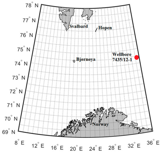
Figure 1.
The study area between Northern Norway and Svalbard archipelago bounded to the latitudes 69° N to 78° N and longitudes 8° E to 36° E.
In the following, after defining required assumptions, proposed models are developed by combining and modifying the above-mentioned approaches. Thereafter, using the data from 32 years (1980–2011), the six meteorological and oceanographic conditions, including wave height, wind speed, temperature, relative humidity, atmospheric pressure, and wave period, are simulated for one year on a daily basis and the results are compared with the 33rd year (2012). Then, the predicted values are used as input parameters in the MINCOG model to forecast the icing rate.
2.4.1. Proposed Bayesian Approach
After some investigations in developing a Bayesian framework, to mitigate the effect of climate change, the older data during 27 years from 1980 to 2006, are used to estimate the prior distribution, which is then modified by the newer sets of data, from 2007 to 2011, to estimate the posterior distribution. Accordingly, it is assumed that the prior data-generating process for the daily average of each meteorological and oceanographic condition is Gaussian over the years 1980 to 2006. It is worth mentioning here that the parameter of the Gaussian predictive distribution is then considered as an estimation for the meteorological and oceanographic condition. Meanwhile, the assumption is evaluated for the six meteorological and oceanographic conditions in coordinates (74.07° N, 35.81° E) using the Anderson–Darling test at the 5% significance level, where the null hypothesis (i.e., H0) is that the parameter is from a population with a normal distribution, against the alternative hypothesis (i.e., H1) that the parameter is not from a population with a normal distribution [36]. Accordingly, and based on the data over 27 years (1980–2006), the null hypothesis cannot be rejected in the majority of the days. The results of the Anderson–Darling test are shown in Table 1, where the number and percentage of the days that the null hypothesis cannot be rejected are mentioned. Likewise, the posterior data-generating process is assumed to be Gaussian with unknown parameters, and then the newer sets of data during five years (2007–2011) are considered as a sample to modify the prior distribution and determine the posterior distribution. However, the variance of the data-generating process, , is considered to be known and daily average values of meteorological and oceanographic conditions during 32 years (1980–2011) are used to calculate its value.

Table 1.
The Anderson–Darling test at the significance level of 5%, for normality test of the daily average of meteorological and oceanographic conditions in coordinates (74.07° N, 35.81° E).
2.4.2. Proposed Sequential Importance Sampling Algorithm
The drawback of the standard SIS that was defined in Section 2.2.1 is that the deviation of estimation at each state will be added to the deviation from the previous state so that the algorithm hardly converges to a value. Therefore, rather than sampling dependent draws from static densities, the target and proposal densities are defined in a way to be dependent on the previous state. To this aim, the deviation of each day from the previous day in 32 years (1980–2011) was extracted from the dataset. Therefore, the conditional density at each state is achieved by estimating the average of the previous state adding to the possible deviations. Accordingly, a kernel smoothing density with Gaussian kernel function is considered as the target density. Moreover, Weibull distribution is used as the proposal density. However, since the Weibull distribution is defined only for positive values, a data shifting procedure is embedded in the algorithm. Accordingly, a positive value, , is to be added to all the data, which is calculated via Equation (14).
where is the index of bins in the kernel density estimation and represents the center of the bin. It should be mentioned that ‘’ must be later subtracted from the simulated results. Furthermore, the parameters of the Weibull distribution are estimated by the maximum likelihood estimation (MLE) method considering 32 years of the data (1980–2011). Consequently, the algorithm iterates until a defined number of samples, , is drawn. Thus, the performance of the algorithm using two sizes of and , namely SIS200 and SIS500, are investigated. The proposed SIS algorithm for prediction of meteorological and oceanographic conditions is outlined in Algorithm 1.
| Algorithm 1 Proposed sequential importance sampling (SIS) for prediction of meteorological and oceanographic conditions. |
|
2.4.3. Proposed Markov Chain Monte Carlo Algorithm
To apply the MCMC approach, a modified Metropolis–Hastings algorithm is developed in which the IS concept is embedded. Similar to SIS, the kernel smoothing density and the Weibull distribution function are considered as the target and proposal density, respectively. Therefore, for parameters that might hire non-positive values such as temperature, the shifting procedure is also required. Furthermore, a dynamic stopping criterion is added to the algorithm based on which the algorithm iterates until the CV in the last iterations (see Equation (13)) drops below the CV threshold, , which implies the algorithm no longer achieves different results. Moreover, to avoid early stoppage, the stopping criterion is to be activated after a certain amount of iterations, , namely iteration lower bound. Thus, two sizes of and are later investigated which are called MCMC200 and MCMC500, respectively. Algorithm 2 indicates the steps of the proposed MCMC algorithm for prediction of meteorological and oceanographic conditions.
| Algorithm 2 Proposed Markov chain Monte Carlo (MCMC) for prediction of meteorological and oceanographic conditions. |
|
3. Results
Considering the aforementioned assumptions, the proposed models are programmed in MATLAB R2020a [37] and run on a 1.60 GHz Intel® Core™ i5-8265U CPU and 8 GB of RAM. Then, the meteorological and oceanographic conditions (i.e., wave height, wind speed, temperature, relative humidity, atmospheric pressure, and wave period) are predicted using a 32-year set of data from 1980 to 2011 in coordinates (74.07° N, 35.81° E) for all the days of 2012.
Meanwhile, the elements of the Bayesian inference comprised of the prior, sample, posterior, and predictive distributions are evaluated. As an example, the results related to the daily average temperature of 1 April are shown in Table 2 in which indicate mean and variance of reanalysis values in 2012.
Table 2.
Bayesian inference elements for the daily average temperature of 1 April in coordinates (74.07° N, 35.81° E).
Moreover, the prior, sample, posterior, predictive, and related reanalysis distributions are depicted in Figure 2. Apparently, the sample distribution is relatively closer to the reanalysis distribution rather than the prior distribution. Additionally, the Gaussian predictive distribution is more analogous to the reanalysis distribution in terms of central tendency as well as deviation. Therefore, making decisions for the future based on such a predictive distribution seems to be much more reliable than counting on the prior belief.
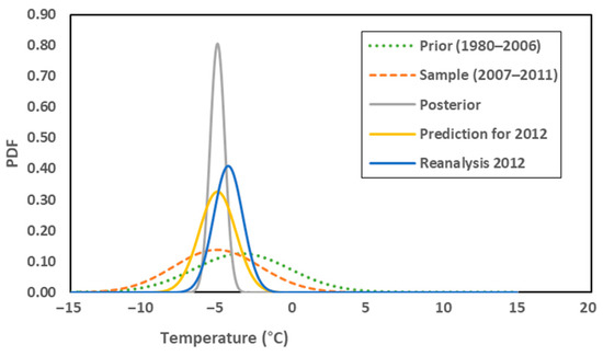
Figure 2.
Bayesian inference elements for daily average temperature of 1 April 2012, in coordinates (74.07° N, 35.81° E).
The monthly averages of the predicted meteorological and oceanographic conditions from different algorithms are compared with the reanalysis values in 2012, as shown in Figure 3, Figure 4, Figure 5, Figure 6, Figure 7 and Figure 8. Accordingly, there is no significant difference between the techniques and all of them demonstrate proper performance dealing with simulating meteorological and oceanographic conditions in the study area in the Arctic. However, the estimates of the Bayesian approach are slightly closer to the monthly average of the reanalysis values. Furthermore, examining the different number of iterations (i.e., and ) revealed the capabilities of both SIS and MCMC algorithms to simulate the meteorological and oceanographic conditions with a relatively low number of iterations while further iterations result in only small improvements in some cases.
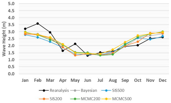
Figure 3.
Monthly average comparison between simulated and reanalysis values for wave height in coordinates (74.07° N, 35.81° E) in 2012.
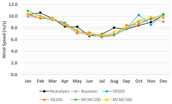
Figure 4.
Monthly average comparison between simulated and reanalysis values for wind speed in coordinates (74.07° N, 35.81° E) in 2012.
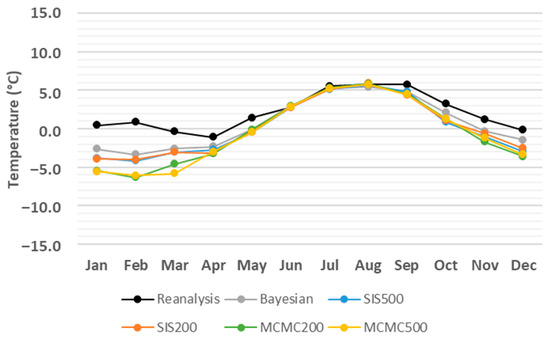
Figure 5.
Monthly average comparison between simulated and reanalysis values for temperature in coordinates (74.07° N, 35.81° E) in 2012.
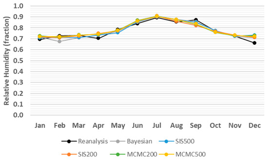
Figure 6.
Monthly average comparison between simulated and reanalysis values for relative humidity in coordinates (74.07° N, 35.81° E) in 2012.
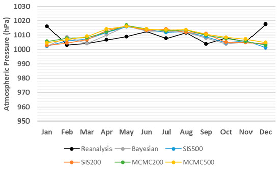
Figure 7.
Monthly average comparison between simulated and reanalysis values for atmospheric pressure in coordinates (74.07° N, 35.81° E) in 2012.
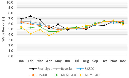
Figure 8.
Monthly average comparison between simulated and reanalysis values for wave period in coordinates (74.07° N, 35.81° E) in 2012.
Although Figure 3, Figure 4, Figure 5, Figure 6, Figure 7 and Figure 8 provide overviews of the performance of the algorithms dealing with the prediction of meteorological and oceanographic conditions in each month, the monthly average of the daily predicted values is not a proper measure to evaluate the deviation of the algorithms from the reanalysis values, since the positive and negative deviations offset each other. Therefore, to eliminate the offsetting effect, the absolute value of deviation for each day and each algorithm is taken and then the average absolute deviation (AAD) [38] for each month is calculated, which is the sum of the absolute values of the deviations from the reanalysis values, divided by the number of days in the month. Accordingly, the monthly AAD for different meteorological and oceanographic conditions are illustrated in Table 3, Table 4, Table 5, Table 6, Table 7 and Table 8. For further clarification, considering wave height as an example, Figure 3 indicates that comparing the monthly average of both the daily predicted values and the reanalysis values, the greatest deviation is 0.98 m related to SIS500 in February, whilst, Table 3 shows that, by eliminating the offsetting effect, the greatest monthly AAD is 1.48 m related to SIS200 in December. Thus, the least monthly AAD from the reanalysis values for wave height, wind speed, temperature, relative humidity, atmospheric pressure, and wave period are achieved by SIS200, MCMC500, MCMC500, MCMC500, SIS500, and Bayesian approach with the values of 0.38 m, 1.53 m/s, 0.57 °C, 4.88%, 4.2 hPa, and 0.6 s, respectively.
Table 3.
Monthly AAD 1 from reanalysis values for wave height (m) in coordinates (74.07° N, 35.81° E) in 2012, where the smallest value for each month is indicated in bold.
Table 4.
Monthly AAD from reanalysis values for wind speed (m/s) in coordinates (74.07° N, 35.81° E) in 2012, where the smallest value for each month is indicated in bold.
Table 5.
Monthly AAD from reanalysis values for temperature (°C) in coordinates (74.07° N, 35.81° E) in 2012, where the smallest value for each month is indicated in bold.
Table 6.
Monthly AAD from reanalysis values for relative humidity (fraction) in coordinates (74.07° N, 35.81° E) in 2012, where the smallest value for each month is indicated in bold.
Table 7.
Monthly AAD from reanalysis values for atmospheric pressure (hPa) in coordinates (74.07° N, 35.81° E) in 2012, where the smallest value for each month is indicated in bold.
Table 8.
Monthly AAD from reanalysis values for wave period (s) in coordinates (74.07° N, 35.81° E) in 2012, where the smallest value for each month is indicated in bold.
Considering the combination of 5 simulation techniques and 12 months, we have 72 scenarios for monthly AAD in 2012 of which in 35 scenarios the Bayesian approach has resulted in the lowest deviation from reanalysis value. This amount is 7, 10, 9, and 11 for SIS200, SIS500, MCMC200, and MCMC500, respectively. Therefore, the Bayesian approach is the most resistant technique, which is also robust due to few required assumptions for implementation.
Apart from the predicted meteorological and oceanographic conditions, some other parameters are required in the MINCOG model that are adopted from [39]. Accordingly, the salinity of seawater is kept constant at 35 ppt, the ship speed is 4 m/s, and surface seawater temperature is 2.5 °C. Additionally, winds and waves are coming from the same direction and the direction between wave and the ship is 150 degrees [39]. Eventually, the predicted meteorological and oceanographic conditions from different algorithms are separately plugged in the MINCOG model along with the adopted parameters as inputs to estimate the daily icing rate in coordinates (74.07° N, 35.81° E) in 2012. Consequently, the monthly average of icing rate is depicted in Figure 9 in which all of the techniques have led to competitive estimates quite close to the reanalysis values. Moreover, the monthly AAD from reanalysis values is indicated in Table 9, where the closest estimates to reanalysis values are related to Bayesian inputs followed by SIS200, SIS500, MCMC200, and MCMC500. Accordingly, the monthly AAD from reanalysis values for the MINCOG estimations with Bayesian inputs is not greater than 0.13 cm/h. Whilst, the largest monthly AAD from reanalysis values, yet competitive, is 0.41 cm/h related to MCMC200 inputs in February.
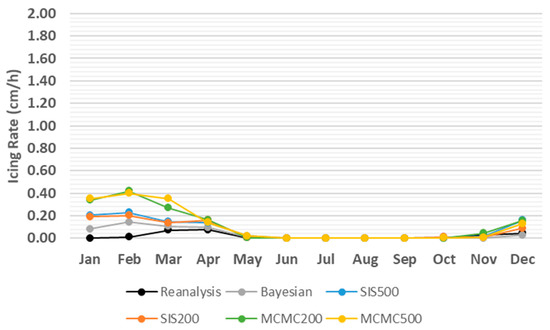
Figure 9.
Monthly average of icing rate (cm/h) using the Marine-Icing model for the Norwegian Coast Guard (MINCOG) model and simulated meteorological and oceanographic conditions as input parameters from different algorithms comparing with reanalysis values in coordinates (74.07° N, 35.81° E) in 2012.
Table 9.
Monthly AAD from reanalysis values for icing rate (cm/h) using MINCOG 1 model and simulated meteorological and oceanographic conditions as input parameters from different algorithms in coordinates (74.07° N, 35.81° E) in 2012, where the smallest value for each month is indicated in bold.
Additionally, the elapsed times of the Bayesian approach and simulation algorithms in the entire study area are illustrated in Table 10. Hence, the Bayesian framework is much faster than the other algorithms by the capability of predicting the six meteorological and oceanographic conditions for 366 days of the year 2012 in only 1 second for one location and 00:04:41 (i.e., 281 s) for the entire area. However, the running times of the other algorithms are quite low and competitive. The worst case in the simulation of the six meteorological and oceanographic conditions for one location in a year is related to SIS500 with 22 s. While in the simulation of the entire area, MCMC500 has the longest running time with 02:22:14. It should be mentioned that reading the data from the dataset and extracting the required information is a separate task, which lasts for about 1 minute for the entire area and is not affected by the algorithms. Likewise, simulating the daily icing rate for one year in the entire area by the MINCOG model takes around 16 hours that clearly is not influenced by the algorithms.
Table 10.
Elapsed time (hh:mm:ss) of the Bayesian approach and simulation algorithms in forecasting the six meteorological and oceanographic conditions.
4. Discussion
Warming in the Arctic is considerably higher than the global average level. As a result, traffic in the Arctic Ocean is growing rapidly [40], which is for purposes such as oil and gas discoveries, fishing, tourism, maritime trade, as well as research and investigation [1]. However, navigation in the Arctic Ocean is challenging due to harsh environmental conditions such as low temperatures, high-velocity winds, and ice on vessels. Ice on vessels is particularly known as a critical challenge since it may cause catastrophic consequences from safety and economic points of view [4,5].
Large, sophisticated computer models are routinely being used for forecasting the future of meteorological and oceanographic conditions based on the physics of the atmosphere and ocean. One drawback of these models is that they have been designed in a deterministic manner and uncertainty is not considered in their formulations. In other words, running the model with the same input parameters will always lead to the same result. In this regard, statistical tools provide promising approaches to deal quantitatively with chaotic events [19]. The other critical point in using such models is that lack of accuracy in the input parameters is a source of error in the results. Indeed, uncertainty in the inputs may be amplified by the model formulations and cause larger uncertainty in the outcome. In this view, it is expected that enhancing the accuracy of the input parameters improves the outcome of the model.
In former studies, the MINCOG model was developed for the simulation of sea spray icing on vessels [8,16]. However, for long-term prediction of sea spray ice, which is important from planning, safety, and financial viewpoints, meteorological and oceanographic conditions are required to be forecasted and plugged into the model as input parameters. To this aim, long-term prediction of meteorological and oceanographic conditions was mainly focused in this study.
As a matter of the climate change phenomenon, direct use of old historical data may not lead to proper predictions for the future. Therefore, a Bayesian approach was considered which modifies prior belief regarding data while receiving recently sampled data. Consequently, the posterior, which is a compromise of the prior and likelihood, provides a more reliable basis to build the prediction upon. Eventually, the results showed that the prior distribution was reasonably modified in terms of both central tendency and deviation.
Furthermore, simulation techniques comprised of SIS, and MCMC were investigated. In the proposed MCMC algorithm, predictions for a particular day are based on the history of the meteorological and oceanographic conditions in that day during the past 32 years. However, in the SIS algorithm, the predictions are according to the historical deviations from the previous day. A similar strategy regarding the target and the proposal densities was hired in SIS and MCMC. Accordingly, in both of the algorithms, the kernel density estimation was applied as a non-parametric solution for the target density and the Weibull distribution as the proposal density. Meanwhile, since the Weibull distribution does not support non-positive values, a data shifting procedure was embedded in the algorithms. The SIS algorithm iterates until a certain amount of samples are drawn. However, a second stopping criterion was considered in the MCMC algorithm to evaluate the convergence of the algorithm. Consequently, the standard SIS and MCMC were modified and the proposed algorithms were developed.
In order to verify the models, the data from 32 years (1980–2011) were used to predict the six meteorological and oceanographic conditions for one year on a daily basis and the results were compared with the 33rd year (2012). It is worth mentioning that the influence of the number of years that is used for prediction on daily AAD from reanalysis values was investigated. To this aim, two scenarios including 30 years and 32 years were compared via the two-sample t-test analysis for equality of the means. Accordingly, the results did not indicate a significant difference between the numbers of years that are chosen for prediction. The two-sample t-test analysis related to the prediction of wind speed by the MCMC500 algorithm is shown in Table 11. Thus, since the p-value is larger than the standard significance level of 0.05, the null hypothesis that the scenarios have similar results cannot be rejected.
Table 11.
Two-sample t-test analysis for equality of the means related to daily AAD from reanalysis values using MCMC500 algorithm considering 30 years and 32 years of data for prediction of wind speed (m/s) in coordinates (74.07° N, 35.81° E) in 2012.
Despite the capability of the algorithms in the long-term prediction of meteorological and oceanographic conditions, one drawback is that the conditions were separately predicted and the correlations between them were not examined. Considering the influences of the meteorological and oceanographic conditions on each other in the model design might lead to even better results. Thus, further investigation in this regard is suggested for later studies.
The variations of the monthly average of the icing rate are analogous to the variations of the input parameters. Generally, the deviation of predictions by the Bayesian framework is less than the other methods that cause less variation in the simulated icing rate. However, input parameters do not have the same contribution in the ice formation. However, it is suggested that wave height, wind speed, and temperature have higher contributions to the icing rate [16], and further statistical analysis in this regard is required. Moreover, to investigate the source of error and improve the algorithms, different aspects of the algorithms should be evaluated. For instance, the SIS and MCMC algorithms were designed using Weibull distribution with two sample sizes of 200 and 500. It is suggested to use other distribution functions such as normal to fit the data. Then, combinations of different distributions and stopping criteria should be evaluated. In this regard, statistical analysis methods such as the design of experiments (DOE), and the Taguchi method are recommended. Accordingly, the contributions of input parameters as well as the performance of each algorithm using combinations of different distributions and stopping criteria can be evaluated. Consequently, instead of using the predictions by a single algorithm as inputs for the MINCOG model, an optimal combination of algorithms can be applied.
5. Conclusions
This study proposes statistical methods for long-term prediction of meteorological and oceanographic conditions including wave height, wind speed, temperature, relative humidity, atmospheric pressure, and wave period, which are used as inputs in the MINCOG model to simulate sea spray icing for the future.
Meanwhile, 32 years (1980–2011) of reanalysis data from NORA10 was used to evaluate the performance of the models. Accordingly, four combinations of the proposed algorithms and sample sizes (i.e., SIS200, SIS500, MCMC200, and MCMC500), as well as the Bayesian framework, six meteorological and oceanographic conditions, were simulated for the year 2012 on a daily basis. Consequently, all the algorithms reached competitive results while the Bayesian model indicated slightly lower deviations from the reanalysis values in 2012. The Bayesian model was also much faster with the capability of predicting the six meteorological and oceanographic conditions for the entire area in less than five minutes. Therefore, the Bayesian approach is considered to be the most resistant technique, which is also robust due to few required assumptions for implementation. Moreover, the results implied that the proposed SIS and MCMC could properly cope with simulating the meteorological and oceanographic conditions in quite a low number of iterations (i.e., 200) while further iterations result in only little improvements. Hence, although SIS200 and MCMC200 take a longer time rather than the Bayesian framework, their running times for the entire area (i.e., <1 h and <1.5 h, respectively) are yet reasonable.
Eventually, the simulated values from all algorithms were considered as inputs in the MINCOG model to forecast the daily icing rate in 2012. Accordingly, the best results were obtained using Bayesian inputs closely followed by SIS200, SIS500, MCMC200, and MCMC500. The applied approaches and proposed models can play useful roles in industrial application, especially when new data and information are collected using which the meteorological and atmospheric conditions are predicted for future junctures. This provides the decision-maker with valuable information for planning offshore activities in the future (e.g., offshore fleet optimization). Accordingly, sea voyages with relatively lower risks can be selected based on the predicted meteorological and oceanographic conditions and icing rates. Further works can focus on developing a Bayesian approach using an empirical prior distribution rather than a Gaussian data-generating process. Moreover, the models can be combined with ant colony optimization (ACO), which is a promising approach to routing problems, in a multi-criteria decision-making (MCDM) framework to determine the shortest and safest sea routes for vessels. Moreover, the models can be embedded in planning and scheduling problems, such as maintenance scheduling in a dynamic condition to predict the possible intervals for maintenance activities.
Author Contributions
Conceptualization, A.S.B. and M.N.; methodology, A.S.B. and M.N.; software, A.S.B. and M.N.; validation, M.N.; formal analysis, A.S.B. and M.N.; investigation, A.S.B. and M.N.; resources, A.S.B. and M.N.; data curation, A.S.B. and M.N.; writing—original draft preparation, A.S.B.; writing—review and editing, M.N.; visualization, A.S.B. and M.N.; supervision, M.N.; project administration, M.N.; funding acquisition, M.N. All authors have read and agreed to the published version of the manuscript.
Funding
This research was funded by the High North Research Centre for Climate and the Environment (The Fram Centre), under Arctic Ocean Flagship under the project VesselIce.
Institutional Review Board Statement
Not applicable.
Informed Consent Statement
Not applicable.
Data Availability Statement
Restrictions apply to the availability of these data. Data was obtained from Norwegian Deepwater Programme (NDP) and are available at https://epim.no/ndp/ (accessed on 5 April 2021) with the permission of NDP.
Acknowledgments
The authors would like to acknowledge the Norwegian Deepwater Programme for the use of NORA10 hindcast data. The High North Research Centre for Climate and the Environment (The Fram Centre) is also acknowledged for financing this research. Moreover, the authors would like to express their gratitude to Eirik Mikal Samuelsen at the Norwegian Meteorological Institute as well as Truls Bakkejord Räder at SINTEF Nord AS for their wise ideas and useful comments during discussions and for providing valuable resources.
Conflicts of Interest
The authors declare no conflict of interest.
Abbreviations
| List of Acronyms. | |
| Acronym | Meaning |
| AAD | Average Absolute Deviation |
| ACO | Ant Colony Optimization |
| CV | Coefficient of Variation |
| DOE | Design of Experiments |
| IS | Importance Sampling |
| MCDM | Multi-Criteria Decision-Making |
| MCMC | Markov Chain Monte Carlo |
| MCMC200 | Markov Chain Monte Carlo with 200 iterations |
| MCMC500 | Markov Chain Monte Carlo with 500 iterations |
| MCS | Monte Carlo Simulation |
| MINCOG | Marine-Icing model for the Norwegian COast Guard |
| MLE | Maximum Likelihood Estimation |
| NORA10 | NOrwegian ReAnalysis 10 km |
| NSR | Northern Sea Route |
| RAMS | Reliability, Availability, Maintainability, and Safety |
| Probability Density Function | |
| RAMS | Reliability, Availability, Maintainability, and Safety |
| SIR | Sampling Importance Resampling |
| SIS | Sequential Importance Sampling |
| SIS200 | Sequential Importance Sampling with 200 iterations |
| SIS500 | Sequential Importance Sampling with 500 iterations |
| SMC | Sequential Monte Carlo |
| List of Symbols. | |
| Symbol | Meaning |
| The parameters of the Weibull distribution | |
| A positive value, which is needed to shift the data in Weibull estimation; since the Weibull distribution does not support non-positive values. | |
| CV for the last drawn samples in the MCMC algorithm iterations | |
| A threshold for CV | |
| The number of days in a year, which adopts the values 365 and 366 for normal and leap years, respectively. | |
| The daily mean of the parameter at time in year . Here, ‘time’ is referring to ‘day’. | |
| Deviation of from its value at time ‘’ in year . Here, ‘time’ is referring to ‘day’. | |
| The expected value of | |
| The expected value of a quantity of interest, , with respect to | |
| A target density | |
| Prior distribution of the parameter | |
| Posterior distribution of the parameter given the data | |
| The likelihood function of the data in hand, given the parameter | |
| Target density of a discrete-time sequential random variable at time | |
| Proposal density or envelope for | |
| Proposal density or envelope for | |
| An arbitrary function | |
| Indices for hyper-parameters | |
| H0 | The null hypothesis in the Anderson-Darling test of hypothesis |
| H1 | The alternative hypothesis in the Anderson-Darling test of hypothesis |
| Subscript index for samples; | |
| The weighted average of all drawn samples until iteration for , using IS weights | |
| Subscript index as iteration counter of algorithms; | |
| Center of the bin in the kernel density estimation | |
| Number of iterations of an algorithm | |
| MCMC estimation for at time | |
| Sample size | |
| p | The parameter of Binomial distribution |
| Possible values (i.e. state space) for the parameter in the SIS algorithm at time in year . Here, ‘time’ is referring to ‘day’. The values are based on the historical deviations from the daily mean of the parameter in the previous day. | |
| Sample standard deviation of | |
| Set of for all years; | |
| SIS estimation for at time | |
| Superscript index for the time in a discrete-time sequential process. Without loss of generality, ‘time’ is referring to ‘day’ in this study. | |
| IS weight for in a Markov process | |
| IS weight for in a Markov process for a drawn sample in iteration | |
| IS weight for a drawn sample in iteration | |
| IS weight for | |
| IS weight for in iteration | |
| Set of from iterations of SIS algorithm; | |
| The available data on the dataset | |
| The ith sample of | |
| Unobserved data of the random variable in the future | |
| A sample for | |
| Sample mean | |
| A random variable | |
| A discrete-time sequential random variable at time | |
| A discrete-time stochastic process representing the entire history of the sequence of a random variable | |
| A sample for | |
| The ith sample for | |
| Superscript index for years; | |
| Number of years from the dataset that are used for estimation | |
| Subscript index for bins in the kernel density estimation | |
| Acceptance probability in the Metropolis-Hastings algorithm | |
| Generic parameter that is supposed to be estimated | |
| A drawn sample for parameter , which might be accepted or rejected | |
| An accepted sample for parameter in iteration | |
| The parameter of Poisson distribution | |
| Mean of the data-generating process | |
| Hyper-parameters of Gaussian prior distribution | |
| Hyper-parameters of Gaussian posterior distribution | |
| Parameters of Gaussian predictive distribution | |
| Parameters of reanalysis values in 2012 | |
| The known variance of the data-generating process | |
References
- Sevastyanov, D.V. Arctic Tourism in the Barents Sea region: Current Situation and Boundaries of the Possible. Arct. North 2020, 39, 26–36. [Google Scholar] [CrossRef]
- Ryerson, C.C. Ice protection of offshore platforms. Cold Reg. Sci. Technol. 2011, 65, 97–110. [Google Scholar] [CrossRef]
- Dehghani-Sanij, A.R.; Dehghani, S.R.; Naterer, G.F.; Muzychka, Y.S. Sea spray icing phenomena on marine vessels and offshore structures: Review and formulation. Ocean Eng. 2017, 132, 25–39. [Google Scholar] [CrossRef]
- Heinrich, H. Industrial Accident Prevention: A Scientific Approach, 3rd ed.; McGraw Hill: New York, NY, USA, 1950. [Google Scholar]
- Chatterton, M.; Cook, J.C. The Effects of Icing on Commercial Fishing Vessels; Worcester Polytechnic Institute: Worcester, UK, 2008. [Google Scholar]
- Barabadi, A.; Garmabaki, A.; Zaki, R. Designing for performability: An icing risk index for Arctic offshore. Cold Reg. Sci. Technol. 2016, 124, 77–86. [Google Scholar] [CrossRef]
- Rashid, T.; Khawaja, H.A.; Edvardsen, K. Review of marine icing and anti-/de-icing systems. J. Mar. Eng. Technol. 2016, 15, 79–87. [Google Scholar] [CrossRef]
- Samuelsen, E.M.; Edvardsen, K.; Graversen, R.G. Modelled and observed sea-spray icing in Arctic-Norwegian waters. Cold Reg. Sci. Technol. 2017, 134, 54–81. [Google Scholar] [CrossRef]
- Mertins, H.O. Icing on fishing vessels due to spray. Mar. Obs. 1968, 38, 128–130. [Google Scholar]
- Stallabrass, J.R. Trawler Icing: A Compilation of Work Done at N.R.C.; Mechanical Engineering Report MD-56; National Research Conseil: Ottawa, ON, Canada, 1980. [Google Scholar]
- Sultana, K.R.; Dehghani, S.R.; Pope, K.; Muzychka, Y.S. A review of numerical modelling techniques for marine icing applications. Cold Reg. Sci. Technol. 2018, 145, 40–51. [Google Scholar] [CrossRef]
- Kulyakhtin, A.; Tsarau, A. A time-dependent model of marine icing with application of computational fluid dynamics. Cold Reg. Sci. Technol. 2014, 104–105, 33–44. [Google Scholar] [CrossRef]
- Horjen, I. Numerical Modelling of Time-Dependent Marine Icing, Anti-Icing and De-Icing; Norges Tekniske Høgskole (NTH): Trondheim, Norway, 1960. [Google Scholar]
- Horjen, I. Numerical modeling of two-dimensional sea spray icing on vessel-mounted cylinders. Cold Reg. Sci. Technol. 2013, 93, 20–35. [Google Scholar] [CrossRef]
- Forest, T.; Lozowski, E.; Gagnon, R.E. Estimating Marine Icing on Offshore Structures Using RIGICE04. In Proceedings of the 11th International Workshop on Atmospheric Icing of Structures, Montreal, PQ, Canada, 12–16 June 2005; National Research Council Canada: Montreal, QC, Canada, 2005; pp. 12–16. [Google Scholar]
- Samuelsen, E.M. Ship-icing prediction methods applied in operational weather forecasting. Q. J. R. Meteorol. Soc. 2017, 144, 13–33. [Google Scholar] [CrossRef]
- Reistad, M.; Breivik, Ø.; Haakenstad, H.; Aarnes, O.J.; Furevik, B.; Bidlot, J.R. A high-resolution hindcast of wind and waves for the North Sea, the Norwegian Sea, and the Barents Sea. J. Geophys. Res. Oceans 2011, 116, C05019. [Google Scholar] [CrossRef]
- Little, R.J. Calibrated Bayes: A Bayes/Frequentist Roadmap. Am. Stat. 2006, 60, 213–223. [Google Scholar] [CrossRef]
- Wilks, D. Statistical Methods in the Atmospheric Sciences, 3rd ed.; Academic Press: Cambridge, MA, USA, 2011; Volume 3. [Google Scholar]
- Park, M.H.; Ju, M.; Kim, J.Y. Bayesian approach in estimating flood waste generation: A case study in South Korea. J. Environ. Manag. 2020, 265, 110552. [Google Scholar] [CrossRef]
- Robert, C.; Casella, G. A Short History of Markov Chain Monte Carlo: Subjective Recollections from Incomplete Data. Stat. Sci. 2012, 26, 102–115. [Google Scholar] [CrossRef]
- Zio, E. The Monte Carlo Simulation Method for System Reliability and Risk Analysis; Springer: London, UK, 2013. [Google Scholar] [CrossRef]
- Epstein, E.S. Statistical Inference and Prediction in Climatology: A Bayesian Approach; Meteorological Monographs, American Meteorological Society: Boston, MA, USA, 1985; Volume 20. [Google Scholar]
- Lee, P.M. Bayesian Statistics, an Introduction, 2nd ed.; Wiley: New York, NY, USA, 1997. [Google Scholar]
- Barjouei, A.S.; Naseri, M.; Ræder, T.B.; Samuelsen, E.M. Simulation of Atmospheric and Oceanographic Parameters for Spray Icing Prediction. In Proceedings of the 30th Conference Anniversary of the International Society of Offshore and Polar Engineers, Shanghai, China, 11–16 October 2020; ISOPE: Mountain View, CA, USA, 2020; ISOPE-I-20-1256; pp. 750–1256. Available online: https://onepetro.org/ISOPEIOPEC/proceedings-abstract/ISOPE20/All-ISOPE20/ISOPE-I20-1256/446378 (accessed on 20 April 2021).
- Ridgeway, G.; Madigan, D. A Sequential Monte Carlo Method for Bayesian Analysis of Massive Datasets. Data Min. Knowl. Discov. 2003, 7, 301–319. [Google Scholar] [CrossRef] [PubMed]
- Givens, G.H.; Hoeting, J.A. Computational Statistics, 2nd ed.; John Wiley & Sons Inc.: Hoboken, NJ, USA, 2013. [Google Scholar] [CrossRef]
- Rubin, D.B. Comment. J. Am. Stat. 1987, 82, 543–546. [Google Scholar] [CrossRef]
- Rubin, D.B. Using the SIR algorithm to simulate posterior distributions. In Bayesian Statistics 3; Bernardo, J.M., DeGroot, M.H., Lindley, D.V., Smith, A.F., Eds.; John Wiley & Sons Inc.: Oxford, UK, 1988; pp. 395–402. [Google Scholar]
- Liu, J.S.; Chen, R. Sequential Monte Carlo Methods for Dynamic Systems. J. Am. Stat. Assoc. 1988, 93, 1032–1044. [Google Scholar] [CrossRef]
- Barbu, A.; Zhu, S.C. Sequential Monte Carlo. In Monte Carlo Methods; Springer: Singapore, 2020; pp. 19–48. [Google Scholar] [CrossRef]
- Brooks, S.P.; Roberts, G.O. Convergence assessment techniques for Markov chain Monte Carlo. Stat. Comput. 1998, 8, 319–335. [Google Scholar] [CrossRef]
- Tierney, L. Markov Chains for Exploring Posterior Distributions. Ann. Stat. 1994, 22, 1701–1762. [Google Scholar] [CrossRef]
- Cowles, M.K.; Carlin, B.P. Markov Chain Monte Carlo Convergence Diagnostics: A Comparative Review. J. Am. Stat. Assoc. 1996, 91, 883–904. [Google Scholar] [CrossRef]
- Norwegian Petroleum Directorate. Available online: https://factpages.npd.no/en (accessed on 4 May 2020).
- Anderson, T.W.; Darling, D.A. Asymptotic theory of certain ‘goodness-of-fit’ criteria based on stochastic processes. Ann. Math. Stat. 1952, 23, 193–212. [Google Scholar] [CrossRef]
- MATLAB. MATLAB and Simulink; 9.8.0.1396136 (R2020a); The MathWorks Inc.: Natick, MA, USA, 2020; Available online: https://es.mathworks.com/products/matlab/ (accessed on 14 April 2020).
- Smith, G. Essential Statistics, Regression, and Econometrics, 2nd ed.; Academic Press: Cambridge, MA, USA, 2015. [Google Scholar] [CrossRef]
- Naseri, M.; Samuelsen, E.M. Unprecedented Vessel-Icing Climatology Based on Spray-Icing Modelling and Reanalysis Data: A Risk-Based Decision-Making Input for Arctic Offshore Industries. Atmosphere 2019, 10, 197. [Google Scholar] [CrossRef]
- Wang, S.; Mu, Y.; Zhang, X.; Jia, X. Polar tourism and environment change: Opportunity, impact and adaptation. Polar Sci. 2020, 25, 100544. [Google Scholar] [CrossRef]
Publisher’s Note: MDPI stays neutral with regard to jurisdictional claims in published maps and institutional affiliations. |
© 2021 by the authors. Licensee MDPI, Basel, Switzerland. This article is an open access article distributed under the terms and conditions of the Creative Commons Attribution (CC BY) license (https://creativecommons.org/licenses/by/4.0/).