Author Contributions
A.I.: Conceptualization, Methodology, Software, Investigation, Resources, Data curation, Writing—original draft preparation, Writing—review and editing, Visualization, Project administration, Funding acquisition; U.D.N.: Conceptualization, Methodology, Writing—review and editing, Supervision, Project administration; K.K.H.: Conceptualization, Resources, Writing—review and editing, Supervision, Project administration; J.D.: Conceptualization, Writing—review and editing, Supervision, Project administration; R.G.: Conceptualization, Writing—review and editing, Supervision, Project administration. All authors have read and agreed to the published version of the manuscript.
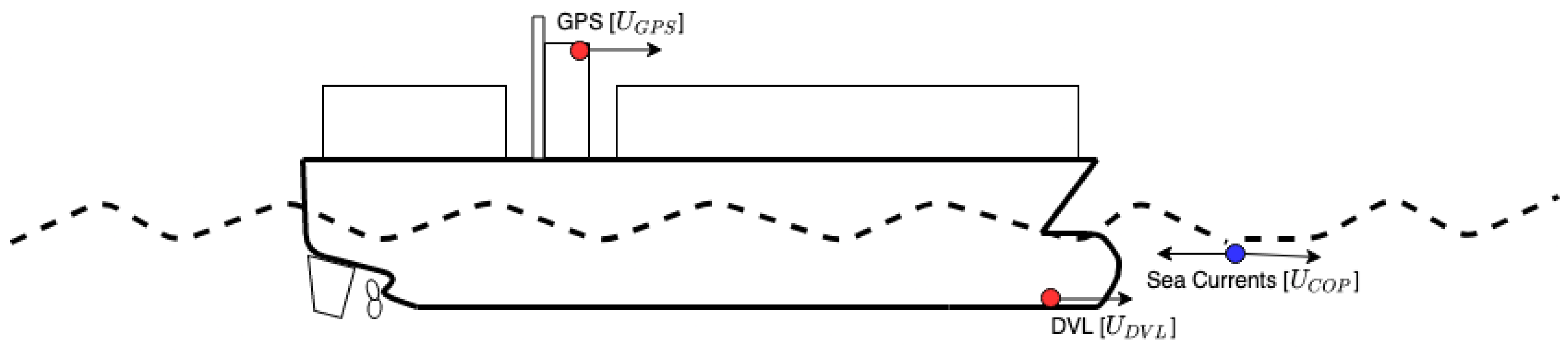
Figure 1.
Locations where the three speed signals of interest derive from. Red is used to indicate ship sensors and blue for predictions.
Figure 1.
Locations where the three speed signals of interest derive from. Red is used to indicate ship sensors and blue for predictions.
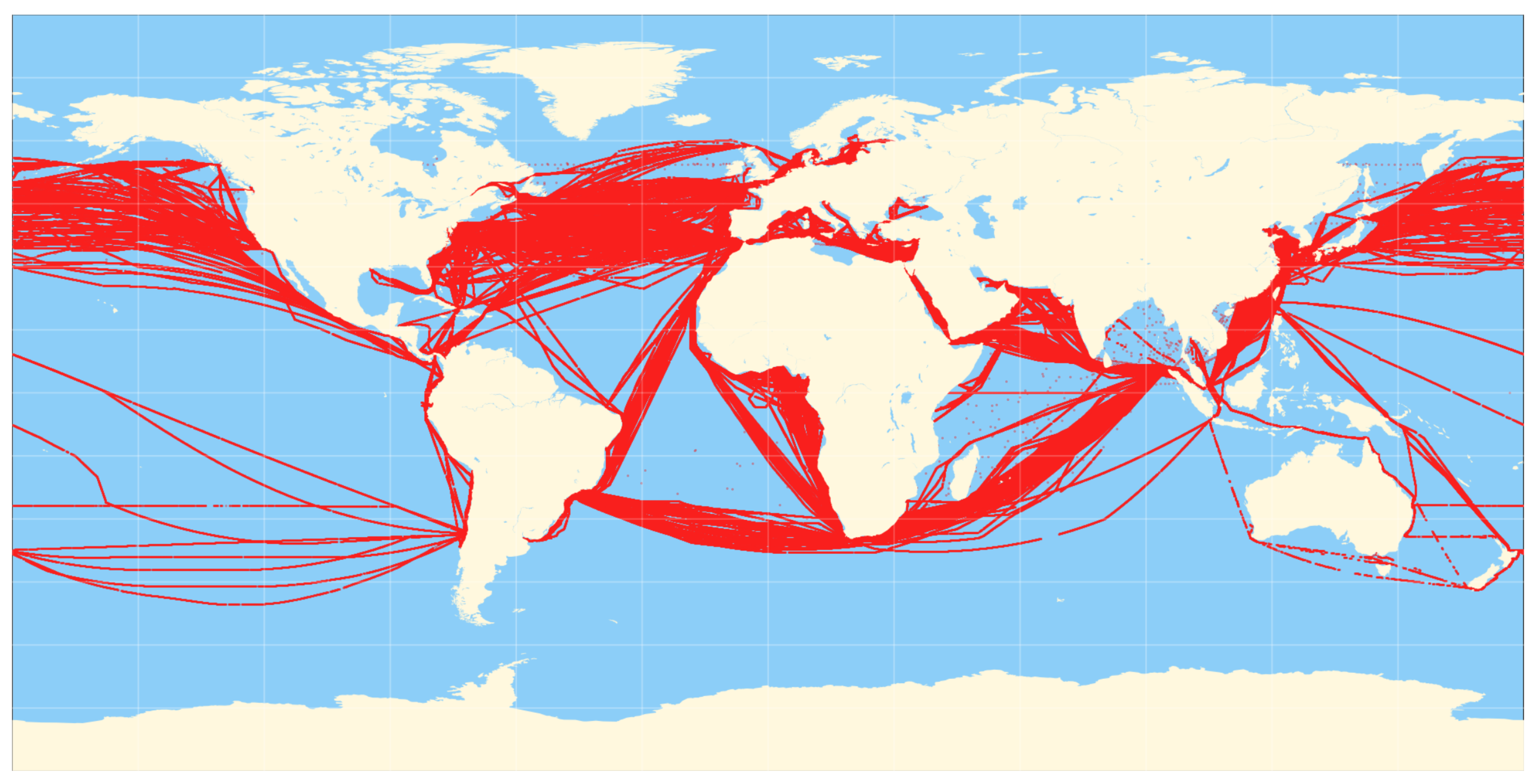
Figure 2.
Visualization of and coordinate pairs from all ships included in the main dataset for 3 years of operation.
Figure 2.
Visualization of and coordinate pairs from all ships included in the main dataset for 3 years of operation.
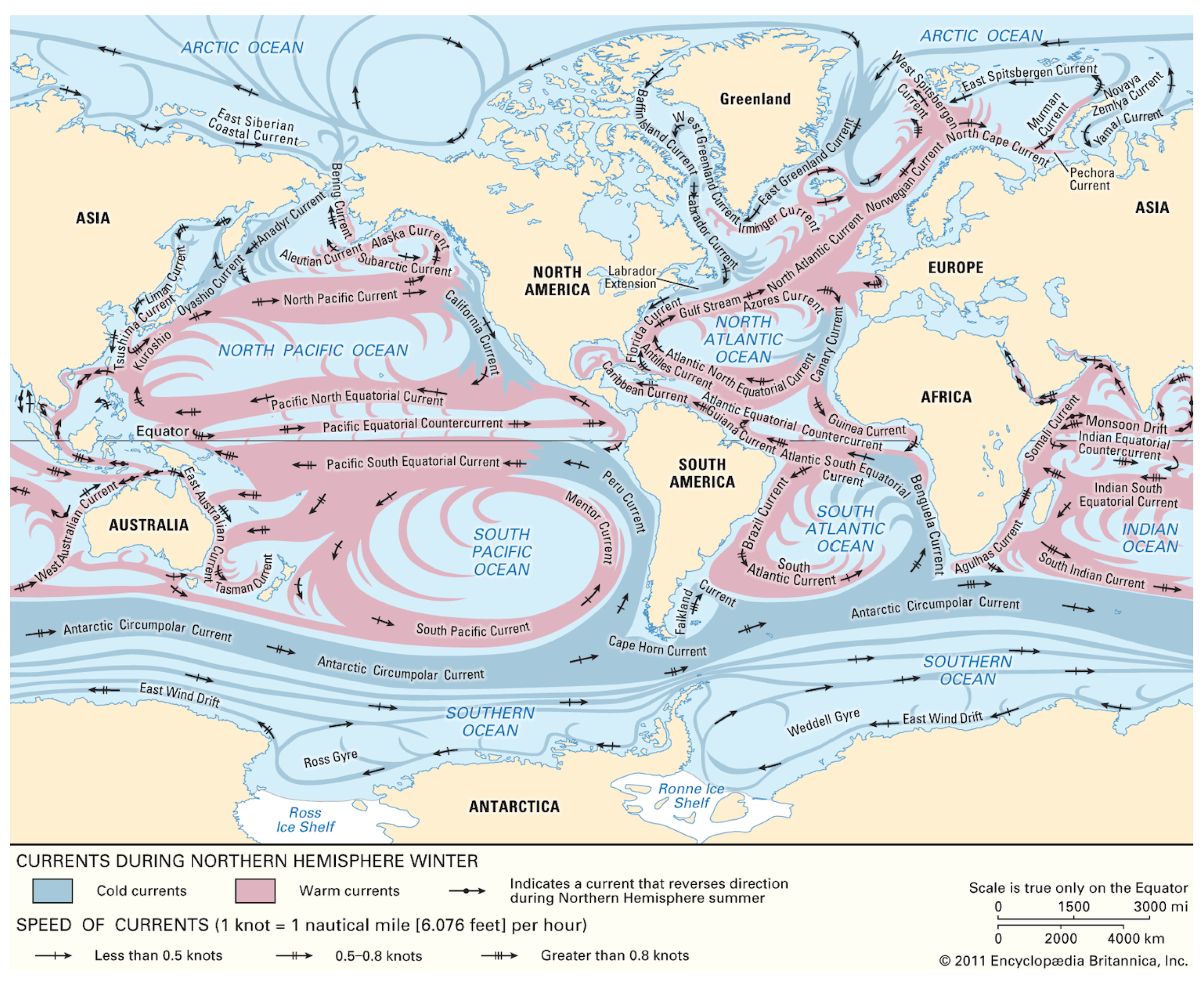
Figure 3.
Global surface currents magnitude during northern hemisphere winter by [
22].
Figure 3.
Global surface currents magnitude during northern hemisphere winter by [
22].
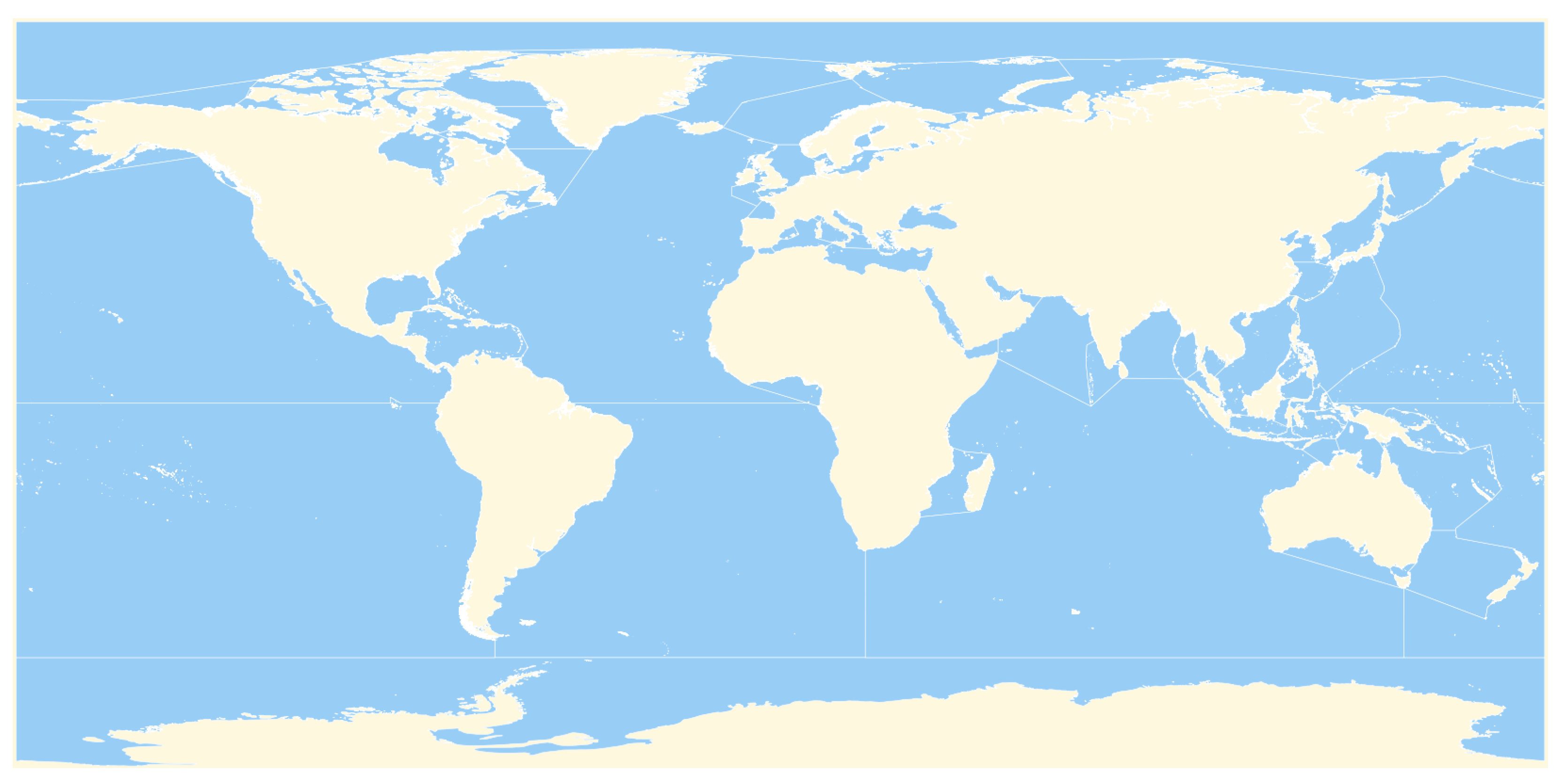
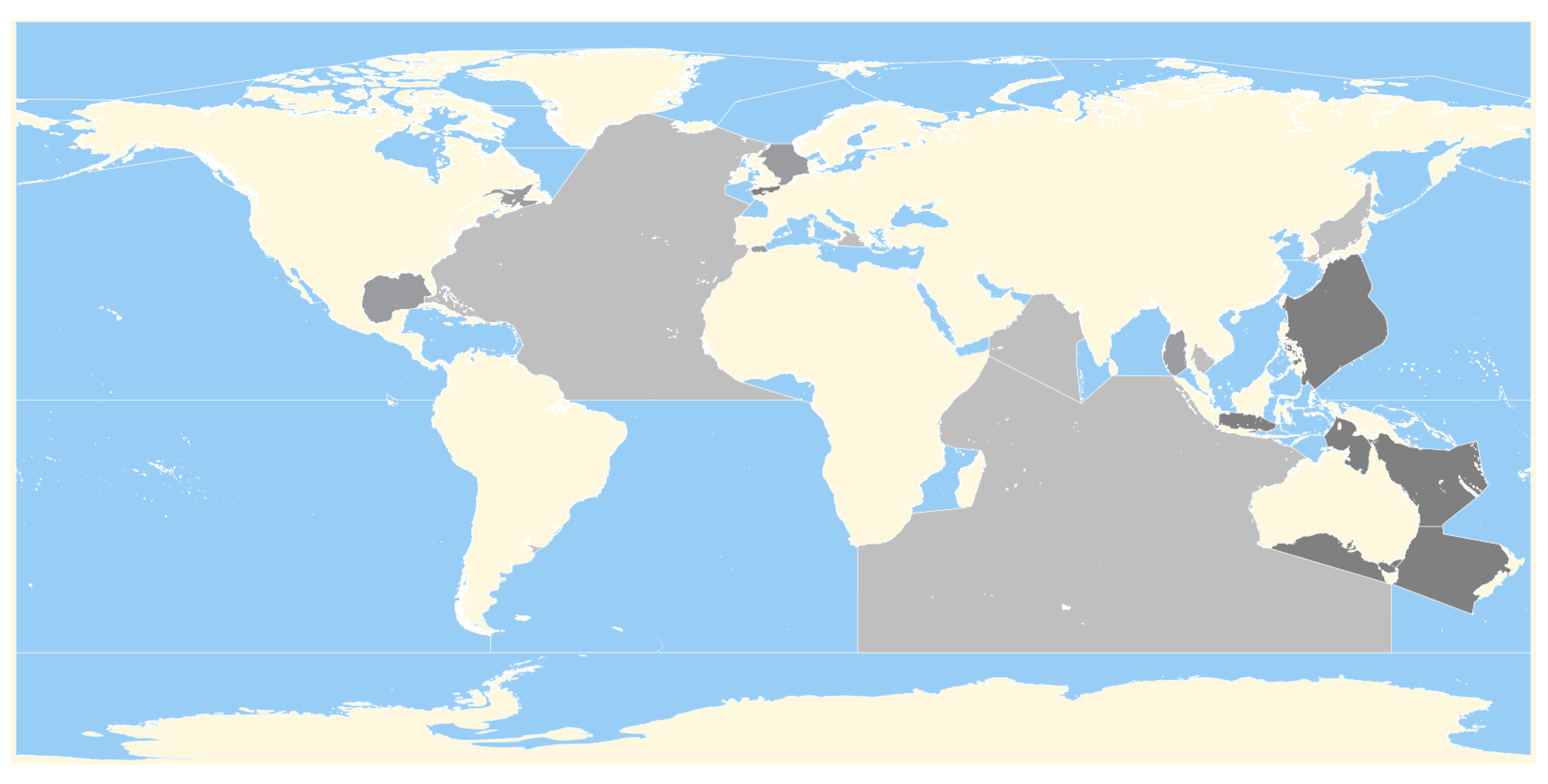
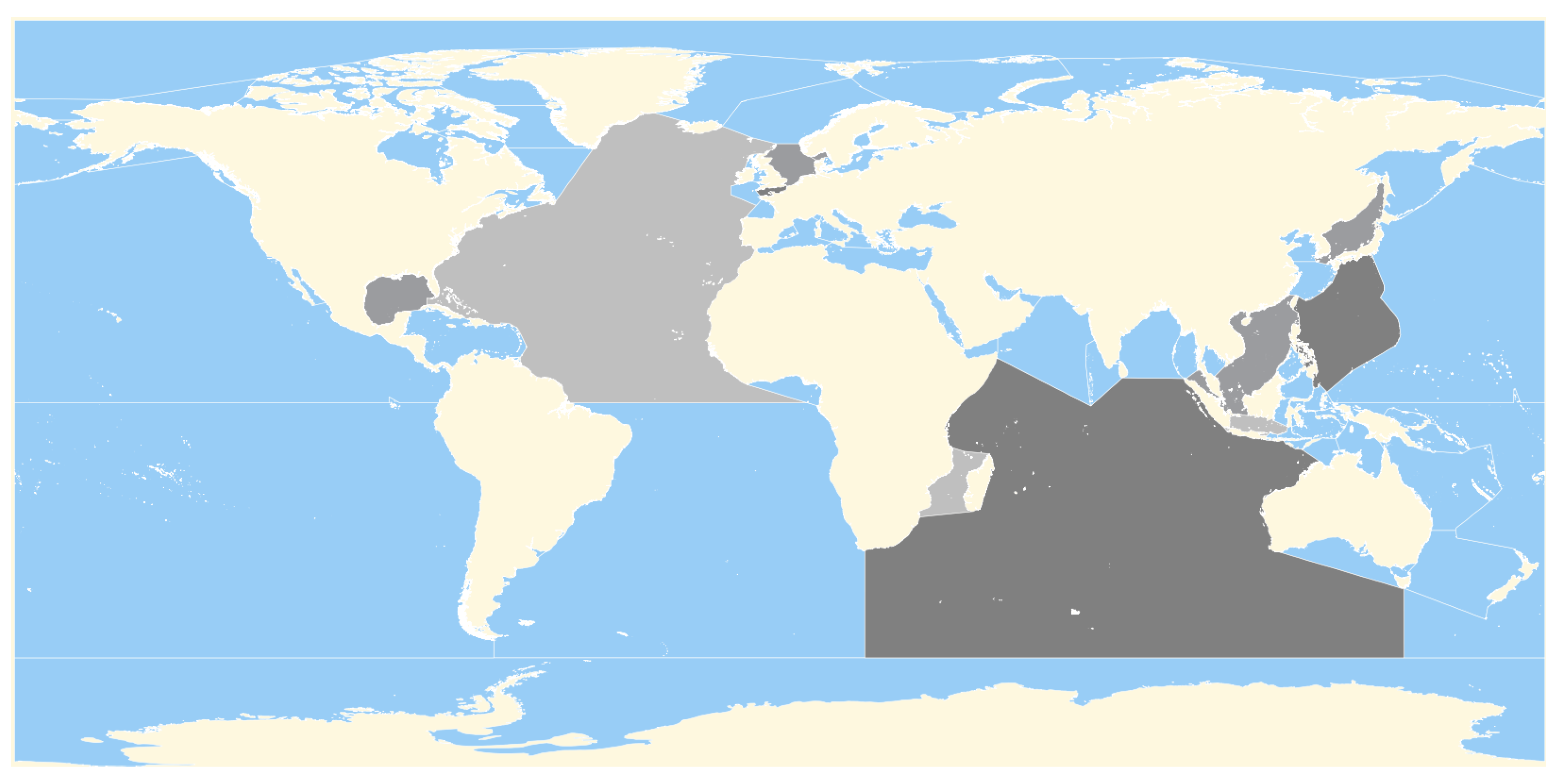
Figure 4.
The IHO seas regions of the world.
Figure 4.
The IHO seas regions of the world.
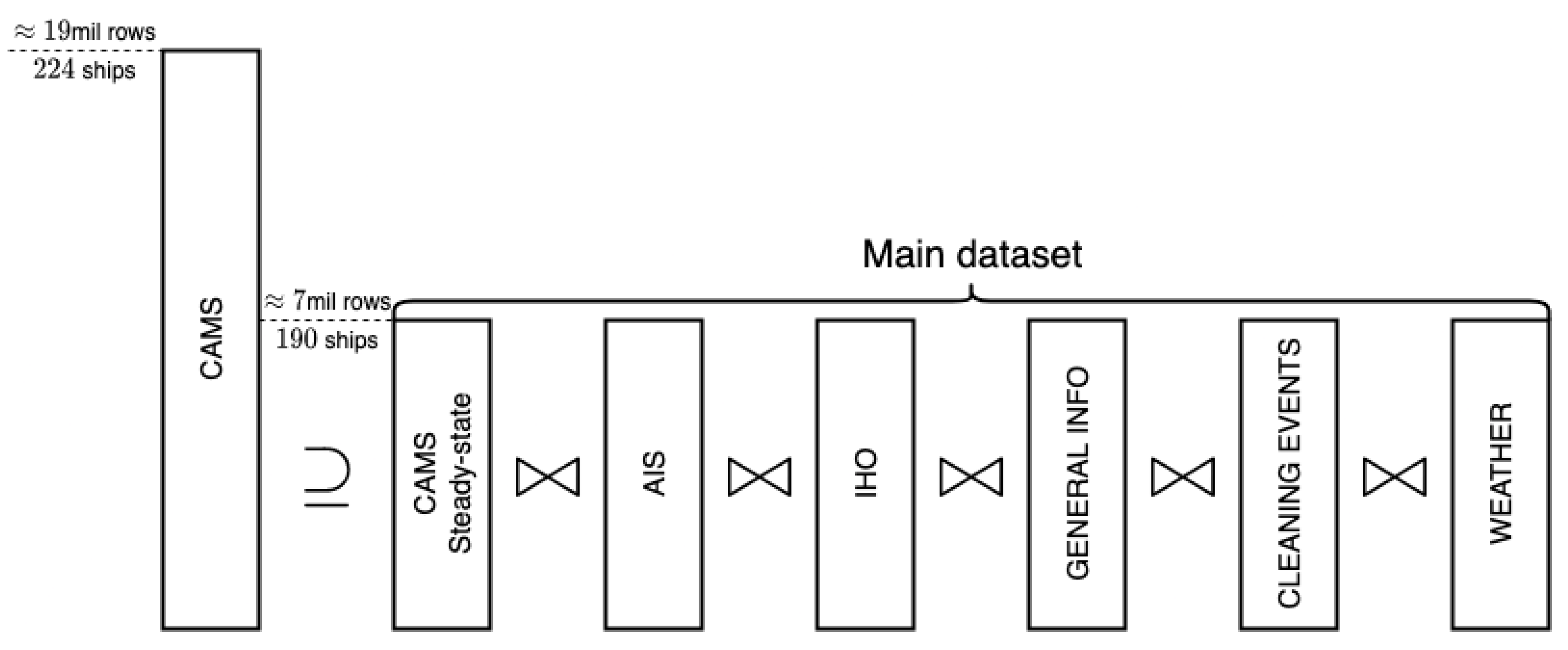
Figure 5.
An illustration of the merging procedure of the data sources.
Figure 5.
An illustration of the merging procedure of the data sources.
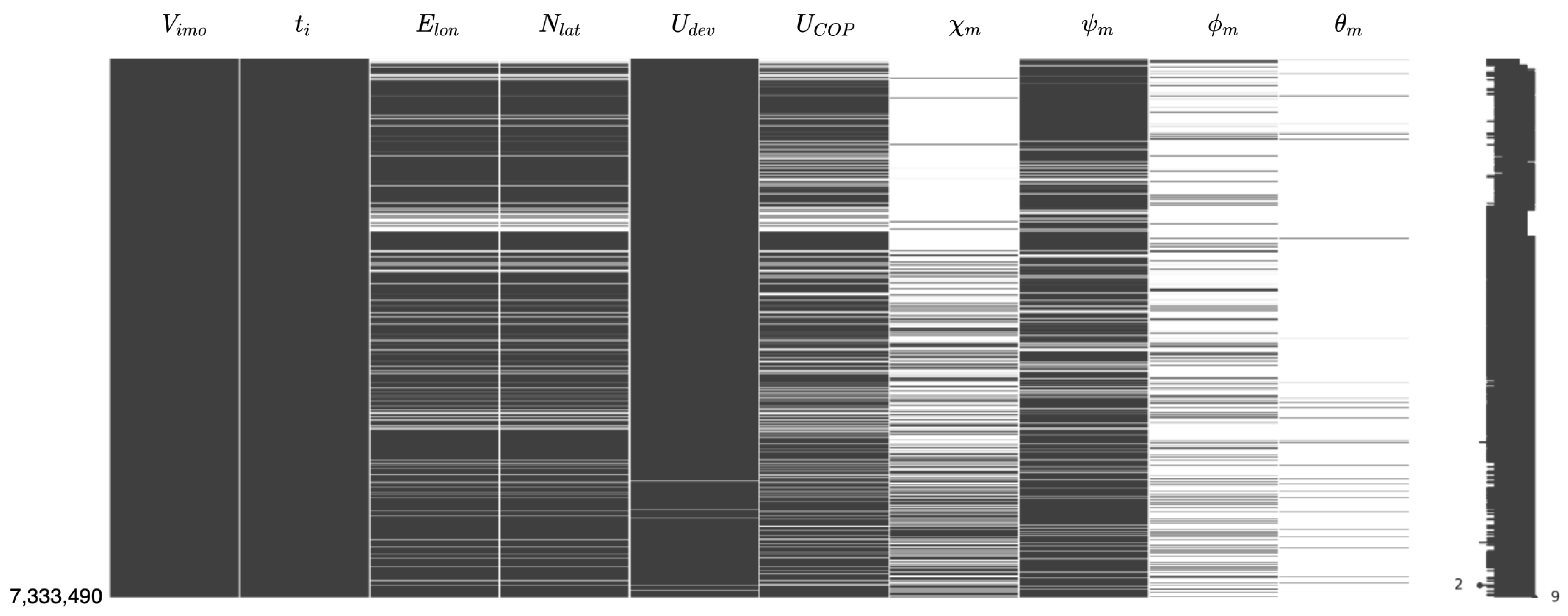
Figure 6.
Missing data matrix for the principal features of the main dataset.
Figure 6.
Missing data matrix for the principal features of the main dataset.
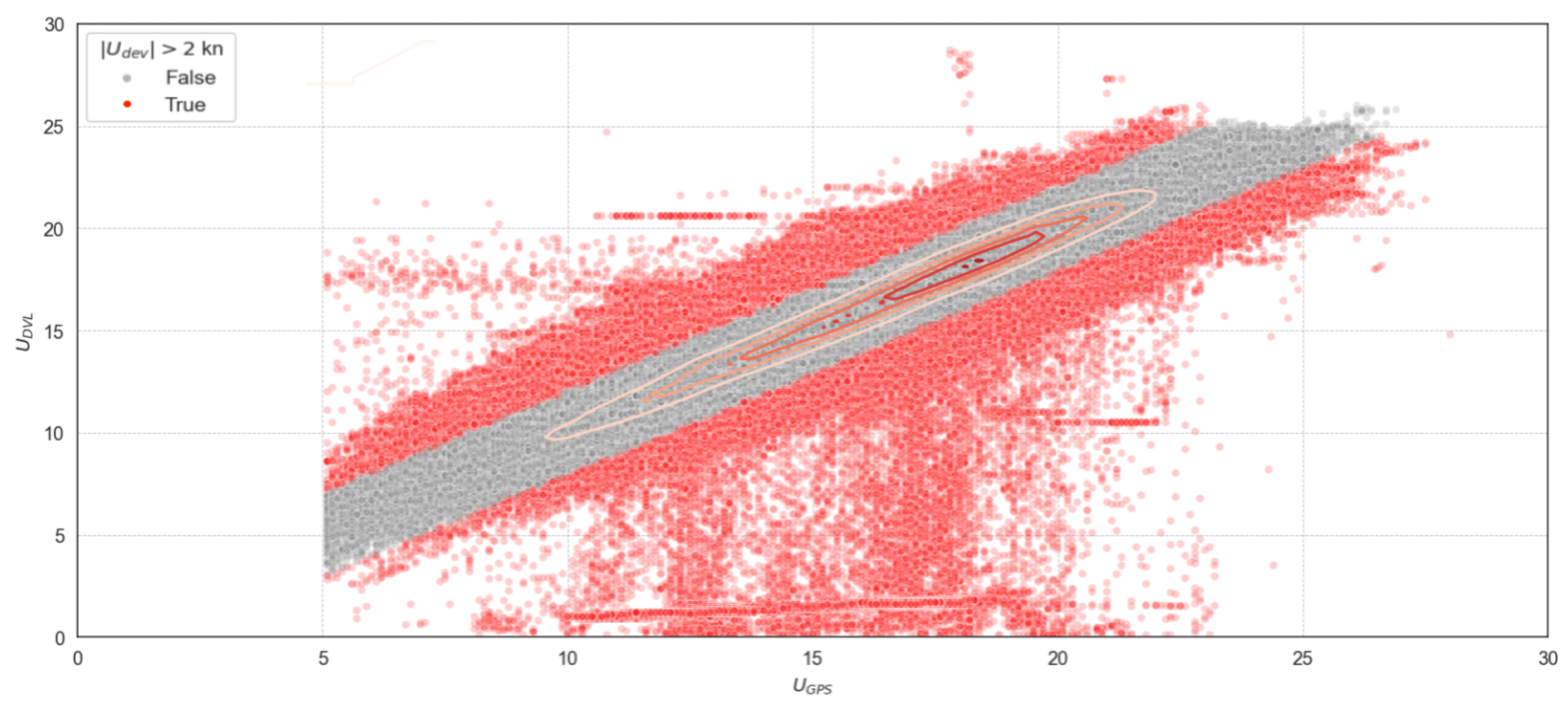
Figure 7.
KDE plot on top of correlation scatterplot of versus from 190 container ships.
Figure 7.
KDE plot on top of correlation scatterplot of versus from 190 container ships.
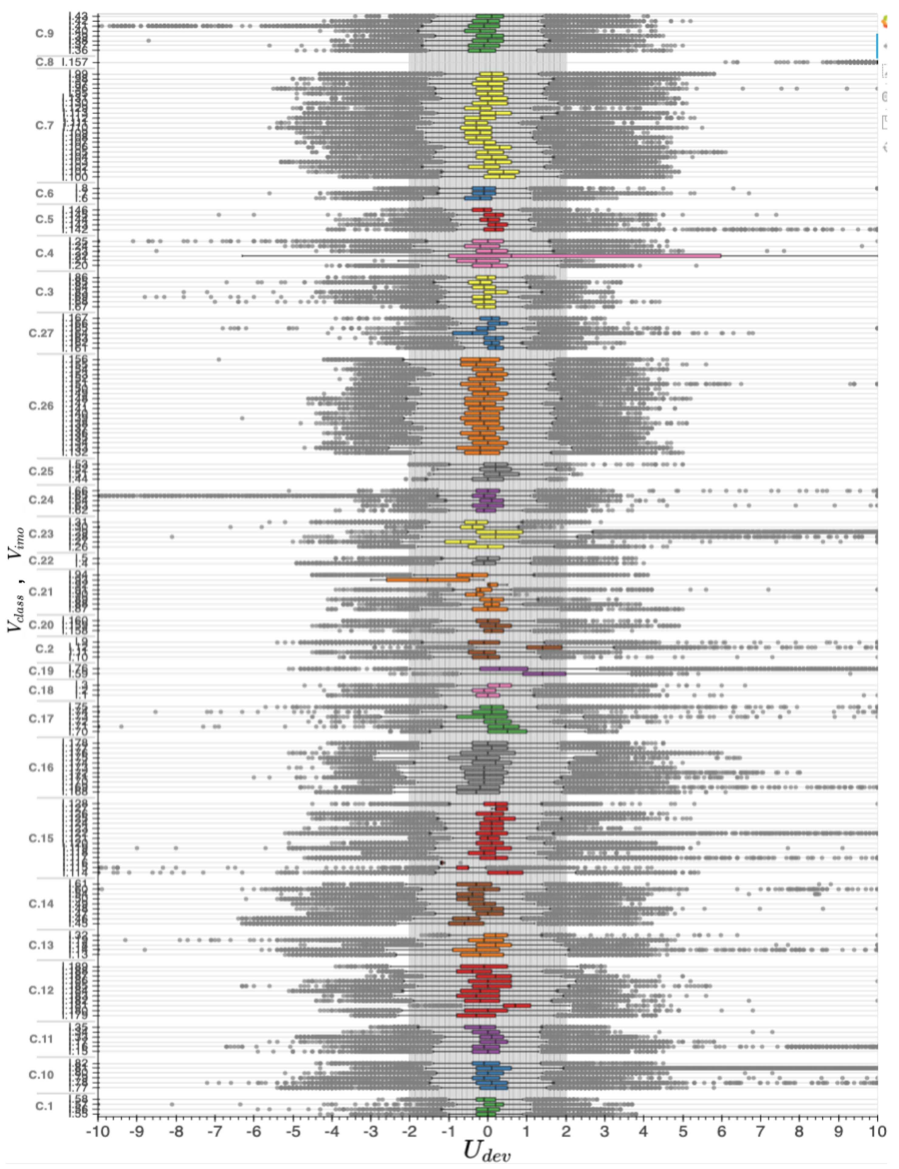
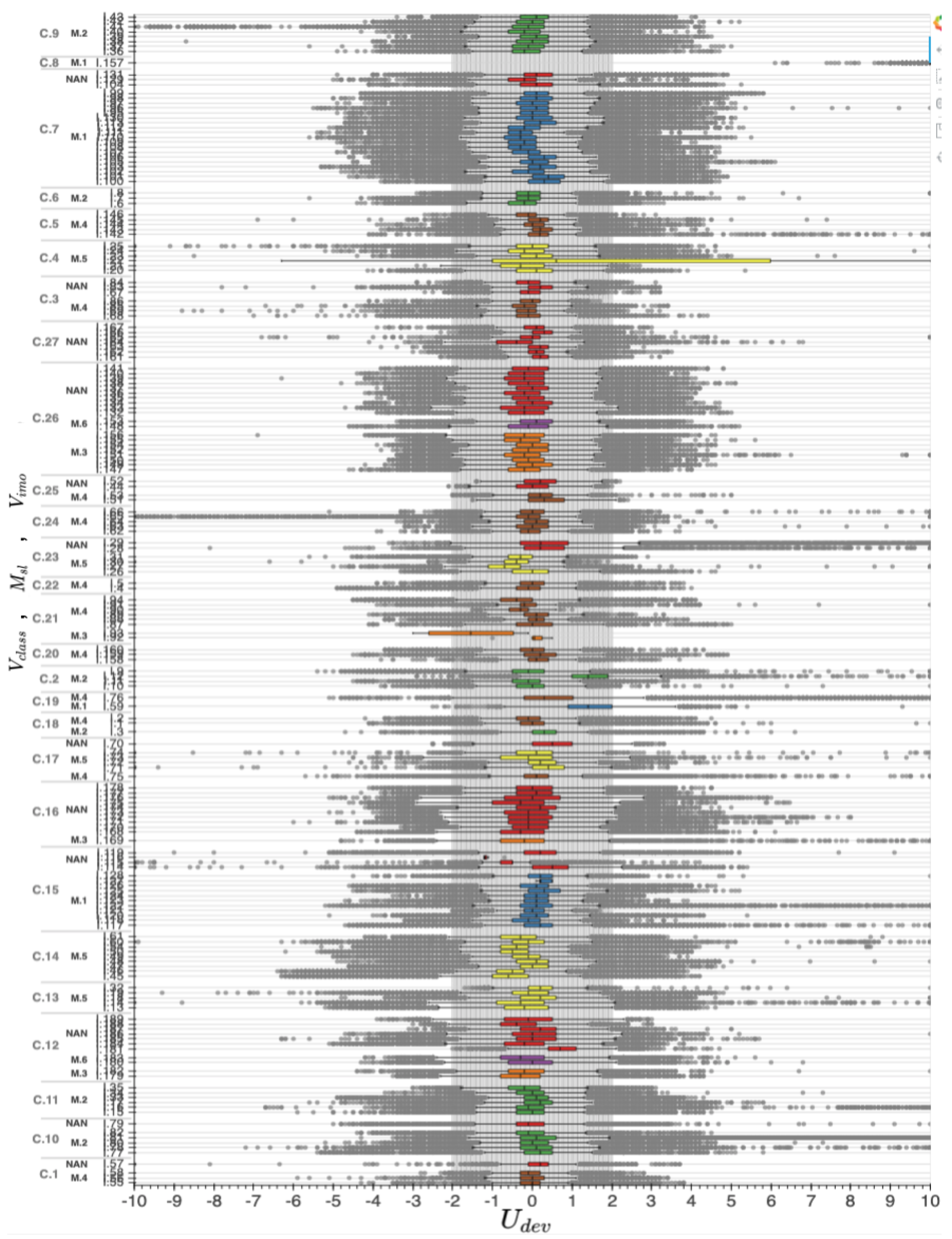
Figure 8.
Boxplot of by vessel class and IMO number .
Figure 8.
Boxplot of by vessel class and IMO number .
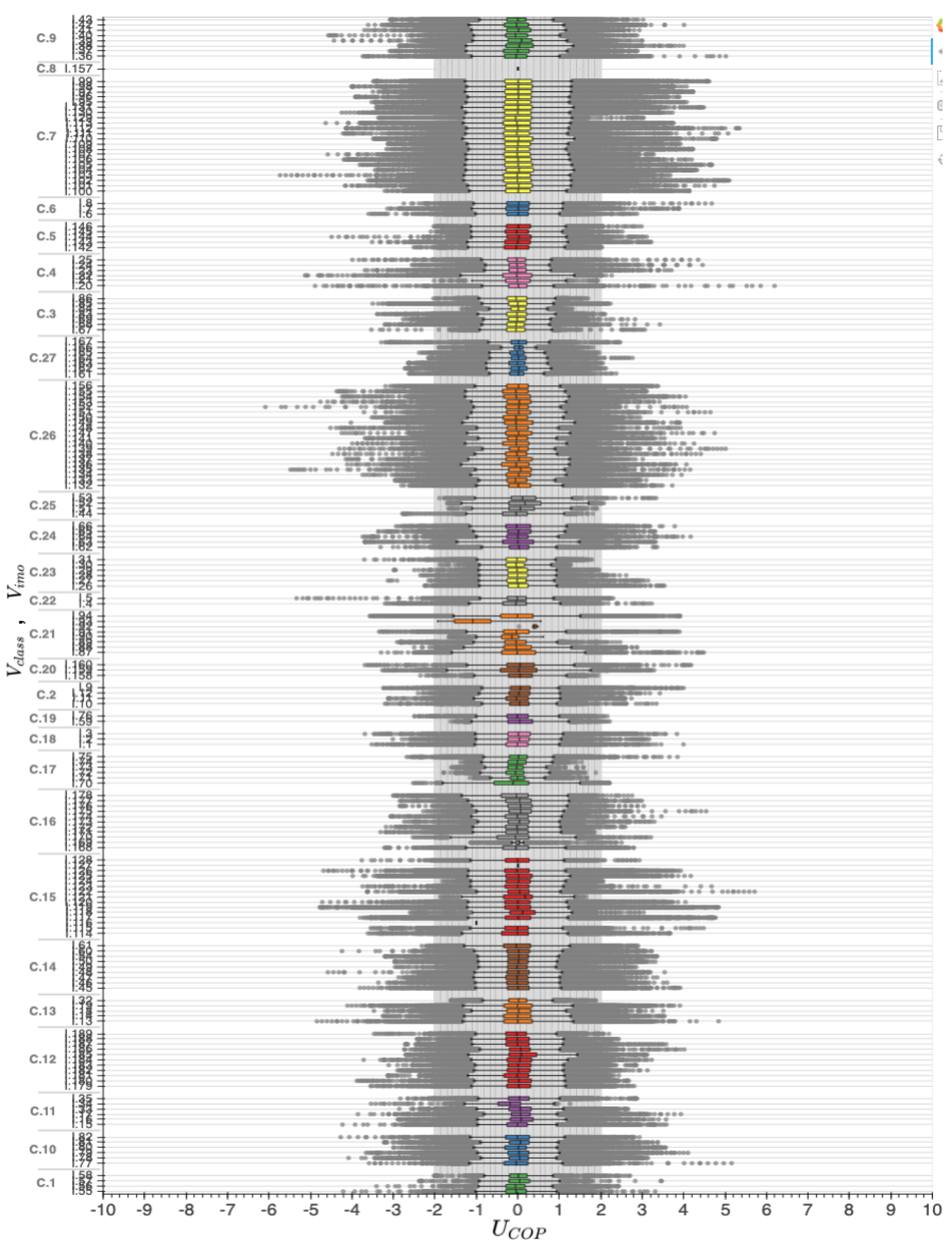
Figure 9.
Boxplot of by vessel class , DVL manufacturer and imoNo .
Figure 9.
Boxplot of by vessel class , DVL manufacturer and imoNo .
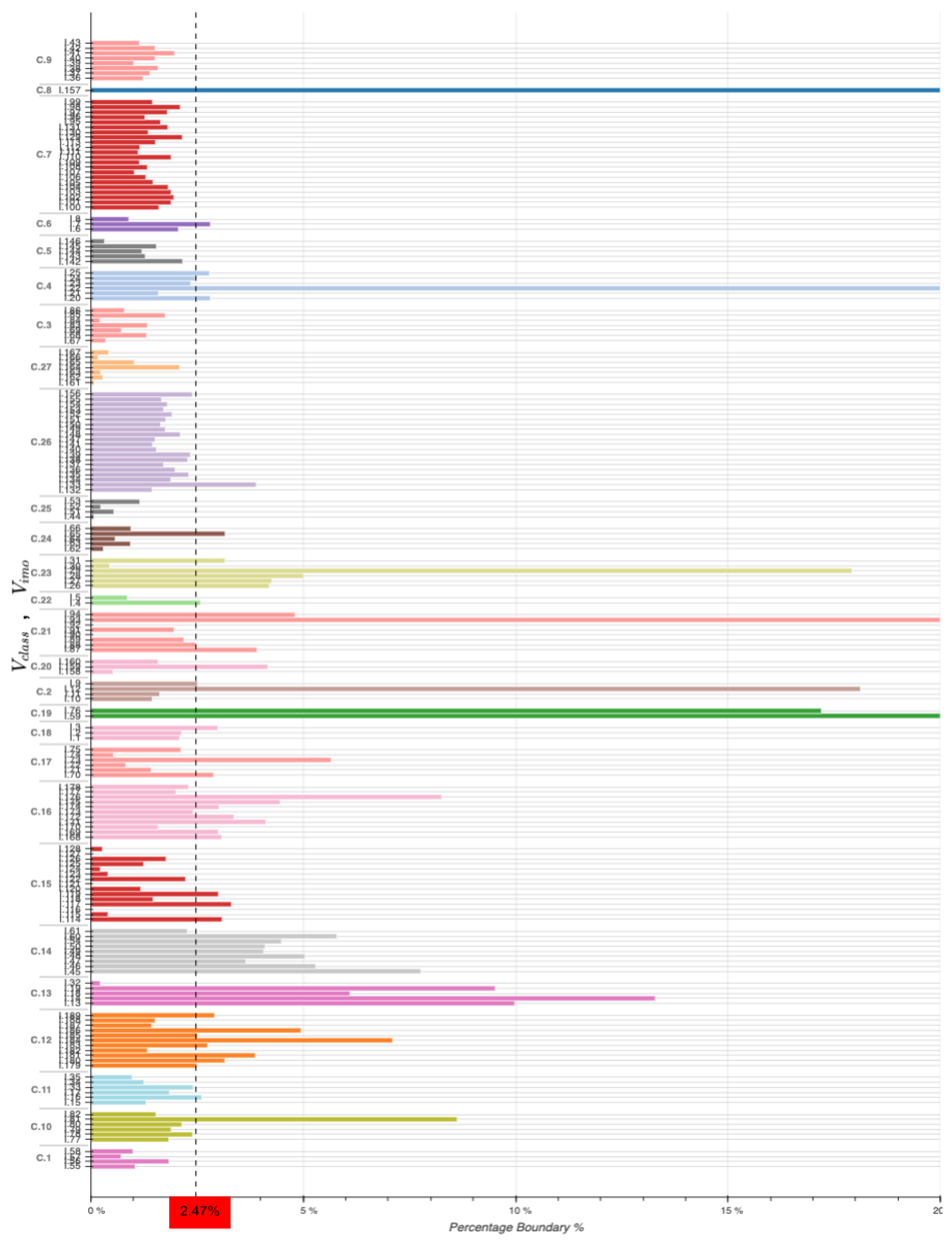
Figure 10.
Barplot of boundary percentage by vessel class and IMO number .
Figure 10.
Barplot of boundary percentage by vessel class and IMO number .
Figure 11.
The IHO seas regions of the world. The regions are gray when the percentage column of kn is greater than and it gets darker when it increases.
Figure 11.
The IHO seas regions of the world. The regions are gray when the percentage column of kn is greater than and it gets darker when it increases.
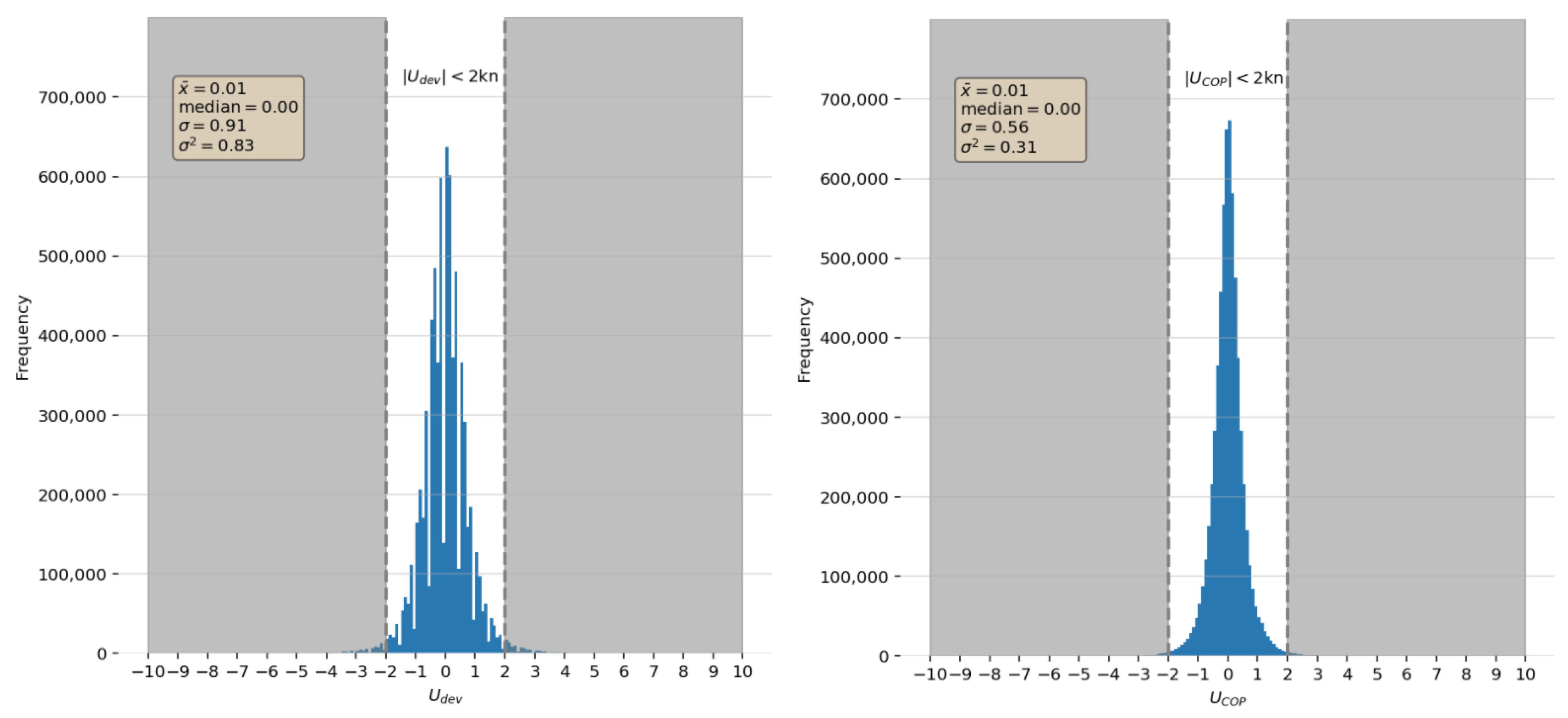
Figure 12.
Distribution histograms of and for 190 container ships.
Figure 12.
Distribution histograms of and for 190 container ships.
Figure 13.
Distribution boxplots of and for 190 container ships.
Figure 13.
Distribution boxplots of and for 190 container ships.
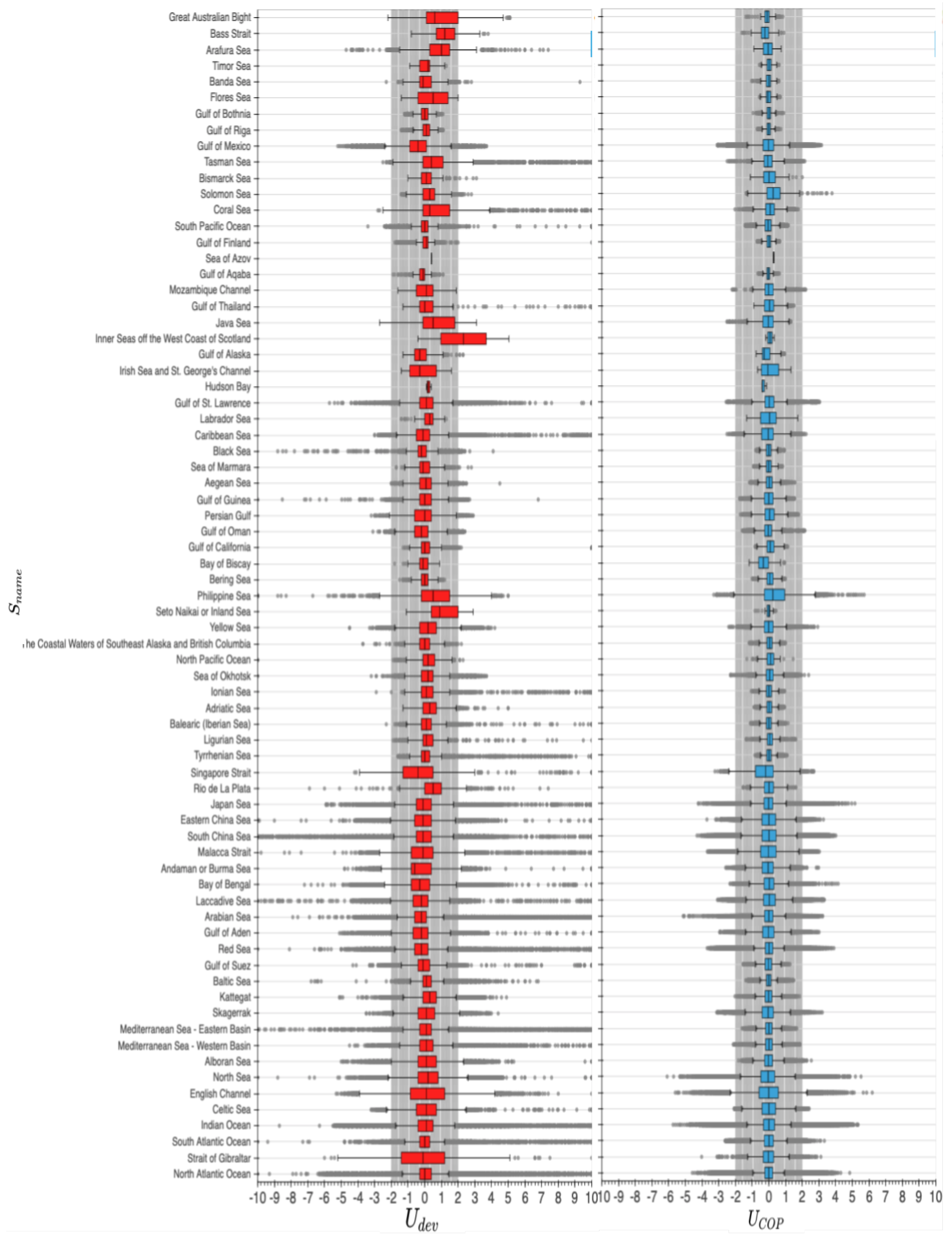
Figure 14.
Barplots of and by sea name .
Figure 14.
Barplots of and by sea name .
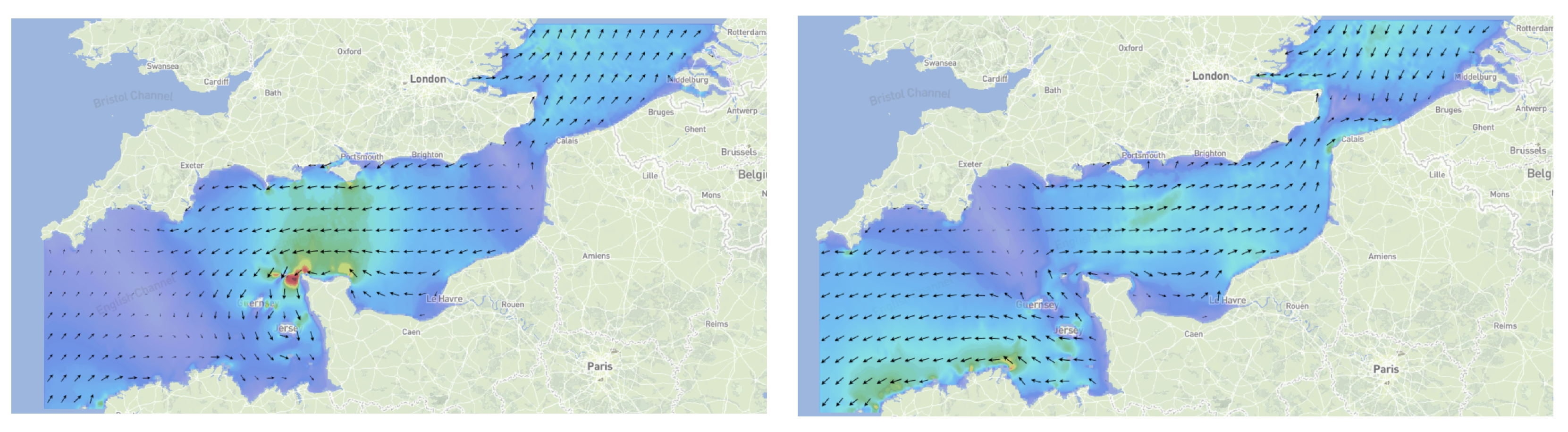
Figure 15.
Snapshots of the English Channel sea currents
with 2-h difference from one another, by [
35].
Figure 15.
Snapshots of the English Channel sea currents
with 2-h difference from one another, by [
35].
Figure 16.
The IHO seas regions of the world. The regions are gray when the percentage column of kn is greater than and it gets darker when it increases.
Figure 16.
The IHO seas regions of the world. The regions are gray when the percentage column of kn is greater than and it gets darker when it increases.
Figure 17.
Boxplot of by vessel class and IMO number .
Figure 17.
Boxplot of by vessel class and IMO number .
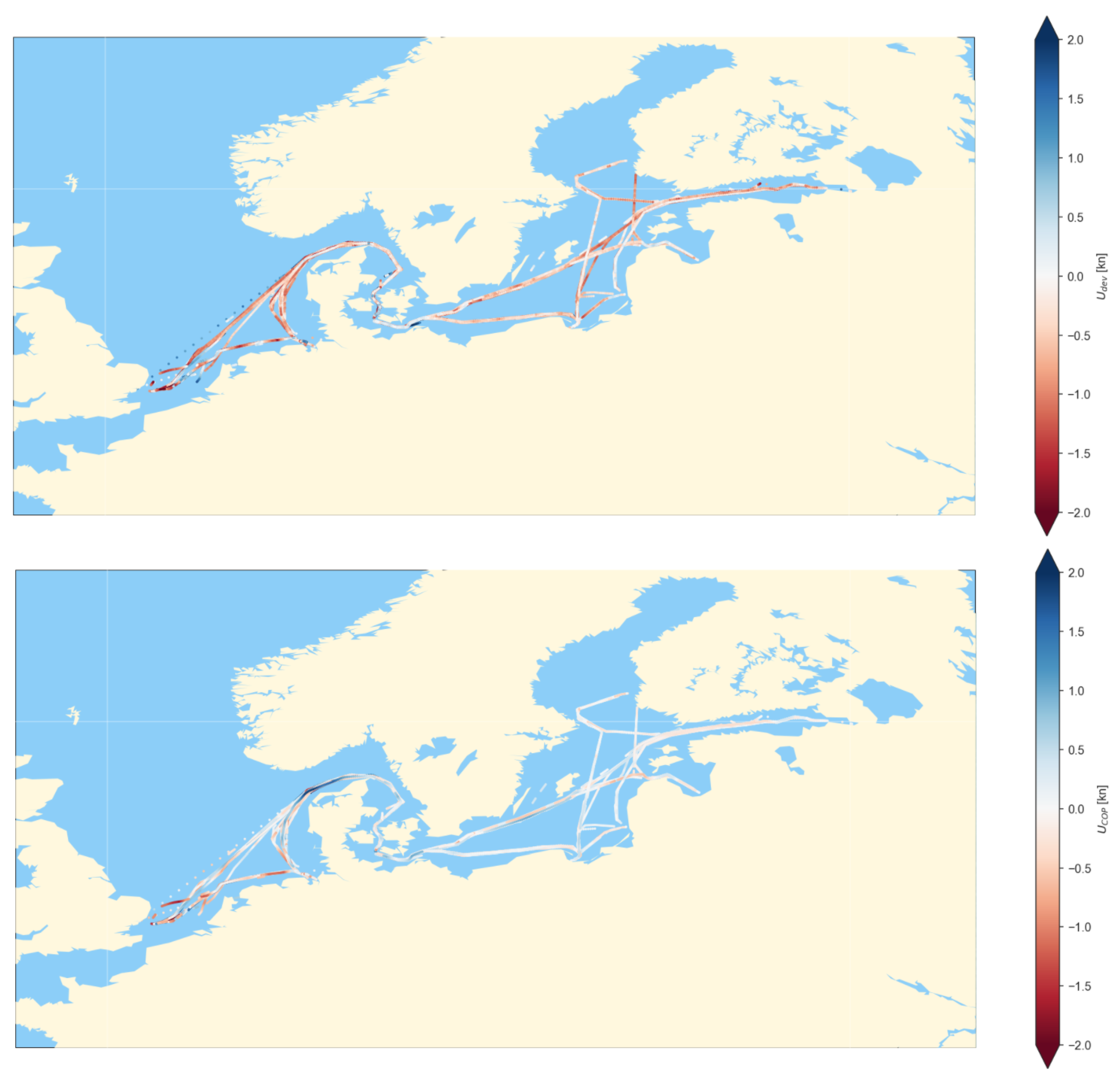
Figure 18.
Full journey of a C.27 class ship from 04/12/2018 to 22/02/2020. Upper map shows a density plot of where on the bottom map, the same for .
Figure 18.
Full journey of a C.27 class ship from 04/12/2018 to 22/02/2020. Upper map shows a density plot of where on the bottom map, the same for .
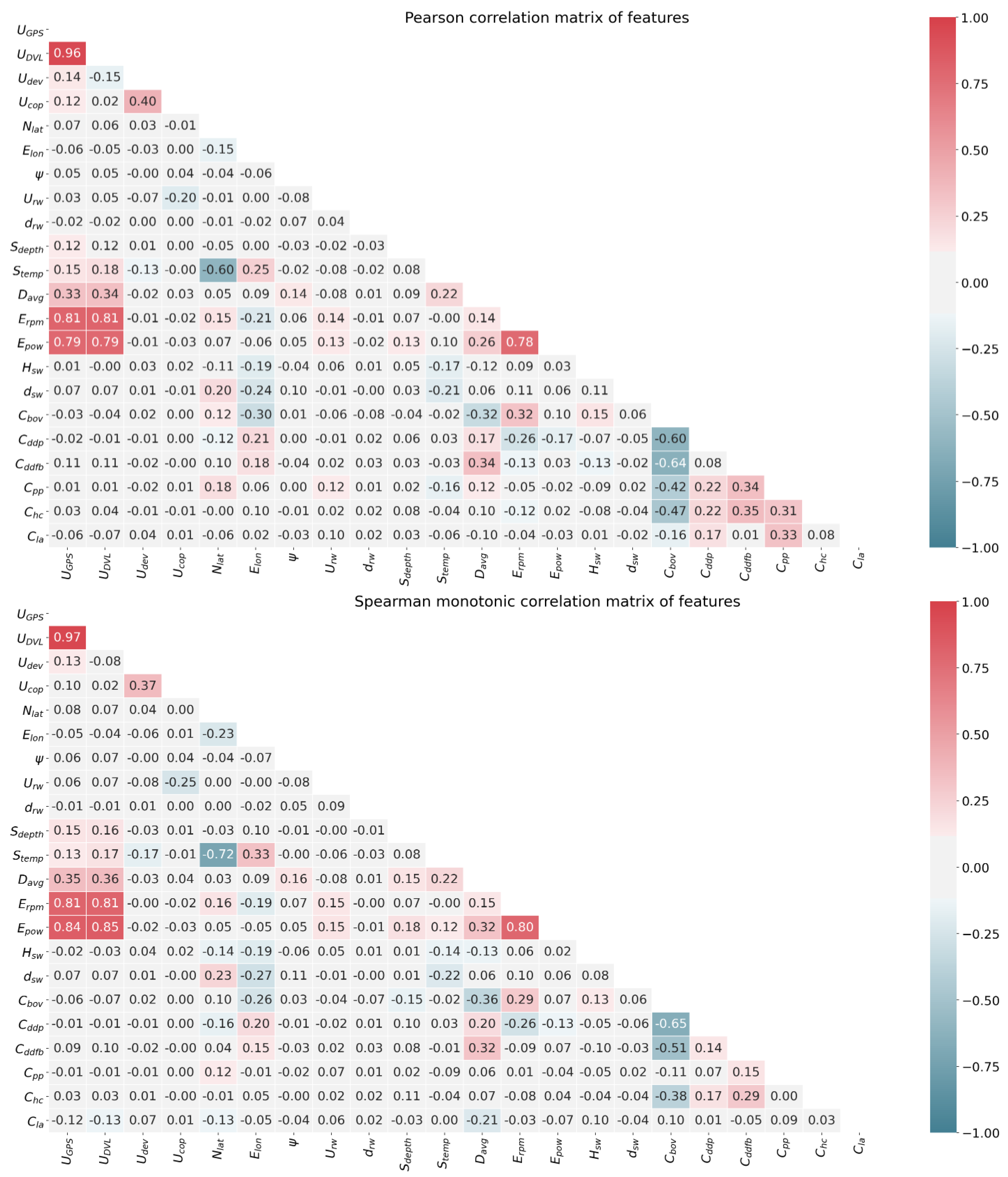
Figure 19.
Pearson and Spearman correlation matrices of the continuous features of the main dataset.
Figure 19.
Pearson and Spearman correlation matrices of the continuous features of the main dataset.
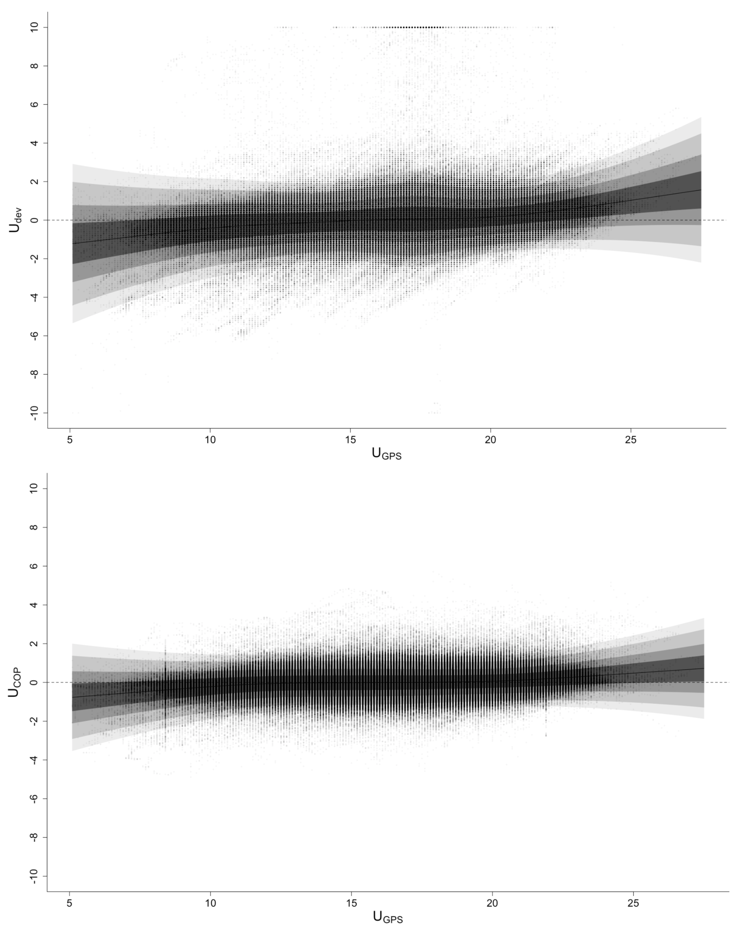
Figure 20.
Linear correlation density scatterplot of versus the rest of the continuous features of the main dataset.
Figure 20.
Linear correlation density scatterplot of versus the rest of the continuous features of the main dataset.
Figure 21.
GAMLSS multiplot of versus the rest of the continuous features of the main dataset.
Figure 21.
GAMLSS multiplot of versus the rest of the continuous features of the main dataset.
Figure 22.
Centile curves using GAMLSS of and over as explanatory variable for the main dataset.
Figure 22.
Centile curves using GAMLSS of and over as explanatory variable for the main dataset.
Table 1.
Estimated accuracy (
) of motion and weather signals, according to manufacturers or weather providers’ documentation [
19,
20,
21].
Table 1.
Estimated accuracy (
) of motion and weather signals, according to manufacturers or weather providers’ documentation [
19,
20,
21].
| Signal | Accuracy [] |
|---|
| |
| |
| |
| |
Table 2.
Sampling frequency, acquisition range and units of CAMS data.
Table 2.
Sampling frequency, acquisition range and units of CAMS data.
| Condition | Type | Frequency | Range | Unit |
|---|
| Loading | Draught Aft | Hz | 0–30 | [m] |
| Draught Fore | Hz | 0–30 | [m] |
| Operational | GPS Timestamp | Hz | 14/12/2016–22/02/2020 | [UTC datetime] |
| Latitude | Hz | –90 | [] |
| Longitude | Hz | –180 | [] |
| Shaft speed | Hz | –300 | [rpm] |
| ME Power | Hz | 0–100,000 | [kW] |
| Longitudinal STW | Hz | –50 | [kn] |
| GPS SOG | Hz | –50 | [kn] |
| True heading | Hz | 0–360 | [] |
| Course over ground | Hz | 0–360 | [] |
| Roll | Hz | –90 | [] |
| Pitch | Hz | –90 | [] |
| Water Depth (Under Keel) | Hz | 0–11,000 | [m] |
| Weather | True Wind Speed | Hz | 0–50 | [m/s] |
| True wind direction | Hz | 0–360 | [] |
| Relative wind speed | Hz | 0–50 | [m/s] |
| Relative wind direction | Hz | 0–360 | [] |
| Sea temperature | Hz | –100 | [°C] |
Table 3.
Sampling frequency, acquisition range and units of AIS data.
Table 3.
Sampling frequency, acquisition range and units of AIS data.
| Condition | Type | Frequency | Range | Unit |
|---|
| Loading | Draught Avg | uneven | 0–30 | [m] |
| Operational | AIS Timestamp | uneven | 01/10/2017–10/03/2020 | [UTC datetime] |
| AIS SOG | uneven | –50 | [kn] |
| Latitude | uneven | –90 | [] |
| Longitude | uneven | –180 | [] |
| True heading | uneven | 0–360 | [] |
| Course over ground | uneven | 0–360 | [] |
Table 4.
Sampling frequency, range and units of IHO seas data.
Table 4.
Sampling frequency, range and units of IHO seas data.
| Condition | Type | Frequency | Range | Unit |
|---|
| Sea info | Sea name | 1 name/sea | 148 seas worldwide. | [-] |
| Geometry | 1 polygon/sea | 148 unique geopolygons | [-] |
| Area | 1/polygon | – | [] |
Table 5.
Sampling frequency, range and units of general-info data.
Table 5.
Sampling frequency, range and units of general-info data.
| Type | Frequency | Range | Unit |
|---|
| Vessel name | 1/ship | 224 ship names | [-] |
| Vessel IMO No | 1/ship | 224 unique numbers | [-] |
| Vessel class | 1/ship | 32 ships classes | [-] |
| Vessel flag | 1/ship | 6 flags | [-] |
| DVL manufacturer | 1/ship | 6 manufacturers | [-] |
| DVL model | 1/ship | 28 unique models | [-] |
Table 6.
Sampling frequency, range and units of cleaning events data.
Table 6.
Sampling frequency, range and units of cleaning events data.
| Type | Frequency | Range | Unit |
|---|
| Event name | total number of events/ship | 8 unique events | [-] |
| Event location | total number of events/ship | 21 unique locations | [-] |
| Event timestamp | total number of events/ship | 20/12/1979–26/02/2020 | [UTC datetime] |
Table 7.
Temporal and spatial resolution, acquisition range and units of weather data. * Sig.wave height refers to the significant height of combined wind waves and swell. ** SMOC refers to Surface and Merged Ocean Currents.
Table 7.
Temporal and spatial resolution, acquisition range and units of weather data. * Sig.wave height refers to the significant height of combined wind waves and swell. ** SMOC refers to Surface and Merged Ocean Currents.
| | Type | Temp. Res. | Spat. Res. | Range | Unit |
|---|
| ERA5 | ERA5 Timestamp | - | - | 01/01/1979–present | [UTC datetime] |
| Sig.wave height * | hourly mean | | 0–20 | [m] |
| Mean wave period | hourly mean | | 0–100 | [s] |
| Mean wave direction | hourly mean | | 0–360 | [] |
| CMEMS | CMEMS Timestamp | - | - | 01/01/1992–present | [UTC datetime] |
| SMOC utotal ** | hourly mean | | –20 | [kn] |
| SMOC vtotal ** | hourly mean | | –20 | [kn] |
Table 8.
Type, symbol, short description, value range and units for final dataset. For longer description, refer to the table at Nomenclature.
Table 8.
Type, symbol, short description, value range and units for final dataset. For longer description, refer to the table at Nomenclature.
| Type | Symbol | Short Description | Range | Unit |
|---|
| Time | | Timestamp | 14/12/2016–22/02/2020 | [UTC datetime] |
| Motion | | Latitude | –61 | [] |
| Longitude | –180 | [] |
| True heading | 0–360 | [] |
| STW | 0–29 | [kn] |
| SOG | 5–28 | [kn] |
| Speed deviation | –10 | [kn] |
| See currents speed | –6 | [kn] |
| Draught Avg | 1–29 | [m] |
| Engine | | ME Shaft rotations | 30–101 | [rpm] |
| ME Power | 0–65,574 | [kW] |
| Environmental | | Sea temperature | 1–49 | [°C] |
| Water Depth (Under Keel) | 0–8086 | [m] |
| Significant wave height | 0–13 | [m] |
| Mean wave direction | 0–360 | [] |
| Relative wind speed | 0–50 | [m/s] |
| Relative wind direction | 0–360 | [] |
| Classifiers | | Sea name based on region | Categorical | [-] |
| DVL manufacturers | Categorical | [-] |
| Vessel class | Categorical | [-] |
| Unique ImoNo per vessel | Categorical | [-] |
| Cleaning Events | | Days since birth of vessel | 46–7935 | [days] |
| Days since last dry docking (painting) | 0–5000 | [days] |
| Days since last dry docking (full blast) | 0–5000 | [days] |
| Days since last propeller polishing | 0–5000 | [days] |
| Days since last hull cleaning (locally) | 0–5000 | [days] |
| Days since last DVL adjustment | 0–5000 | [days] |
Table 9.
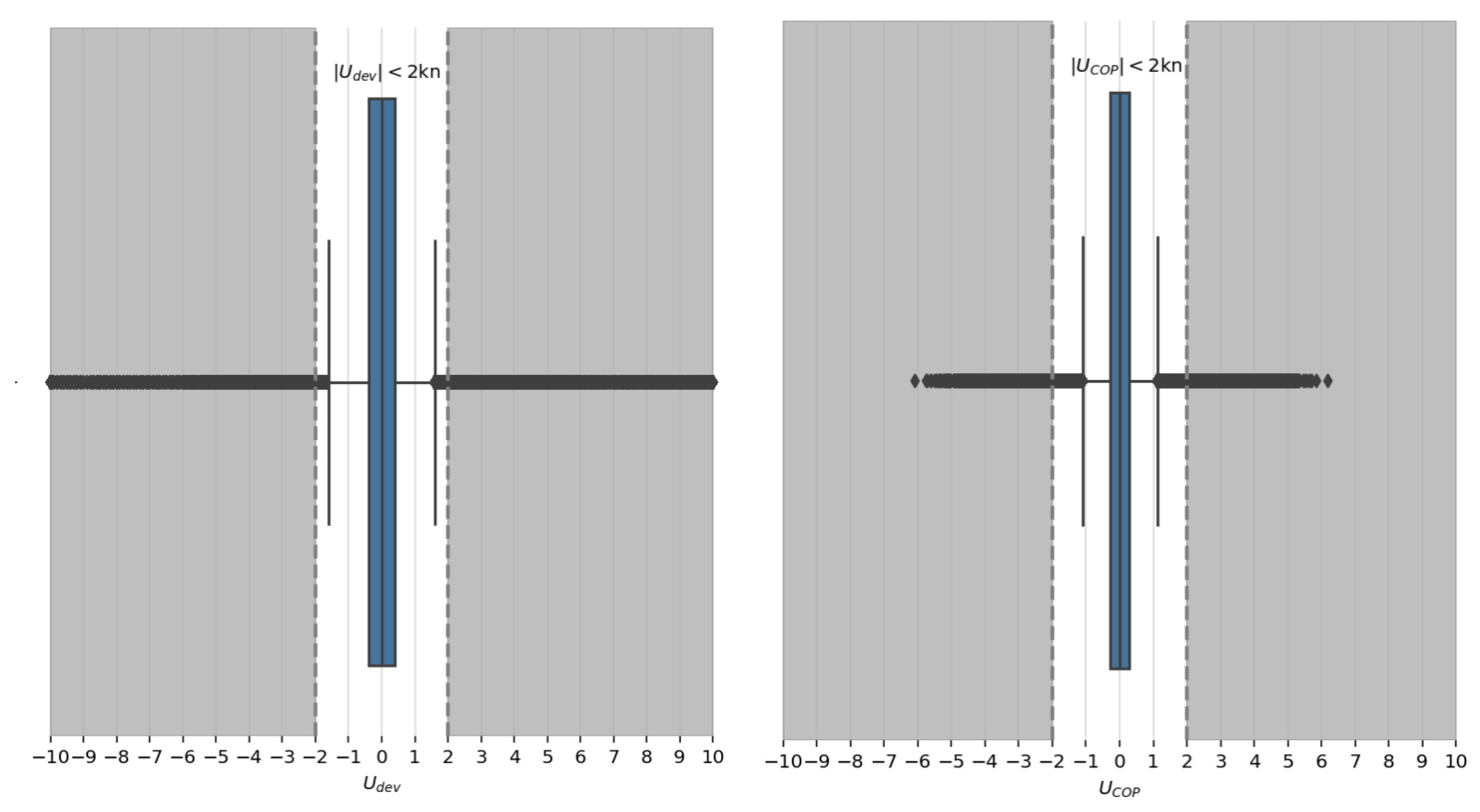
Speed deviation above and below 2 kn boundary.
Table 9.
Speed deviation above and below 2 kn boundary.
| | kn | kn | total |
|---|
| count | 7,152,295 | 181,195 | 7,333,490 |
| percentage% | % | % | 100% |
Table 10.
Speed deviation above 2 kn boundary decomposed by DVL manufacturer installed on the 190 ships of this study. Gray background occurs when kn percentage column is greater than .
Table 10.
Speed deviation above 2 kn boundary decomposed by DVL manufacturer installed on the 190 ships of this study. Gray background occurs when kn percentage column is greater than .
| Manufacturers | kn | Total |
|---|
| count | perc % |
|---|
| NaN | 52,000 | % | 1,947,949 |
| M.1 | 33,878 | % | 1,871,659 |
| M.2 | 32,254 | % | 1,325,151 |
| M.3 | 13,450 | % | 727,145 |
| M.4 | 11,068 | % | 618,358 |
| M.5 | 32,946 | % | 614,225 |
| M.6 | 5599 | % | 229,003 |
Table 11.
Speed deviation above 2 knots boundary decomposed by vessel class. Gray background shows up when kn percentage column is greater than and it gets darker while it increases.
Table 11.
Speed deviation above 2 knots boundary decomposed by vessel class. Gray background shows up when kn percentage column is greater than and it gets darker while it increases.
| Vessel Class | kn | Total |
|---|
| count | perc % |
|---|
| C.7 | 21,047 | % | 1,346,739 |
| C.26 | 24,727 | % | 1,251,124 |
| C.15 | 14,075 | % | 816,046 |
| C.9 | 7955 | % | 548,497 |
| C.16 | 19,651 | % | 559,411 |
| C.12 | 13,174 | % | 404,647 |
| C.10 | 12,024 | % | 338,794 |
| C.11 | 5293 | % | 285,827 |
| C.14 | 13,087 | % | 263,230 |
| C.24 | 2162 | % | 184,113 |
| C.27 | 943 | % | 180,521 |
| C.3 | 1784 | % | 161,798 |
| C.2 | 6500 | % | 137,575 |
| C.4 | 6834 | % | 132,552 |
| C.17 | 2300 | % | 117,575 |
| C.13 | 10,557 | % | 114,694 |
| C.21 | 1487 | % | 83,068 |
| C.5 | 991 | % | 69,454 |
| C.23 | 4641 | % | 70,161 |
| C.18 | 1468 | % | 62,934 |
| C.6 | 1145 | % | 59,429 |
| C.22 | 818 | % | 46,884 |
| C.1 | 499 | % | 40,939 |
| C.20 | 559 | % | 27,618 |
| C.25 | 55 | % | 11,745 |
| C.19 | 2705 | % | 13,401 |
| C.8 | 4714 | % | 4714 |
Table 12.
Speed deviation above 2 kn boundary decomposed by sea name where the ships have been sailing. Only those seas where the percentage column is greater than have been included. Gray background gets darker when the percentage column of kn increases.
Table 12.
Speed deviation above 2 kn boundary decomposed by sea name where the ships have been sailing. Only those seas where the percentage column is greater than have been included. Gray background gets darker when the percentage column of kn increases.
| Sea Region | kn | Total |
|---|
| count | perc % |
|---|
| North Atlantic Ocean | 30,656 | % | 913,938 |
| Indian Ocean | 29,353 | % | 839,133 |
| Arabian Sea | 9223 | % | 360,849 |
| North Sea | 6103 | % | 145,058 |
| English Channel | 14,413 | % | 84,719 |
| Japan Sea | 1764 | % | 55,680 |
| Alboran Sea | 2783 | % | 49,586 |
| Gulf of Mexico | 2040 | % | 33,947 |
| Andaman or Burma Sea | 1740 | % | 27,835 |
| Philippine Sea | 2710 | % | 19,548 |
| Gulf of St. Lawrence | 843 | % | 16,179 |
| Ionian Sea | 281 | % | 8840 |
| Strait of Gibraltar | 1925 | % | 7346 |
| Singapore Strait | 586 | % | 6648 |
| Coral Sea | 766 | % | 6104 |
| Rio de La Plata | 133 | % | 3633 |
| Tasman Sea | 468 | % | 3247 |
| Java Sea | 236 | % | 1647 |
| Arafura Sea | 150 | % | 1242 |
| Gulf of Thailand | 45 | % | 1228 |
| Great Australian Bight | 104 | % | 413 |
| Bass Strait | 35 | % | 247 |
Table 13.
Sea currents predicted speed above and below 2 kn boundary.
Table 13.
Sea currents predicted speed above and below 2 kn boundary.
| | kn | kn | Total |
|---|
| count | 7,287,465 | 46,025 | 7,333,490 |
| percentage% | % | % | 100% |
Table 14.
Sea surface currents speed projection on ship’s true heading above 2 kn boundary decomposed by sea name where the ships have been sailing. Only those seas where the percentage column is greater than have been included. Gray background gets darker when the percentage column of kn increases.
| Sea Region | kn | Total |
|---|
| count | perc % |
|---|
| North Atlantic Ocean | 6001 | % | 913,938 |
| Indian Ocean | 16,832 | % | 839,133 |
| South China Sea | 7769 | % | 539,339 |
| Malacca Strait | 2306 | % | 196,523 |
| North Sea | 2385 | % | 145,058 |
| English Channel | 2374 | % | 84,719 |
| Japan Sea | 818 | % | 55,680 |
| Gulf of Mexico | 595 | % | 33,947 |
| Philippine Sea | 1068 | % | 19,548 |
| Skagerrak | 265 | % | 17,745 |
| Strait of Gibraltar | 51 | % | 7346 |
| Singapore Strait | 135 | % | 6648 |
| Mozambique Channel | 11 | % | 1668 |
| Java Sea | 11 | % | 1647 |


 ,
, 


