


Abstract
We examined the dynamics of dinoflagellate cyst and phytoplankton assemblages in eutrophic coastal waters of Korea, adjacent to fish and shellfish farms. Water temperature showed seasonality, whereas salinity and pH remained relatively consistent. Dissolved inorganic nutrient levels were higher in September and at the inner stations, where aquaculture fish farms are located than those in May and at the outer stations. Canonical correspondence analysis and artificial neural network analysis revealed multiple environmental factors that affect the distribution of phytoplankton and dinoflagellate cysts. Diatoms dominated in the phytoplankton assemblages, while the protoperidinioid group dominated in the dinoflagellate cyst assemblages. Cyst abundance was higher at the outer stations than at the inner stations due to transport by fast currents, and phytoplankton abundance was positively correlated with cyst abundance. An increase in diatom abundance led to an increase in heterotrophic/mixotrophic cyst abundance, indicating that excessive uneaten food and urinary waste from the fish farms caused eutrophication in the study region and fast growth of diatoms, thereby contributing to the growth of heterotrophic/mixotrophic dinoflagellates and consequently, high abundance of heterotrophic/mixotrophic dinoflagellate cysts.
1. Introduction
Dinoflagellates are eukaryotic algae that produce resting cysts via sexual reproduction and/or temporary cysts in response to changes in environmental conditions such as temperature, salinity, and light [1]. The resting stage is a part of their life cycle, and the accumulated cysts can often resist harsh environmental conditions in sediments [2,3,4]; resting cysts play a pivotal role as seed populations, affecting phytoplankton communities during phytoplankton blooms [2,5,6,7]. Monitoring dinoflagellate cysts enables the temporal and spatial prediction of bloom initiation [2,8], tracking of historical records of harmful algal blooms [9], and analogy of historic environments in the water column and sediments [10].
As phytoplankton community structure varies with changes in environmental conditions and geographical characteristics of the study region and both species composition and abundance explicitly respond to physical and chemical conditions in the water column, phytoplankton are important for characterizing seawater environments [11]. For this reason, numerous previous studies have investigated how dinoflagellate cysts are associated with vegetative cells using environmental variables in coastal countries across the globe, including those in Asia [12,13,14,15,16,17], Europe [18,19,20,21], and North America [22,23,24].
Nutrients introduced from land via runoff contribute to high primary productivity in coastal waters, but excessive nutrient input exacerbates water quality and often causes harmful algal blooms [25,26]. Massive aquaculture farms are located along the southern coast of Korea; thus, organic matter originating from terrestrial regions and an excessive supply of food aggravate pollution around the aquaculture farms [27,28]. Typically, 40% of organic matter that flux into coastal sediments is degraded at the benthic boundary layer and 60% is buried in the aquaculture farm sediments [29]. Previous studies showed that a variety of organic matter from the aquaculture farms impacts the sediment and water column environments [30,31,32,33]. Therefore, to investigate the coastal region in which eutrophication driven by organic matter from aquaculture farms could cause algal blooms, the phytoplankton community in the water column and the dinoflagellate cyst community in modern sediments should be evaluated using environmental variables.
Studies on characterizing organic matter-driven pollution such as chemical fluxes of sediment boundary layers in fish farms [29] and the spatial and temporal distribution of nitrogen compounds [33] have been intensively performed, whereas the distribution of dinoflagellate cysts was only investigated once by Pospelova and Kim [34], who assessed the correlation of dinoflagellate cyst distribution with sediment environmental conditions. However, their study was confined to dinoflagellate cyst assemblages. Given that cysts are induced from vegetative cells in the water column, both the environmental conditions of the water column and surface sediments and the assemblages of phytoplankton and dinoflagellate cysts should be considered for investigating the spatial and temporal dynamics of dinoflagellate cysts. Therefore, in this study, we examined the spatial and temporal distribution of dinoflagellate cyst assemblages in surface sediments and phytoplankton assemblages in the water column, using the paleontological method and the microscopy method, respectively, focusing on how eutrophic water quality and sediment environments influence phytoplankton and dinoflagellate cyst distribution.
2. Materials and Methods
2.1. Study Region
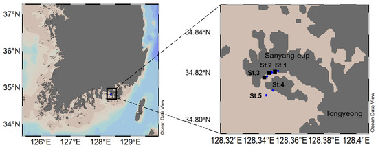
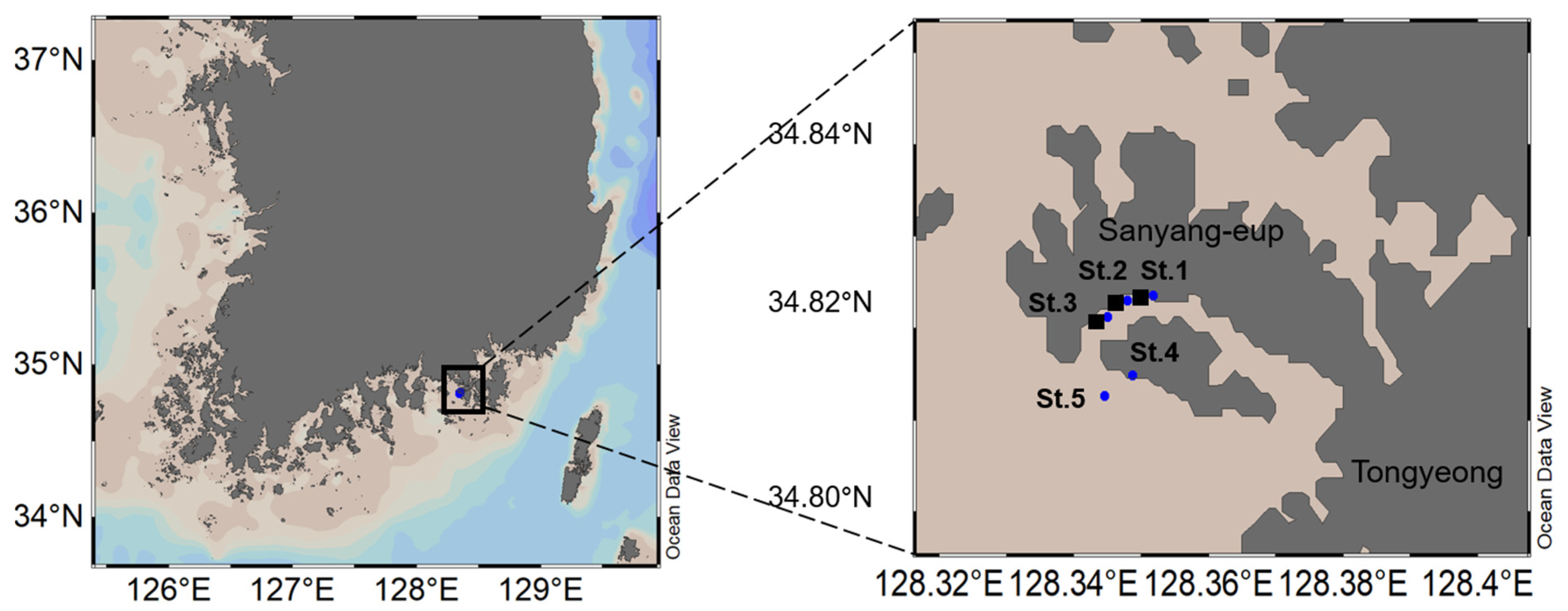
Tongyeong is located in Sanyang-eup in the Kyungsang-namdo province which is the central region of the southern coast of the Korean peninsula (39°49′ N, 128°21′ E; Figure 1), and its coastal waters surround the archipelago off the southern region of Korea. Various islands in this region are separated by muddy sediments, and frequent resuspension of sediments often causes high turbidity [35]. Aquaculture farms are overcrowded along the southern coastal waters of Korea. While there are no major rivers or streams that can contribute to the elevation of terrestrial nutrients, Tongyeong is representative of marine fish cages in the aquaculture industry and pollution driven from the marine fish cages has been aggravated [32]. This study region is shallow (<10 m depth) and characterized by the tidal currents flowing with a rate of 0.1~0.3 m/s depending on the locale [34]. The relatively slow tidal currents flow in the inner region and the tidal currents are relatively fast in the outer region of the study region [34].
Figure 1.
Map showing sampling stations in Tongyeong Sanyang-eup on the southern coast of Korea. Blue circles indicate sampling stations. Aquaculture fish farms were located near Stations 1–3, while no fish farms were deployed around Stations 4 and 5. Arrows indicate the direction of current movement in the study region. Blue circles are sampling stations and black squares denote the location of aquaculture fish cages.
2.2. Field Samples
Sampling was performed at five stations in two days in May and September 2006 with three inner stations (Stations 1, 2, and 3) and two outer stations (Stations 4 and 5; Figure 1). We collected samples for biotic (dinoflagellate cysts and phytoplankton) and abiotic samples (nutrients and sediment environments). Seawater samples were collected using a Niskin water sampler (General Oceanics, Miami, FL, USA) at 1 m below the water surface and 1 m above the bottom sediment; 1 L samples were fixed in polyethylene bottles with Lugol’s solution at a final concentration of 1%. The samples were covered with aluminum foil to inhibit fixative degradation by sunlight and were kept in a cooler with ice until the samples were delivered to the laboratory. Surface sediment samples were collected using a TFO gravity corer (University of Tokyo, Fisheries Oceanography Laboratory), consisting of a 30 cm-long and 1 cm-diameter tube. These tubes with 30 cm-long sediments were covered with aluminum foil to inhibit cyst germination by light and stored at 4 °C until further analyses. Subsequently, 20 mL nutrient samples were collected by filtering onto pre-combusted (2 h at 250 °C) glass fiber filters and stored in a −20 °C freezer until analysis. Physical and chemical parameters at the surface and bottom waters, including temperature, salinity, pH, and dissolved oxygen (DO), were measured on-site using a YSI 556 (YSI Inc., Yellow Springs, OH, USA).
2.3. Water and Sediment Sample Analysis for Environmental Variables
Ammonium, nitrate, nitrite, and phosphate were analyzed in duplicate using standard spectrophotometric methods [36,37,38]. Dissolved inorganic nitrogen (DIN) is defined as the summation of ammonium, nitrate, and nitrite. Water content was determined using the top 3 cm of sediments by calculating the ratio of the weight difference between the wet sediment and dried sediment (24 h at 110 °C) relative to the initial weight of the wet sediment. Sediment samples that were utilized to measure water content were also used to determine ignition loss (IL) by comparing the weight difference in the samples before and after combusting for 4 h at 550 °C. Generally, a direct measurement such as IL or organic carbon is utilized to estimate organic matter content in sediments [39], while chemical oxygen demand (COD) is utilized to quantify the amount of consumed oxygen during oxidation of organic matter [40]. COD was measured using the alkaline potassium permanganate method [41]. Acid volatile sulfide (AVS) is defined as the amount of hydrogen sulfide generated under anoxic conditions and is measured by converting sulfide in sediment to hydrogen sulfide [42]. To determine AVS, 2 g of sediment was transferred to a gas-generating tube and 2 mL of sulfuric acid (18N H2SO4) was added to measure the hydrogen sulfide using a gas detection tube.
The eutrophication index (E) is calculated to determine the degree of eutrophication in the study region. The index was calculated using COD and nutrients via derivation from a globally and locally applied equation, E = (COD × DIN × DIP)/3.43, where E is the eutrophication index, COD and DIN are as defined above, DIP is dissolved inorganic phosphate. When E > 1, the region is eutrophic and when E < 1, the region is not eutrophic [43,44].
2.4. Phytoplankton and Dinoflagellate Cyst Assemblage Analysis
Phytoplankton samples were transferred to settling tubes and settled for 48 h in the dark. The supernatant was then removed to yield 10 mL of concentrated samples [45]. Then, 1 mL of the final sample was mounted on a Sedgewick-Rafter counting chamber to quantify the phytoplankton assemblages using a light microscope (Olympus CH30; Olympus Corporation, Tokyo, Japan). Phytoplankton identification followed Shim [46] and Tomas [47].
Sample analysis for dinoflagellate cysts followed the paleontological method outlined in Matsuoka and Fukuyo [4]. The top 3 cm of the 30 cm-long sediment samples were weighed and then stored in the dark for 24 h after adding 15 mL of 10% hydrochloric acid to remove calcareous matter (e.g., foraminifera and fraction of shell). The acid-amended samples were washed multiple times using distilled water and stored in the dark after adding 15 mL of 47% fluoride acid to dissolve any siliceous matter (e.g., sand and diatom frustule). The samples were washed multiple times until the pH was 7 (i.e., samples turned neutral) and then transferred to 100 mL glass beakers to form a slurry. The samples were sonicated for 30 s and sieved using 125 µm and 20 µm sieves. Residual samples were transferred to 20 mL polyethylene tubes to create the final samples for cyst quantification. Finally, 1 mL samples were mounted on a Sedgewick-Rafter chamber to quantify the dinoflagellate cysts using an inverted microscope (AXIOVERT 200; Carl Zeiss AG, Oberkochen, Germany). The abundance of the dinoflagellate cysts was presented in terms of cysts/g dry as follows:
where N: total abundance of dinoflagellate cysts, W: weight of wet sediment (g), and R: ratio of sediment water content. N was obtained by multiplying the number of the counted cyst by 20, so that the number of cysts in 20 mL was calculated. Cyst identification followed Bolch and Hallegraeff [48], Nehring [8], and Matsuoka and Fukuyo [4].
cysts/g = N/W(1 − R)
2.5. Data Analysis and Statistical Analysis
To test the significant differences in the environmental variables between the surface water and bottom water and among stations, a Student t-test was performed on the water quality and sediment environmental variables, while the Kruskal–Wallis test was conducted to compare the DIN and DIP levels among the southern coastal waters of Korea. A Wilcoxon rank-sum test was utilized to compare the differences in the abundance of the biotic variables between May and September. A linear regression analysis was conducted on the cell abundance between the dinoflagellate cysts and phytoplankton to assess the relationship between two biological parameters. A canonical correspondence analysis (CCA) was performed to elucidate the relationship between the physicochemical variables of the seawater and phytoplankton assemblages and the environmental variables of the sediment and dinoflagellate cyst assemblages [27]. Statistical information of CCA from the phytoplankton and dinoflagellate cyst assemblages are presented in Tables S1 and S2, and the scree plot of each community is exhibited in Figures S1 and S2, respectively. An artificial neural network (ANN) model was assembled to evaluate the environmental variables with the most influence on the phytoplankton and dinoflagellate cyst abundance as a function of the water environmental variables and sediment environmental variables, respectively. A fundamental objective of recent ANN analysis tools including neuralnet [49], nnet [50], and RSNNS [51] is to address the concern that supervised neural networks are “black boxes” that provide no sufficient information about underlying relationships between variables [52,53]. The most popular form of neural network is the feed-forward multilayer perception trained using an error backpropagation training algorithm. The backpropagated error computed between the observed and estimated results is utilized to adjust the connection weights. This minimizes the error between the desired and predicted outputs [54,55]. The input data were transformed to a log form because the ranges of input data were wide. After the log-transformation, the dataset was scaled to a range from 0 to 1, prior to a train. ANN was operated predicting from weights and output data, while the modeled value was fed forward and compared to the measured response, from which the mean square error (MSE) was computed as 9.08 for phytoplankton and 6.84 for dinoflagellate cysts. 70% of data was utilized for training and 30% of data was utilized for validation. Measured environmental variables were considered as input neurons for ANN modeling processes, including temperature, salinity, pH, DO, DIN, and DIP for phytoplankton, and IL, AVS, COD, and water content for dinoflagellate cysts. ANN is usually applied to predict the response of one or more variables against one to many explanatory variables [56]. Thus, ANN is often used to elucidate the relative strength of environmental forces shaping phytoplankton biomass and community composition as a function of environmental variables [57,58,59,60]. A comparison test for the mean including a Student t-test, Kruskal–Wallis test, and Wilcoxon rank-sum test was performed using R (R Foundation for Statistical Computing, Vienna, Austria). The CCA was executed using XLSTAT (Addinsoft, Paris, France), and the ANN was accomplished using the package ‘neuralnet’ in R.
3. Results
3.1. Environmental Conditions in the Water Column
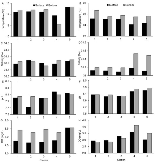
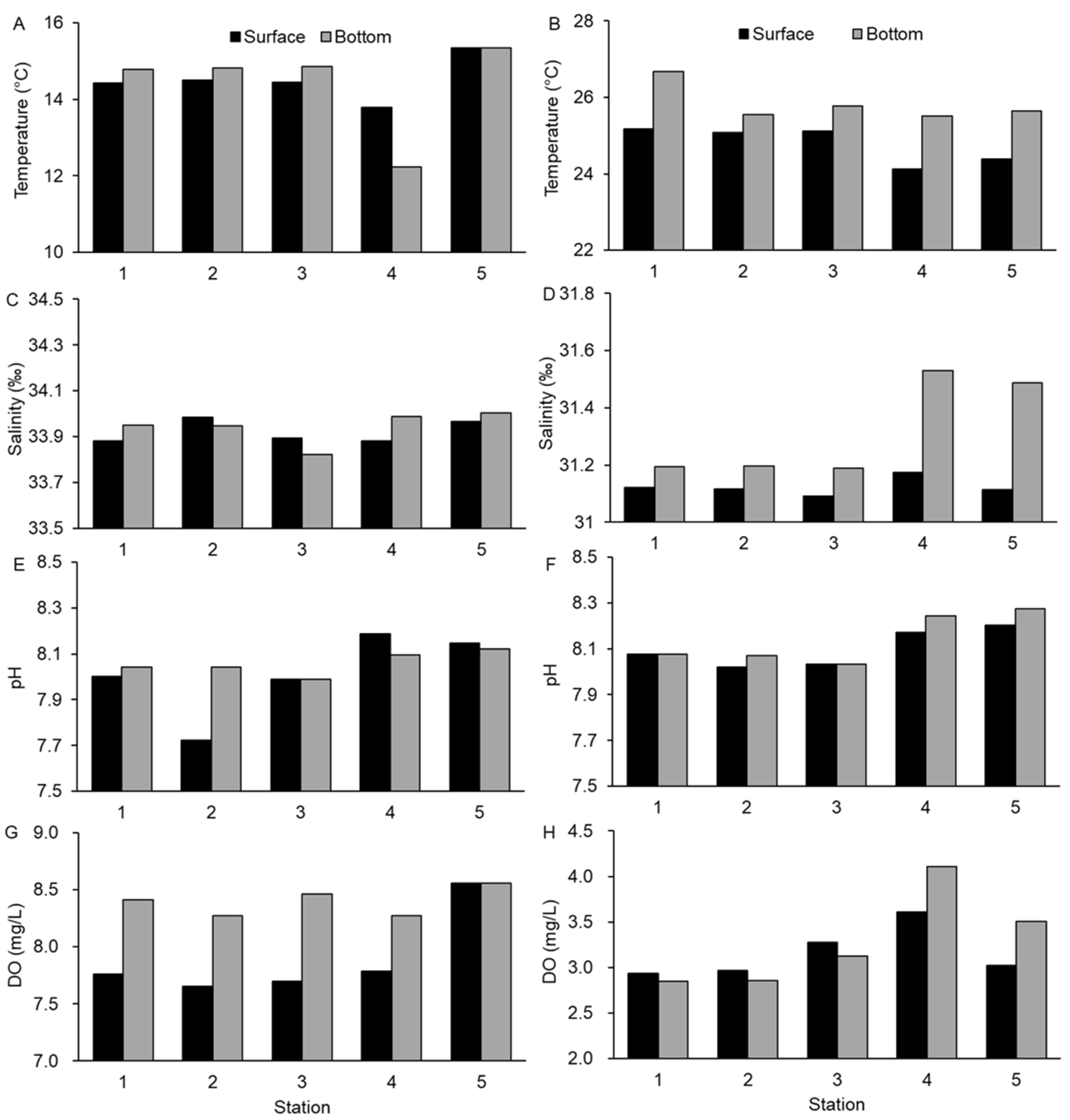
The environmental variables of the seawater slightly changed across the sampling stations (Figure 2). The temperature varied in the range 12.10–15.30 °C (mean ± standard deviation (sd): 14.30 ± 1.26 °C) in the surface water and 13.70–15.30 °C (14.44 ± 0.57 °C) in the bottom water in May (Figure 2A). Conversely, the water temperature increased to 25.27–26.65 °C (25.70 ± 0.55 °C) in the surface water and 24.00–25.14 °C (24.68 ± 0.56 °C) in the bottom water in September (Figure 2B). Salinity was fairly stable in May with 33.93 ± 0.08 psu at the surface and 33.90 ± 0.05 psu at the bottom (Figure 2C), whereas it was slightly lower in September at 31.13 ± 0.03 psu in the surface water and 31.33 ± 0.17 psu in the bottom water (Figure 2D). In September, the bottom salinity was slightly higher at the outer stations (Stations 4 and 5) than that at the inner stations (31.53 and 31.48 psu, respectively; Figure 2D). pH was not significantly different between the surface and bottom waters in May and September (p > 0.05; Student t-test), except at Station 2 in May (p < 0.05; Student t-test). However, pH at the inner stations, which were located close to the aquaculture fish farms, was slightly lower than that at the outer stations (Figure 2E,F). In May, DO in the bottom water (8.38 ± 0.13 mg/L) was significantly higher than that in the surface water (7.87 ± 0.39 mg/L; p < 0.05; Student t-test), except at 5 (Figure 2G). However, in September, the DO was fairly consistent between the surface and bottom waters at 3.26 ± 0.51 mg/L and 3.13 ± 0.30 mg/L, respectively (Figure 2H). DO at the outer stations was significantly higher than that at the inner stations (p < 0.05; Student t-test; Figure 2G,H).
Figure 2.
Water quality variables during the sampling period. (A) Water temperature (°C) in May, (B) Water temperature (°C) in September, (C) Salinity (‰) in May, (D) Salinity (‰) in September, (E) pH in May, (F) pH in September, (G) dissolved oxygen (DO; mg/L) in May, (H) DO (mg/L) in September. Circles denote water quality in the surface water, and squares denote water quality in the bottom water.
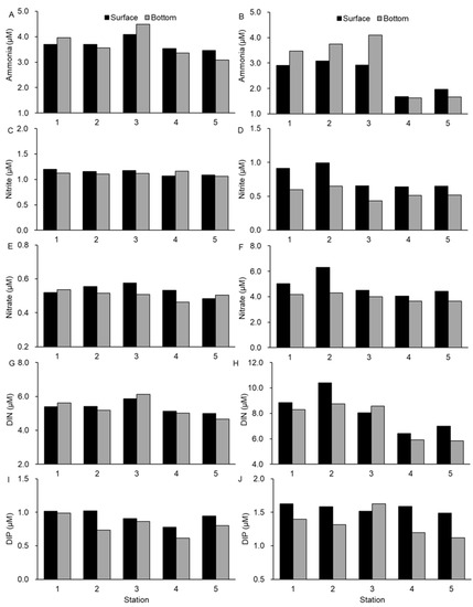
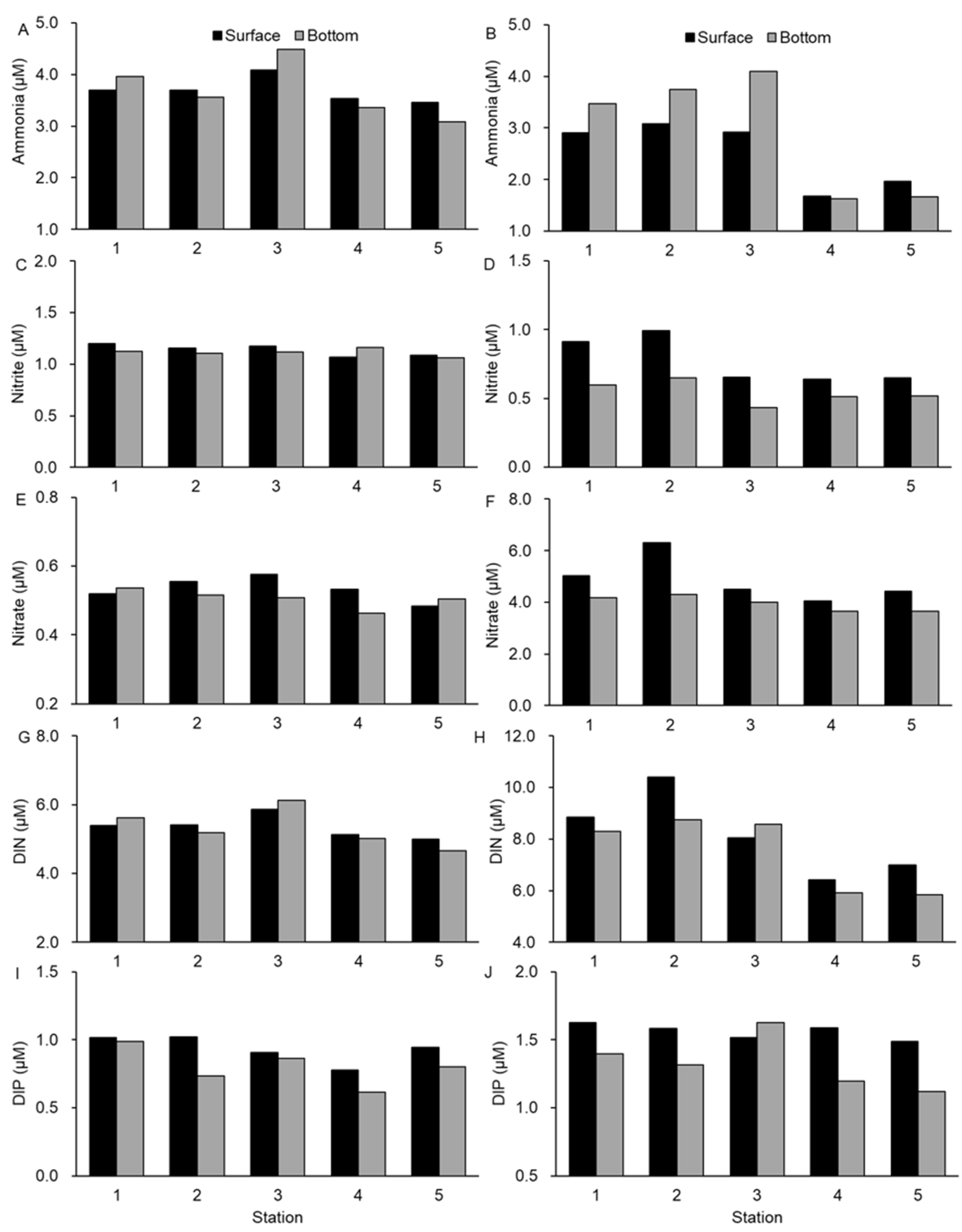
Generally, dissolved inorganic nutrient levels were lower at the outer stations than at the inner stations, while the differences between the surface and bottom waters in September were significantly higher (p < 0.05; Kruskal–Wallis test) compared to those in May (Figure 3). Ammonium levels varied in the range 3.07–4.49 µM (3.68 ± 0.55 µM) in the surface water, with 3.44–4.09 µM (3.69 ± 0.25 µM) in the bottom water in May (Figure 3A), but the levels were slightly lower in September, with a significant reduction at the outer stations (1.65 ± 0.02 µM) compared to those at the inner stations (3.77 ± 0.31 µM; p < 0.05; Kruskal–Wallis test; Figure 3B). Nitrite levels were relatively consistent in May and September (Figure 3C,D), but nitrate levels in the surface water and bottom water significantly increased from 0.51 ± 0.03 µM and 0.48 ± 0.57 µM in May to 3.99 ± 0.31 µM and 4.84 ± 0.86 µM in September, respectively (p < 0.05; Kruskal–Wallis test; Figure 3E,F). While the DIN levels in May were fairly stable among all stations, varying in the rage of 4.64–6.12 µM (5.30 ± 0.57 µM) in the surface water and 5.00–5.83 µM (5.34 ± 0.32 µM) in the bottom water (Figure 3G), the DIN levels in September significantly decreased from 9.09 ± 1.20 µM in the surface water and 8.54 ± 0.22 µM in the bottom water at the inner stations to 6.70 ± 0.41 µM in the surface water and 5.88 ± 0.04 µM in the bottom water at the outer stations (p < 0.05; Kruskal–Wallis test; Figure 3H). The DIP levels in May slightly decreased toward the outer stations with 0.79 ± 0.12 µM in the surface water and 0.92 ± 0.09 µM in the bottom water (Figure 3I). The decreasing pattern was similar in September, but the levels were moderately high with 1.33 ± 0.22 µM in the surface water and 1.55 ± 0.05 µM in the bottom water (Figure 3J).
Figure 3.
Dissolved inorganic nutrients (µM) in the study region. (A) Ammonia in May, (B) Ammonia in September, (C) Nitrite in May, (D) Nitrite in September, (E) Nitrate in May, (F) Nitrate in September, (G) Dissolved inorganic nitrogen (DIN; ammonia + nitrite + nitrate) in May, (H) DIN in September, (I) Dissolved inorganic phosphorous (DIP) in May, (J) DIP in September. Circles denote water quality in the surface water, and squares denote water quality in the bottom water.
3.2. Environmental Conditions in Sediments
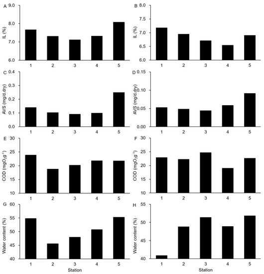
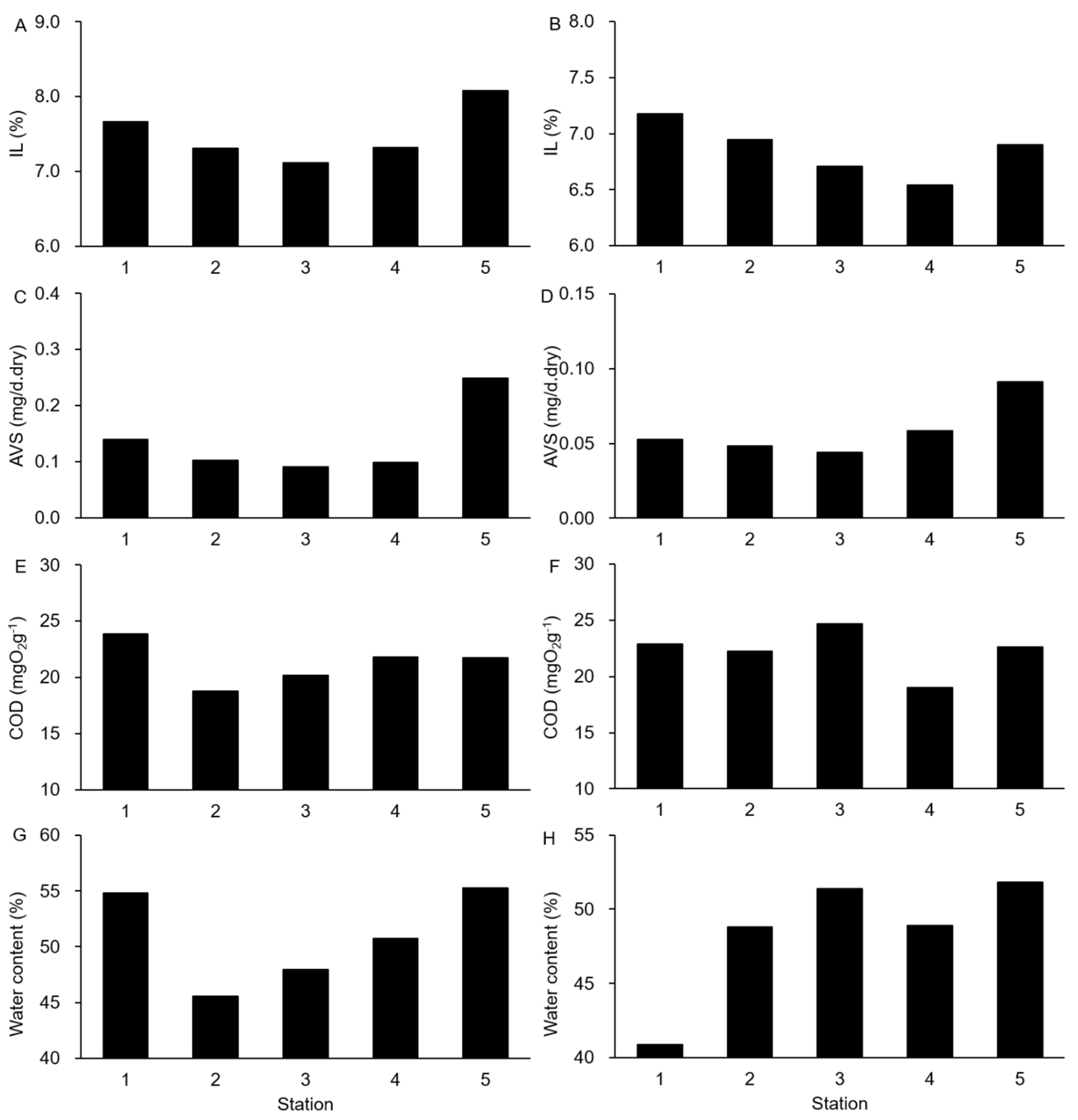
IL (%), AVS (mg/g dry), COD (mg O2/g), and water content (%) were measured to assess the environmental variation in the surface sediments (Figure 4). IL was stable at 7.07–8.11% (7.48 ± 0.41%) in May and 6.57–7.17% (6.88 ± 0.24%) in September (Figure 4A,B), whereas AVS sharply increased toward the outer stations with levels of 0.11 ± 0.03 mg/g dry at the inner stations and 0.17 ± 0.11 mg/g dry at the outer stations in May and 0.05 ± 0.00 mg/g dry at the inner stations and 0.07 ± 0.02 mg/g dry at the outer stations in September (Figure 4C,D). COD was not significantly different between May (21.16 ± 1.97 mg O2/g) and September (21.97 ± 1.96 mg O2/g; p > 0.05; Student t-test; Figure 4E,F). Water content varied among stations from 45.89% to 55.74% (51.27 ± 4.29%) in May and from 41.11% to 51.55% (48.47 ± 4.26%) in September (Figure 4G,H).
Figure 4.
Environmental variables of sediments in the study region. (A) Ignition loss (IL; %) in May, (B) IL in September, (C) Acid volatile sulfide (AVS; mg/g dry) in May, (D) AVS in September, (E) Chemical oxygen demand (COD; mg O2/g) in May, (F) COD in September, (G) Water content (%) in May, (H) Water content in September.
3.3. Characteristics of Phytoplankton Assemblages
A total of 20 genera and 32 species were observed in the phytoplankton in May, comprising 17 genera and 29 species of diatoms (91% of the total number of species), 2 genera and 2 species of dinoflagellates (6%), and 1 genus and 1 species of cryptophytes (3%; Table 1). Chaetoceros (10 species) was the most contributing genus, followed by Pseudo-nitzschia (3 species) and Thalassiosira (2 species) (Table 1). A larger variety of species were observed in September (41 genera and 70 species) than in May, with 27 genera and 50 species of diatoms (72%), 11 genera and 17 species of dinoflagellates (25%), and 1 genus and 1 species each of cryptophytes and euglenoids (1%; Table 2). Chaetoceros (13 species) was the most dominant genus, followed by Guinardia (4 species) and Prorocentrum (4 species; Table 2).
Table 1.
Phytoplankton assemblages in the surface and bottom waters in Tongyeong Sanyang-eup in May 2006 (×100 cells/L).
Table 2.
Phytoplankton assemblages in the surface and bottom waters in Tongyeong Sanyang-eup in September 2006 (×100 cells/L).
Phytoplankton abundance varied from 5.0 × 10⁵ to 11.3 × 10⁶ cells/L (mean of 7.7 × 10⁵ cells/L) in the surface water and from 2.2 × 10⁵ to 7.1 × 10⁵ cells/L (5.0 × 10⁵ cells/L) in the bottom water in May (Table 1). The abundance increased 10-fold in September, ranging from 8.5 × 10⁵ to 2.5 × 10⁶ cells/L in the surface water (1.6 × 10⁶ cells/L) and 8.7 × 10⁵ to 1.5 × 10⁶ cells/L in the bottom water (1.1 × 10⁶ cells/L; Table 2). The September abundance was significantly higher than the May abundance (p < 0.05; Wilcoxon rank-sum test; Table 1 and Table 2). The genus Chaetoceros dominated during the study period. In May, the most dominant species was Chaetoceros affinis (67.6%), and Chaetoceros didymus (6.6%) was subdominant, whereas in September, Chaetoceors curvisetus was the most dominant (25.1%), followed by Chaetoceros laciniosus, Chaetoceros compressus, and Chaetoceros didymus at 13.1%, 11.6%, and 10.2%, respectively (Table 1 and Table 2).
3.4. Characteristics of Dinoflagellate Cyst Assemblages
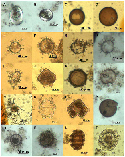
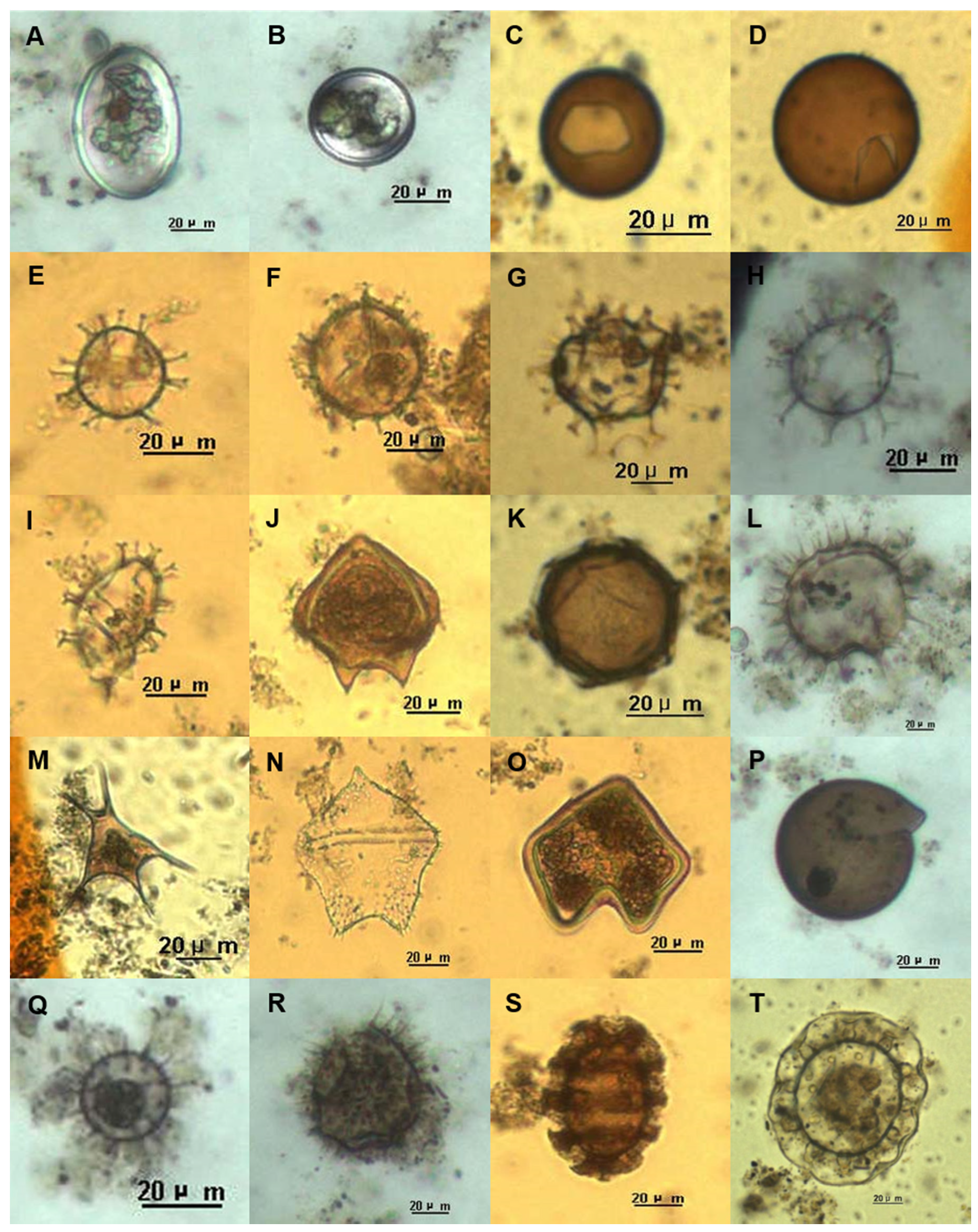
A total of 18 genera and 32 species were identified in the dinoflagellate cysts during the study period (Table 3; Figure 5). In May, 15 genera and 23 species were observed (Table 3), while the protoperidinioid group (7 genera and 11 species) had the greatest number of species with 48% of the dominance (Table 3). Furthermore, 2 genera and 6 species in the gonyaulacoid group (26%), 3 genera and 3 species in the gymnodinioid group (13%), 2 genera and 2 species in the diplopsalid group (9%), and 1 genus and 1 species of Tuberculodinium (4%) were identified (Table 3). The genus that contributed the most to the number of cyst species was Spiniferites (5 species), while Brigantedinium (3 species) and Protoperidinium (3 species) were subdominant (Table 3). A total of 17 genera and 28 species were identified in September. The protoperidinioid group (6 genera and 9 species) and the gonyaulacoid group (3 genera and 9 species) were the most dominant, with 32% dominance for each (Table 3). In addition, 4 genera and 5 species in the gymnodinioid group (18%), 2 genera and 2 species in the diplopsalid group (7%), 1 genus and 2 species in the calciodineloid group (7%), and 1 genus and 1 species of Tuberculodinium group were also identified (Table 3). The genera Spiniferites (5 species), Alexandrium (3 species), and Brigantedinium (3 species) were dominant (Table 3). Dinoflagellate cyst abundance increased from 3640–7380 cysts/g (mean of 4820 cysts/g) in May to 5140–9740 cysts/g (6340 cysts/g) in September (Table 3). Cyst abundance sharply increased at the outer stations (5960 ± 1980 cysts/g in May and 7480 ± 3200 cysts/g in September), while the abundance was 4040 ± 620 cysts/g in May and 5580 ± 560 cysts/g in September at the inner stations (Table 3). Particularly, the abundance was significantly higher at Station 5 than at the other stations (p < 0.05; Student t-test; Table 3). In May, Brigantedinium sp. was the most dominant species accounting for 24.4% of the dominance, while Spiniferites bulloideus, Brigantedinium caracoense, and the Polykrikos kofoidii/schwartzii complex followed with 23.7%, 11.4%, and 7.3% dominance, respectively (Table 3). In September, Brigantedinium sp. was still the most dominant with 21.8% dominance; additionally, Alexandrium affine (15.8%) and Spiniferites sp. (7.8%) were often identified (Table 3).
Table 3.
Dinoflagellate cyst assemblages in the surface sediments in Tongyeong Sanyang-eup in May and September 2006 (cysts/g).
Figure 5.
Photographs of dinoflagllate cysts found in the surface sediments adjacent from aquaculture fish farms in Tongyeong Snyang-eup, Southern coastal waters of Korea. (A). Alexandrium tamarense/catenella, (B). Alexandrium affine, (C). Brigantedinium caracoense, (D). Brigantedinium sp., (E). Spiniferites bulloides, (F). Spiniferites bentori, (G). Spiniferites membranaceus, (H). Spiniferites ramosus, (I). Spiniferites sp., (J). Quinquecuspis concretum, (K). Protoperidinium americanum, (L). Selenopemphix quanta, (M). Stelladinium reidii, (N). Trinovantedinium applanatum, (O). Votadinium carvum, (P). Gymnodinium catenatum, (Q). Oblea acantocysta, (R). Polykrikos hartmannii, (S). Polykrikos kofoiddi/schwartzii complex, (T). Tuberculodinium vacampoe.
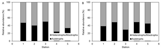
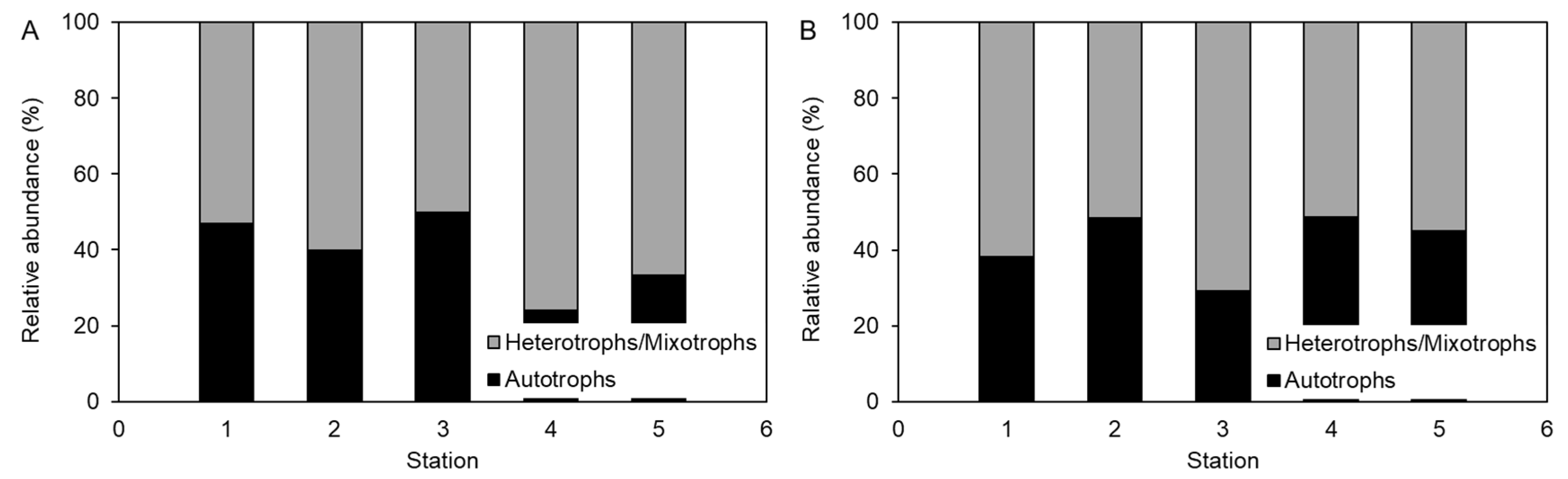
Dinoflagellate cysts were also quantified as either autotrophic or heterotrophic/mixotrophic species by trophic strategy (Table 3; Figure 6). In May, the abundance of autotrophic species ranged from 1080 to 2460 cysts/g (mean of 1820 cysts/g) with 38% dominance and the abundance of heterotrophic/mixotrophic species ranged from 1940 to 4900 cysts/g (2980 cysts/g) with 62% dominance (Table 3; Figure 6A). The relative abundance of heterotrophic/mixotrophic species was higher at Stations 4 and 5 than at the inner stations (Figure 6A). In September, the abundance of autotrophic species was between 1500 and 4360 cysts/g (2660 cysts/g), accounting for 42% of the total abundance, while the abundance of heterotrophic/mixotrophic species was between 2720 and 5380 cysts/g (3680 cysts/g) with 58% dominance (Table 3; Figure 6B). The relative abundance of heterotrophic/mixotrophic species at the outer stations was still higher (>50%) compared to that at the inner stations (Figure 6B). The ratio of autotrophic species to heterotrophic/mixotrophic species slightly decreased in September because more autotrophic species were identified, including the genus Scrippsiella in the calciodineloid group and the genus Alexandrium in the gonyaulacoid group (Table 3).
Figure 6.
Relative abundance of autotrophic and heterotrophic/mixotrophic cysts. (A) Relative abundance in May, (B) Relative abundance in September.
3.5. Relationship between Environmental Variables and Biotic Variables
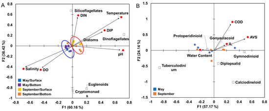
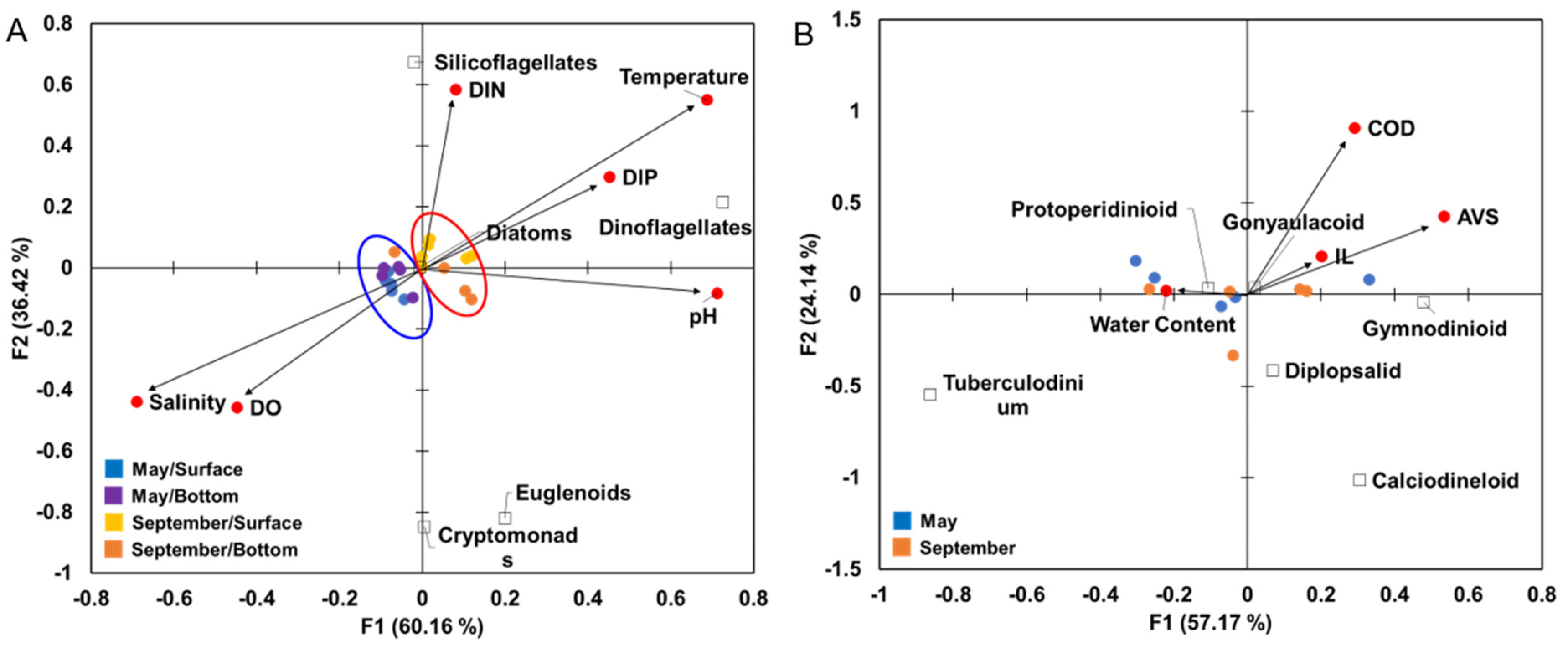
The CCA elucidated the relationship between the environmental variables and biotic variables (Figure 7). Phytoplankton assemblages were distinctively clustered by temperature and salinity, generating a clear segregation between the May and September populations (Figure 7A). The September phytoplankton communities exhibited a positive correlation with temperature and DIP, while the May communities presented a positive correlation with salinity and DO (Figure 7A). Particularly, diatoms and dinoflagellates were positively correlated with temperature and DIP (Figure 7A). In contrast to the phytoplankton assemblages, the CCA results for the dinoflagellate cyst assemblages showed no clear clusters between the two seasons, while COD and AVS were the most influential environmental variables on the dinoflagellate cyst communities (Figure 7B). The CCA revealed that the gonyaulacoid group was positively correlated with COD and AVS, while the protoperidinioid group was negatively correlated with COD and AVS but positively correlated with water content (Figure 7B).
Figure 7.
Ordination diagrams generated from the canonical correspondence analysis (CCA) illustrating the relationship between environmental variables and biotic variables during the study period. (A) CCA result for phytoplankton communities and water quality variables, (B) CCA result for dinoflagellate cyst communities and sediment environmental variables. Seasons and water depth are clarified by different colors. Phytoplankton samples were clustered into two groups by season, whereas cyst samples were randomly distributed on the CCA.
4. Discussion
4.1. Relationship between Water Quality and Phytoplankton Assemblages
Owing to a higher half-saturation constant (Km), diatoms require more nutrients than dinoflagellates, and diatom blooms succeed to dinoflagellate blooms when dissolved inorganic nutrients are limited [61,62,63,64]. After dissolved inorganic nutrients are excessively utilized by diatoms, dissolved organic nutrients (e.g., DON and DOP) become relatively high, and dinoflagellates that can utilize DON and DOP proliferate in coastal waters [65,66,67]. Although silicate was not measured, DIN and DIP levels can infer the growth of diatom populations. During the study period, the phytoplankton assemblages were mainly composed of diatoms and dinoflagellates; particularly, diatoms bloomed in September as a function of a sharp increase in nutrients from May to September. The DIN and DIP levels were significantly different (p < 0.05; Kruskal–Wallis test) between the inner stations located near the aquaculture fish cages and the outer stations connected to the open sea. This is because of the specific characteristics of the study region, where nitrogen and phosphorus compounds from aquaculture farms excessively contribute to the nutrient levels [35].
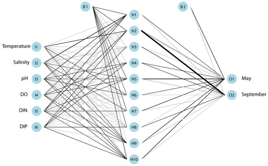
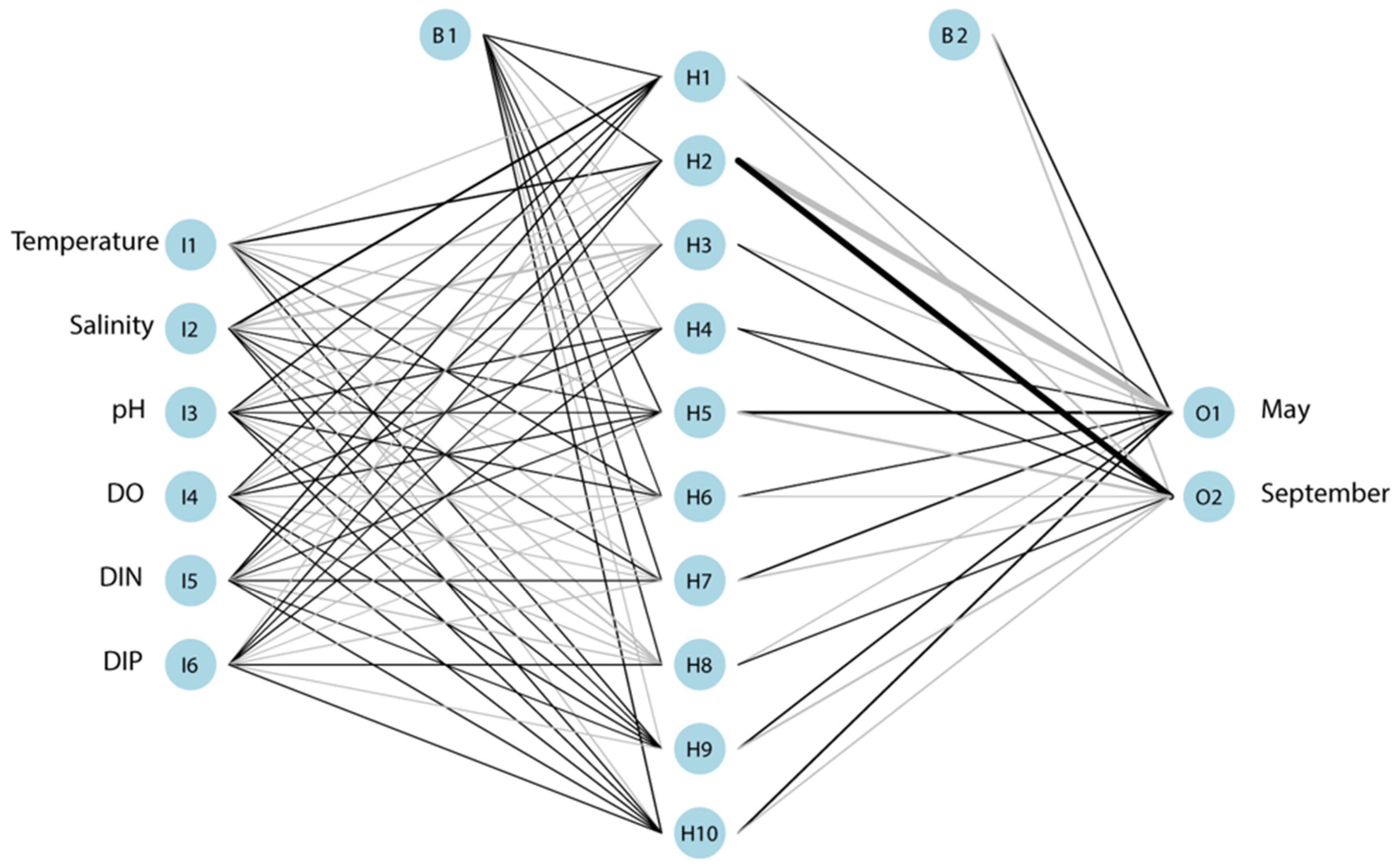
Multivariate analysis (e.g., CCA) showed the relationship between the environmental variables and phytoplankton assemblages; temperature, salinity, and DO were the most important environmental factors for phytoplankton communities. Consistent with these results, ANN for predicting phytoplankton abundance showed that, in May, the strength of the impact of DO and salinity was relatively large and positive while that of temperature was relatively large and negative (Figure 8). In September, as the water temperature increased above 20 °C, temperature and dissolved inorganic nutrients had a large positive strength of impact on phytoplankton abundance (Figure 8). This is because the increase in water temperature favored phytoplankton growth [68,69], and the decomposition rate of uneaten fish food and fish waste via bacterial activity became vigorous [70].
Figure 8.
Artificial neural network (ANN) for predicting phytoplankton abundance in May and September as a function of water environmental variables. The thickness of the lines joining the neurons is proportional to the strength of the connection weight. Black lines denote positive connections, and gray lines denote negative connections. One hidden layer was applied. Circles with B indicate additional inputs with layers, and bias are not affected by the previous layer.
Nutrients originating from aquaculture fish cages were characterized by dissolved and particulate matter. Dissolved nutrients are mostly composed of nitrogen and therefore cause coastal eutrophication because 60% of the released nitrogen is dissolved in the water column. Meanwhile, excessive food and fish waste that are released in the form of particulate matter settle in the surface sediments and are moved to adjacent waters by currents [71]. Only a part of the phosphorus in fish food is assimilated to the fish body and most of the assimilated phosphorus is defecated as fish waste, leading to coastal eutrophication. According to Ackefors and Enell [72], 30% of phosphorous released from uneaten food returned to the fish body by assimilation, and 54% and 16% of the released P compounds are excreted in the form of particulate and dissolved matter, respectively. Eutrophication index (E) was greater than 1 across the sampling stations, an indicator of eutrophication [43,44] and E significantly increased in September as temperature increased (p < 0.05; Kruskal–Wallis test; Table 4). In addition, the DIN and DIP levels in the study region were higher compared to those in the adjacent coastal waters, indicating that the seawater around the Tongyeong fish farms is more eutrophic than other regions along the southern coastal waters of Korea (p < 0.05; Kruskal–Wallis test; Table 5). The DIP levels in the study region were more than twice those in the adjacent coastal waters both in May (p < 0.05) and September (p < 0.01; Kruskal-Wallis test; Table 5); the DIN levels in the study region were significantly higher than those in the other southern coastal waters (p < 0.05; Kruskal–Wallis test; Table 5), indicating that the N and P compounds excreted from the excessive fish food and the fecal and urinary products exacerbated the water quality of the study region.
Table 4.
Eutrophication index (E) in Tongyeong Sanyang-eup during the study period. The index was calculated as E = (COD × DIN × DIP)/3.43, where COD is chemical oxygen demand, DIN is dissolved inorganic nitrogen, and DIP is dissolved inorganic phosphate [43,44].
Table 5.
Comparison of dissolved inorganic nutrient levels around the southern coastal waters of Korea. Asterisk indicates a significantly different level from other regions (* p < 0.05, ** p < 0.01; Kruskal–Wallis test). DIN, dissolved inorganic nitrogen; DIP, dissolved inorganic phosphorus.
4.2. Relationship between Sediment Environments and Dinoflagellate Cyst Assemblages in Eutrophic Sediments
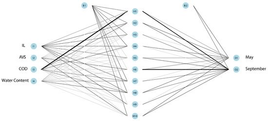
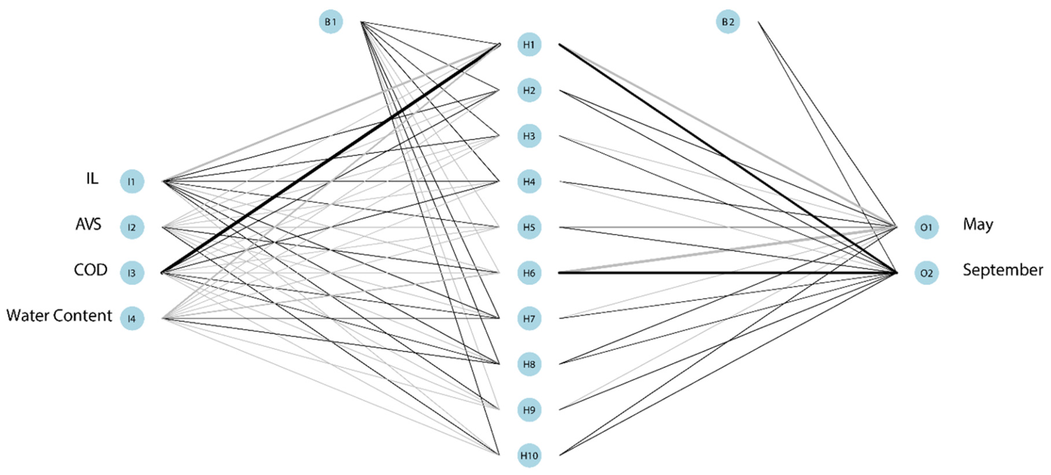
The extent of eutrophication determines the patterns of organic matter distribution, and the levels of organic matter outstand the southeastern coast of Korea from the Jinju Bay to the Yeongil Bay [73]. The COD levels in the sediments of the fish farms in Tongyeong Sanyang-eup are above the standard level of 20 mg O2/g dry [74], indicating that sediment eutrophication in the study region has proceeded due to the massive fish farms and input of sewage and livestock waste from land. The ANN for predicting dinoflagellate cyst abundance also illustrated the strength of the impact of sediment environmental variables on cyst abundance. Largely, COD was the most influential sediment environmental variable while AVS also positively affected cyst abundance in September (Figure 9). In addition, the ratio of COD to IL (COD/IL) can be utilized to determine the origin of organic matter and the characteristics of sediment distribution, with the organic matter being allochthonous when COD/IL > 1 and autochthonous when COD/IL <1 [64]. The relatively high COD/IL ratios in the study region (2.83 ± 0.23 in May and 3.19 ± 0.28 in September; Table S3) suggest that the organic matter in the sediments is not likely to have originated from marine aquatic organisms but rather from anthropogenic input such as wastes from fish farms.
Figure 9.
Artificial neural network (ANN) for predicting dinoflagellate cyst abundance in May and September as a function of sediment environmental variables. The thickness of the lines joining the neurons is proportional to the strength of the connection weight. Black lines denote positive connections, and gray lines denote negative connections. One hidden layer was applied. Circles with B indicate additional inputs with layers, and bias are not affected by the previous layer.
In the eutrophic water, heterotrophic/mixotrophic cysts have been detected more than autotrophic cysts, with a high ratio of heterotrophic/mixotrophic species to autotrophic species [16,19,75,76]. In accordance with this, the abundance of heterotrophic/mixotrophic cysts was higher than that of autotrophic cysts across all stations in our study, constituting 62% and 58% of total dinoflagellate cysts in May and September, respectively, inferring that eutrophication has been worsened due to the input of organic matter from the fish farms. Previous studies revealed that the number of species and abundance of dinoflagellate cysts in the eutrophic sediments are higher than those in non-eutrophic sediments [20,77], which is consistent with previous study results from coastal sediments in Korea [14,15,78,79,80]. While 18 genera and 32 species were identified in this study, previous studies have shown that the number of dinoflagellate cysts in the southern coastal sediments of Korea includes 2 genera and 27 species in the Jinhae Bay [78], 17 genera, and 30 species in the Gwangyang Bay [15], and 19 genera and 30 species in Geoje [81].
Generally, total cyst abundance in the study region was relatively high and the abundance sharply increased at the outer stations (4820 ± 100 cysts/g at the inner stations vs. 6720 ± 220 cysts/g at the outer stations). As previously mentioned, currents move organic matter originating from aquaculture fish farms to adjacent waters [71]. The fish farms in Tongyeong are employed in coastal waters with fast currents due to the efficient removal of the excessive organic matter [33]. As currents relocated organic matter, dinoflagellate cysts in the surface sediments were also transferred in the direction of the current movement; therefore, cysts accumulated at the outer stations, resulting in higher cyst abundance.
Interestingly, the genus Alexandrium was identified in the study region in September, including Alexandrium affine and Alexandrium catenella/pacificum (Alexandrium pacificum = formerly Alexandrium tamarense). The detection level of paralytic shellfish poisoning (PSP) toxins caused by Alexandrium blooms has already exceeded the federal closure limit in this region, and closure of the harvest bay annually occurs in May [82]. Recently, the extent of the toxin level has aggravated [83], and the PSP toxins also caused human deaths in the 1980s and 1990s in Geoje and Busan, Korea [82,84]. The occurrence of favorable conditions for cyst germination enables red tides, which drive fish mortality in aquaculture farms and further threaten the health of human beings [85]. Given that a moderate abundance of Alexandrium cysts appeared in the study region and cysts can play a role as seed populations for blooms [86], continuous monitoring is necessary to detect red tides caused by Alexandrium species.
4.3. Relationship between Phytoplankton and Dinoflagellate Cysts
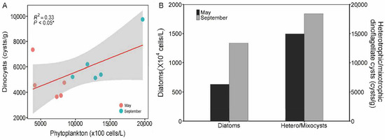
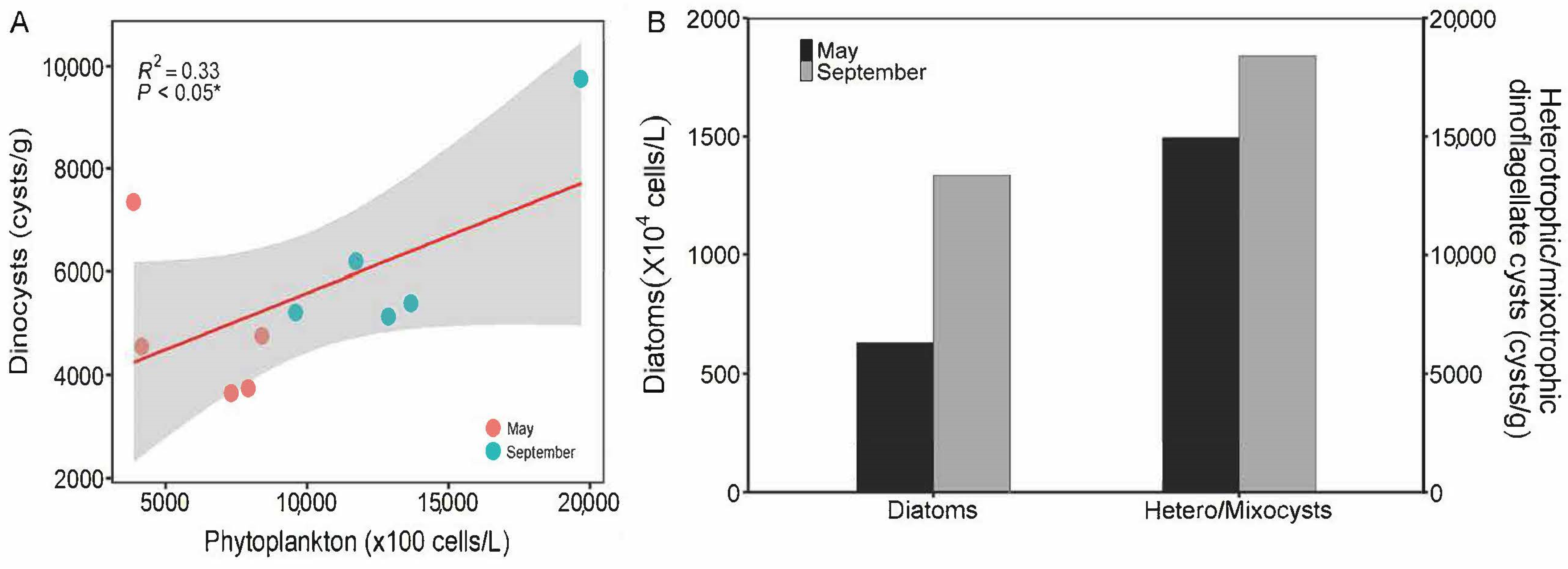
Heterotrophic/mixotrophic dinoflagellates utilize diatoms as a food source for growth [87,88,89]. Protoperidinium species of heterotrophic dinoflagellates feed on a variety of diatoms during diatom blooms or take up excreted dissolved/decaying organic matter from diatoms after the blooms [90,91]. Gaines and Taylor [87] and Jacobson and Anderson [88] described a feeding mechanism in which heterotrophic dinoflagellates deploy pseudopods to completely surround relatively large diatoms and then dissolve their cell contents. In concert with the feeding behavior of heterotrophic dinoflagellates, the seasonal abundance of heterotrophic/mixotrophic dinoflagellate cysts is positively proportional to diatom abundance, which was determined using a sediment trap in a prior study [92]. For this reason, heterotrophic/mixotrophic dinoflagellate cysts are associated with the abundance of diatoms, while heterotrophic/mixotrophic cysts dominate in highly productive regions such as upwelling regions [93,94,95]. Consistent with this, our study showed a positive correlation of dinoflagellate cysts with phytoplankton abundance (R2 = 0.33; p < 0.05; linear regression; Figure 10A), and consequently, the abundance of heterotrophic/mixotrophic dinoflagellate cysts significantly increased in September in accordance with a significant increase in diatom abundance (Figure 10B). This is because the intrusion of excessive nutrients from aquaculture farms and higher temperature led to the fast growth of diatoms in the warm season (September) and then drove the formation of more heterotrophic/mixotrophic dinoflagellate cysts in the modern sediments. The vertical profile of the dinoflagellate cysts in the study region was not investigated; however, the long history of aquaculture farms in the study region (>30 years) suggests that a long-term process of eutrophication might also have resulted in a relatively high abundance of heterotrophic/mixotrophic dinoflagellates in the past, and a general link between diatoms and heterotrophic/mixotrophic dinoflagellate cysts in relatively recent sediments in the study region.
Figure 10.
Relationship between phytoplankton abundance and dinoflagellate cyst abundance. (A) Linear regression of phytoplankton abundance and dinoflagellate cyst abundance in the study region in May and September. Red indicates abundance in May, and blue indicates abundance in September. The abundance of phytoplankton and cysts in September was significantly higher than that in May (Wilcoxon rank-sum test; p < 0.05). As phytoplankton abundance increased from September to May, dinoflagellate cyst abundance also increased proportionally. (B) Comparison of diatom and heterotrophic/mixotrophic cyst abundance in May and September. A Wilcoxon rank-sum test was performed to compare the difference in abundance between May and September (p < 0.001 for diatoms, p < 0.5 for heterotrophic/mixotrophic dinoflagellate cysts). Hetorocyst = heterotrophic/mixotrophic dinoflagellate cysts.
Supplementary Materials
The following are available online at https://www.mdpi.com/article/10.3390/jmse9040362/s1, Table S1: Statistical information of canonical correspondence analysis on phytoplankton assemblages, Table S2: Statistical information of canonical correspondence analysis on dinoflagellate cyst assemblages, Figure S1: Scree plot from canonical correspondence analysis on phytoplankton assemblages, Figure S2: Scree plot from canonical correspondence analysis on dinoflagellate cyst assemblages, Table S3 Environmental variables of the surface sediments in Tongyeong Sanyang-eup in May and September 2006 (mean ± standard deviation).
Author Contributions
Conceptualization, Y.K. and C.-H.M.; investigation, data curation, writing—original draft preparation, Y.K.; writing—review and editing, H.-J.K.; funding acquisition, Y.K. and C.-H.M. All authors have read and agreed to the published version of the manuscript.
Funding
This study was supported by a grant of Basic Science Research Program through the National Research Foundation of Korea funded by the Ministry of Education, Science and Technology (No. 2020R1F1A1076628).
Institutional Review Board Statement
Not applicable.
Informed Consent Statement
Not applicable.
Acknowledgments
We appreciate researchers and students at the Department of Oceanography of Pukyong National University who assisted with sampling data analysis.
Conflicts of Interest
The authors declare that they have no known competing financial interests or personal relationships that could have appeared to influence the work reported in this paper.
References
- Dale, B. Dinoflagellate resting cysts: “Benthic plankton”. In Survival Strategies of the Algae; Fryxell, G.A., Ed.; Cambridge University Press: Cambridge, UK, 1983; p. 144. [Google Scholar]
- Anderson, D.M.; Wall, D. Potential importance of benthic cysts of Gonyaulax tamarensis and G. excavata in initiating toxic dinoflagellate blooms. J. Phycol. 1978, 14, 224–234. [Google Scholar] [CrossRef] [Scilit]
- Hallegraeff, G.M.; Bolch, C.J. Transport of toxic dinoflagellate cysts via ships’ ballast water. Mar. Pollut. Bull. 1991, 22, 27–30. [Google Scholar] [CrossRef] [Scilit]
- Matsuoka, K.; Fukuyo, Y. Technical Guide for Modern Dinoflagellate Cyst Study; WESTPAC-HAB, Japan Society for the Promotion of Science: Tokyo, Japan, 2000. [Google Scholar]
- Anderson, D.M.; Coats, D.W.; Tyler, M.A. Encystment of the dinoflagellate Gyrodinium uncatenum: Temperature and nutrient effects. J. Phycol. 1985, 21, 200–206. [Google Scholar] [CrossRef] [Scilit]
- Balch, W.M.; Reid, P.C.; Surrey-Gent, S.C. Spatial and temporal variability of dinoflagellate cyst abundance in a tidal estuary. Can. J. Fish. Aquat. Sci. 1983, 40, s244–s261. [Google Scholar] [CrossRef] [Scilit]
- Kim, Y.-O.; Park, M.-H.; Han, M.-S. Role of cyst germination in the bloom initiation of Alexandrium tamarense (Dinophyceae) in Masan Bay, Korea. Aquat. Microb. Ecol. 2002, 29, 279–286. [Google Scholar] [CrossRef] [Scilit]
- Nehring, S. Dinoflagellate resting cysts from recent German coastal sediments. Bot. Mar. 1997, 40, 307–324. [Google Scholar] [CrossRef] [Scilit]
- Cho, H.-J.; Lee, J.-B.; Moon, C.-H. Dinoflagellate cyst distribution in the surface sediments from the East China sea around Jeju Island. Korean J. Environ. Biol. 2004, 22, 192–199. [Google Scholar]
- Zonneveld, K.A.; Bockelmann, F.; Holzwarth, U. Selective preservation of organic-walled dinoflagellate cysts as a tool to quantify past net primary production and bottom water oxygen concentrations. Mar. Geol. 2007, 237, 109–126. [Google Scholar] [CrossRef] [Scilit]
- Smayda, T. Biogeographical meaning; indicators. In Phytoplankton Manual; Sournia, A., Ed.; UNESCO: Paris, France, 1978; pp. 225–229. [Google Scholar]
- Matsuoka, K.; Kawami, H.; Nagai, S.; Iwataki, M.; Takayama, H. Re-examination of cyst–motile relationships of Polykrikos kofoidii and Polykrikos schwartzii Bütschli (Gymnodiniales, Dinophyceae). Rev. Palaeobot. Palynol. 2009, 154, 79–90. [Google Scholar] [CrossRef] [Scilit]
- Matsuoka, K.; Mizuno, A.; Iwataki, M.; Takano, Y.; Yamatogi, T.; Yoon, Y.H.; Lee, J.-B. Seed populations of a harmful unarmored dinoflagellate Cochlodinium polykrikoides Margalef in the East China Sea. Harmful Algae 2010, 9, 548–556. [Google Scholar] [CrossRef] [Scilit]
- Kang, Y.J.; Ko, T.H.; Lee, J.A.; Lee, J.-B.; Chung, I.K. The community dynamics of phytoplankton and distribution of dinoflagellate cysts in Tongyoung Bay, Korea. Algae 1999, 14, 43–54. [Google Scholar]
- Kim, S.-Y.; Moon, C.-H.; Cho, H.-J.; Lim, D.-I. Dinoflagellate cysts in coastal sediments as indicators of eutrophication: A case of Gwangyang Bay, South Sea of Korea. Estuaries Coasts 2009, 32, 1225–1233. [Google Scholar] [CrossRef] [Scilit]
- Kim, H.-J.; Moon, C.-H.; Cho, H.-J. Spatial-temporal characteristics of dinoflagellate cyst distribution in sediments of Busan Harbor. Sea 2005, 10, 196–203. [Google Scholar]
- Xiao, Y.-Z.; Wang, Z.-H.; Chen, J.-F.; Lu, S.-H.; Qi, Y.-Z. Seasonal dynamics of dinoflagellate cysts in sediments from Daya bay, the south China sea its Relation to the bloom of Scrippsiella trochoidea. Acta Hydrobiol. Sin. 2003, 27, 377–383. [Google Scholar]
- Nehring, S. Dinoflagellate resting cysts as factors in phytoplankton ecology of the North Sea. Helgol. Meeresun 1995, 49, 375–392. [Google Scholar] [CrossRef] [Scilit]
- Dale, B. The sedimentary record of dinoflagellate cysts: Looking back into the future of phytoplankton blooms. Sci. Mar. 2001, 65, 257–272. [Google Scholar] [CrossRef] [Scilit]
- Nehring, S. Scrippsiella spp. resting cysts from the German bight (North Sea): A tool for more complete check-lists of dinoflagellates. Neth. J. Sea Res. 1994, 33, 57–63. [Google Scholar] [CrossRef] [Scilit]
- Zonneveld, K.A.; Dale, B. The cyst-motile stage relationships of Protoperidinium monospinum (Paulsen) Zonneveld et Dale comb. nov. and Gonyaulax verior (Dinophyta, Dinophyceae) from the Oslo Fjord (Norway). Phycologia 1994, 33, 359–368. [Google Scholar] [CrossRef] [Scilit]
- Radi, T.; Pospelova, V.; de Vernal, A.; Vaughn Barrie, J. Dinoflagellate cysts as indicators of water quality and productivity in British Columbia estuarine environments. Mar. Micropaleontol. 2007, 62, 269–297. [Google Scholar] [CrossRef] [Scilit]
- Anglès, S.; Garcés, E.; Hattenrath-Lehmann, T.K.; Gobler, C.J. In situ life-cycle stages of Alexandrium fundyense during bloom development in Northport Harbor (New York, USA). Harmful Algae 2012, 16, 20–26. [Google Scholar] [CrossRef] [Scilit]
- Cremer, H.; Sangiorgi, F.; Wagner-Cremer, F.; McGee, V.; Lotter, A.F.; Visscher, H. Diatoms (Bacillariophyceae) and dinoflagellate cysts (Dinophyceae) from Rookery bay, Florida, USA. Caribb. J. Sci. 2007, 43, 23–58. [Google Scholar] [CrossRef] [Scilit]
- Anderson, D.M.; Burkholder, J.M.; Cochlan, W.P.; Glibert, P.M.; Gobler, C.J.; Heil, C.A.; Kudela, R.M.; Parsons, M.L.; Rensel, J.E.J.; Townsend, D.W.; et al. Harmful algal blooms and eutrophication: Examining linkages from selected coastal regions of the United States. Harmful Algae 2008, 8, 39–53. [Google Scholar] [CrossRef] [Scilit]
- Glibert, P.M.; Al-Azri, A.; Icarus Allen, J.; Bouwman, A.F.; Beusen, A.H.; Burford, M.A.; Harrison, P.J.; Zhou, M. Key questions and recent research advances on harmful algal blooms in relation to nutrients and eutrophication. Glob. Ecol. Oceanogr. Harmful Algal Bloom. 2018, 232, 229–259. [Google Scholar]
- Kang, Y.; Kang, H.-Y.; Kim, D.; Lee, Y.-J.; Kim, T.-I.; Kang, C.-K. Temperature-dependent bifurcated seasonal shift of phytoplankton community composition in the coastal water off southwestern Korea. Ocean Sci. J. 2019, 54, 467–486. [Google Scholar] [CrossRef] [Scilit]
- Kim, B.; Choi, A.; Kim, H.C.; Jung, R.H.; Lee, W.C.; Hyun, J.H. Rate of sulfate reduction an diron reduction in the sediment associated with ablone aquaculture in the southern coastal wateres of Korea. Ocean Polar Res. 2011, 33, 435–445. [Google Scholar] [CrossRef] [Scilit]
- Shim, J.-H.; Kang, Y.-C.; Choi, J.-W. Chemical fluxes at the sediment-water interface below marine fish cages on the coastal waters off Tong-Young, South Coast of Korea. J. Korean Soc. Oceanogr. 1997, 2, 151–159. [Google Scholar]
- Ritz, D.; Lewis, M.; Shen, M. Response to organic enrichment of infaunal macrobenthic communities under salmonid seacages. Mar. Biol. 1989, 103, 211–214. [Google Scholar] [CrossRef] [Scilit]
- Pearson, T.; Rosenberg, R. Macrobenthic succession in relation to organic enrichment and pollution of the marine environment. Oceanogr. Mar. Biol. Annu. Rev. 1978, 16, 229–311. [Google Scholar]
- Park, H.-S.; Choi, J.-W.; Lee, H.-G. Community structure of macrobenthic fauna under marine fish culture cages near Tongyong, Southern Coast of Korea. Korean J. Fish. Aquat. Sci. 2000, 33, 1–8. [Google Scholar]
- Jang, Y.L.; Lee, H.J.; Moon, H.-B.; Lee, W.-C.; Kim, H.C.; Kim, G.B. Marine environmental characteristics in the coastal area surrounding Tongyeong cage-fish farms. J. Korean Soc. Mar. Environ. Energy 2015, 18, 74–80. [Google Scholar] [CrossRef] [Scilit]
- Pospelova, V.; Kim, S.-J. Dinoflagellate cysts in recent estuarine sediments from aquaculture sites of southern South Korea. Mar. Micropaleontol. 2010, 76, 37–51. [Google Scholar] [CrossRef] [Scilit]
- Lee, Y.S.; Lim, W.A.; Jung, C.S.; Park, J. Spatial distributions and monthly variations of water quality in coastal seawater of Tongyeong, Korea. J. Korean Soc. Mar. Environ. Eng. 2011, 14, 154–162. [Google Scholar] [CrossRef] [Scilit]
- Jones, M.N. Nitrate reduction by shaking with cadmium—Alternative to cadmium columns. Water Res. 1984, 18, 643–646. [Google Scholar] [CrossRef] [Scilit]
- Parsons, T.R.; Maita, Y.; Lalli, C.M. A Manual of Chemical and Biological Methods for Seawater Analysis; Pergamon: Oxford, UK, 1984. [Google Scholar]
- Price, N.M.; Harrison, P.J. Comparison of methods for the analysis of dissolved urea in seawater. Mar. Biol. 1987, 94, 307–317. [Google Scholar] [CrossRef] [Scilit]
- Heiri, O.; Lotter, A.F.; Lemcke, G. Loss on ignition as a method for estimating organic and carbonate content in sediments: Reproducibility and comparability of results. J. Paleolimnol. 2001, 25, 101–110. [Google Scholar] [CrossRef] [Scilit]
- Bowman, G.T.; Delfino, J.J. Sediment oxygen demand techniques: A review and comparison of laboratory and in situ systems. Water Res. 1980, 14, 491–499. [Google Scholar] [CrossRef] [Scilit]
- KME. Water Quality Standards Handbook; Korean Ministry of Environment: Sejong, Korea, 2000; pp. 99–208.
- Rickard, D.; Morse, J.W. Acid volatile sulfide (AVS). Mar. Chem. 2005, 97, 141–197. [Google Scholar] [CrossRef] [Scilit]
- Okaichi, T. The cause of red-tide in neritic water. Jpn. Fish. Resour. Conserv. Assoc. 1985, 58–75. [Google Scholar]
- Kim, D.; Lim, D.-I.; Jeon, S.-K.; Jung, H.-S. Chemical characteristics and eutrophication in Cheonsu Bay, West Coast of Korea. Ocean Polar Res. 2005, 27, 45–58. [Google Scholar]
- Kim, H.-J.; Yeong Park, J.; Ho Son, M.; Moon, C.-H. Long-term variations of phytoplankton community in coastal waters of Kyoungju city area. J. Fishries Mar. Sci. Educ. 2016, 28, 1417–1434. [Google Scholar] [CrossRef] [Scilit]
- Shim, J.H. Ilustrated Encyclopedia of Fauna and Flora of Korea Vol.34 Marine Phytoplankton; Shin, J.H., Ed.; Korean Ministry of Education: Sejong, Korea, 1994.
- Tomas, C.R. Identifying Marine Phytoplankton; Elsevier: Amsterdam, The Netherlands, 1997. [Google Scholar]
- Bolch, C.; Hallegraeff, G. Dinoflagellate cysts in recent marine sediments from Tasmania, Australia. Bot. Mar. 1990, 33, 173–192. [Google Scholar] [CrossRef] [Scilit]
- Günther, F.; Fritsch, S. neuralnet: Training of neural networks. R J. 2010, 2, 30–38. [Google Scholar] [CrossRef] [Scilit]
- Venables, W.N.; Ripley, B.D. Modern Applied Statistics with S-PLUS; Springer Science & Business Media: Berlin, Germany, 2013. [Google Scholar]
- Bergmeir, C.N.; Benítez Sánchez, J.M. Neural networks in R using the Stuttgart neural network simulator: RSNNS. In Proceedings of the American Statistical Association, San Diego, CA, USA, 28 July–2 August 2012. [Google Scholar]
- Paruelo, J.; Tomasel, F. Prediction of functional characteristics of ecosystems: A comparison of artificial neural networks and regression models. Ecol. Model. 1997, 98, 173–186. [Google Scholar] [CrossRef] [Scilit]
- Olden, J.D.; Jackson, D.A. Illuminating the “black box”: A randomization approach for understanding variable contributions in artificial neural networks. Ecol. Model. 2002, 154, 135–150. [Google Scholar] [CrossRef] [Scilit]
- Rumelhart, D.E.; Hinton, G.E.; Williams, R.J. Learning representations by back-propagating errors. Nature 1986, 323, 533–536. [Google Scholar] [CrossRef] [Scilit]
- Lee, J.H.; Huang, Y.; Dickman, M.; Jayawardena, A.W. Neural network modelling of coastal algal blooms. Ecol. Model. 2003, 159, 179–201. [Google Scholar] [CrossRef] [Scilit]
- Beck, M.W. NeuralNetTools: Visualization and analysis tools for neural networks. J. Stat. Softw. 2018, 85, 1–20. [Google Scholar] [CrossRef] [Scilit]
- Olden, J.D. An artificial neural network approach for studying phytoplankton succession. Hydrobiologia 2000, 436, 131–143. [Google Scholar] [CrossRef] [Scilit]
- Millie, D.F.; Weckman, G.R.; Paerl, H.W.; Pinckney, J.L.; Bendis, B.J.; Pigg, R.J.; Fahnenstiel, G.L. Neural net modeling of estuarine indicators: Hindcasting phytoplankton biomass and net ecosystem production in the Neuse (North Carolina) and Trout (Florida) Rivers, USA. Ecol. Indic. 2006, 6, 589–608. [Google Scholar] [CrossRef] [Scilit]
- Millie, D.F.; Weckman, G.R.; Pigg, R.J.; Tester, P.A.; Dyble, J.; Wayne Litaker, R.; Carrick, H.J.; Fahnenstiel, G.L. Modeling phytoplankton abundance in Saginaw Bay, Lake Huron: Using artificial neural networks to discern functional influence of environmental variables and relevance to a Great Lakes observing system. J. Phycol. 2006, 42, 336–349. [Google Scholar] [CrossRef] [Scilit]
- Song, E.-S.; Lim, J.-S.; Chang, N.-I.; Sin, Y.-S. Relative importance of bottom-up vs. top-down controls on size-structured phytoplankton dynamics in a freshwater ecosystem: II. Investigation of controlling factors using statistical modeling analysis. Korean J. Ecol. Environ. 2005, 38, 445–453. [Google Scholar]
- Banse, K. Cell volumes, maximal growth rates of unicellular algae and ciliates, and the role of ciliates in the marine pelagial 1, 2. Limnol. Oceanogr. 1982, 27, 1059–1071. [Google Scholar] [CrossRef] [Scilit]
- Hecky, R.; Kilham, P. Nutrient limitation of phytoplankton in freshwater and marine environments: A review of recent evidence on the effects of enrichment 1. Limnol. Oceanogr. 1988, 33, 796–822. [Google Scholar] [CrossRef] [Scilit]
- Furnas, M.J. In situ growth rates of marine phytoplankton: Approaches to measurement, community and species growth rates. J. Plankton Res. 1990, 12, 1117–1151. [Google Scholar] [CrossRef] [Scilit]
- Smayda, T.J. Harmful algal blooms: Their ecophysiology and general relevance to phytoplankton blooms in the sea. Limnol. Oceanogr. 1997, 42, 1137–1153. [Google Scholar] [CrossRef] [Scilit]
- Gobler, C.J.; Berry, D.L.; Anderson, O.R.; Burson, A.; Koch, F.; Rodgers, B.S.; Moore, L.K.; Goleski, J.A.; Allam, B.; Bowser, P.; et al. Characterization, dynamics, and ecological impacts of harmful Cochlodinium polykrikoides blooms on eastern Long Island, NY, USA. Harmful Algae 2008, 7, 293–307. [Google Scholar] [CrossRef] [Scilit]
- Gobler, C.J.; Burson, A.; Koch, F.; Tang, Y.Z.; Mulholland, M.R. The role of nitrogenous nutrients in the occurrence of harmful algal blooms caused by Cochlodinium polykrikoides in New York estuaries (USA). Harmful Algae 2012, 17, 64–74. [Google Scholar] [CrossRef] [Scilit]
- Zhang, G.; Liang, S.; Shi, X.; Han, X. Dissolved organic nitrogen bioavailability indicated by amino acids during a diatom to dinoflagellate bloom succession in the Changjiang River estuary and its adjacent shelf. Mar. Chem. 2015, 176, 83–95. [Google Scholar] [CrossRef] [Scilit]
- Marañón, E.; Cermeño, P.; Huete-Ortega, M.; López-Sandoval, D.C.; Mouriño-Carballido, B.; Rodríguez-Ramos, T. Resource supply overrides temperature as a controlling factor of marine phytoplankton growth. PLoS ONE 2014, 9, e99312. [Google Scholar] [CrossRef] [Scilit]
- Thomas, M.K.; Aranguren-Gassis, M.; Kremer, C.T.; Gould, M.R.; Anderson, K.; Klausmeier, C.A.; Litchman, E. Temperature–nutrient interactions exacerbate sensitivity to warming in phytoplankton. Glob. Chang. Biol. 2017, 23, 3269–3280. [Google Scholar] [CrossRef] [Scilit]
- Pomeroy, L.R.; Wiebe, W.J. Temperature and substrates as interactive limiting factors for marine heterotrophic bacteria. Aquat. Microb. Ecol. 2001, 23, 187–204. [Google Scholar] [CrossRef] [Scilit]
- Lumb, C.M. Basic Concepts Concerning Assessments of Environmental Effects of Marine Fish Farms; Håkanson, L., Ervik, A., Makinen, T., Moller, B., Eds.; Council of Ministers: Copenhagen, Denmark, 1988; p. 103.
- Ackefors, H.; Enell, M. Discharge of nutrients from Swedish fish farming to adjacent sea areas. Ambio 1990, 19, 28–35. [Google Scholar]
- Kang, C.-K.; PARK, P.-Y.L.-J.-S.; KIM, P.-J. On the distribution of organic matter in the nearshore surface sediment of Korea. Bull. Korean Fish. Soc 1993, 26, 557–566. [Google Scholar]
- Yoon, Y. A study on the distributional characteristic of organic matters on the surface sediments and its origin in Keogeum-sudo, southern part of Korean Peninsula. J. Korean Environ. Sci. Soc. 2000, 9, 137–144. [Google Scholar]
- Kim, H.-S.; Matsuoka, K. Process of eutrophication estimated by dinoflagellate cyst assemblages in Omura Bay, Kyushu, West Japan. Bull. Plankton Soc. Jpn. 1998, 45, 133–147. [Google Scholar]
- Matsuoka, K. Eutrophication process recorded in dinoflagellate cyst assemblages—A case of Yokohama Port, Tokyo Bay, Japan. Sci. Total Environ. 1999, 231, 17–35. [Google Scholar] [CrossRef] [Scilit]
- Anderson, D.M. Dinoflagellate cyst dynamics in coastal and estuarine water. In Toxic Dinoflagellates; Anderson, D.M., Ed.; Elsevier: New York, NY, USA, 1985; pp. 219–224. [Google Scholar]
- Lee, J.-B.; Kim, D.Y.; Lee, J. Community dynamics and distribution of dinoflagellates and their cysts in Masan-Chinhae Bay, Korea. Fish. Aquat. Sci. 1998, 1, 283–292. [Google Scholar]
- Lee, M.H.; Lee, J.-B.; Lee, J.A.; Park, J.G. Community structure of flagellates and dynamics of resting cysts in Kamak Bay, Korea. Algae 1999, 14, 255–266. [Google Scholar]
- Park, J.S.; Yoon, Y.H.; Noh, I.H. Estimation on the variation of marine environment by the distribution of organic matter and dinoflagellate cyst in the vertical sediments in Gamak Bay, Korea. J. Korean Soc. Mar. Environ. Eng. 2004, 7, 164–173. [Google Scholar]
- Shin, H.H.; Yoon, Y.H.; Matsuoka, K. Modern dinoflagellate cysts distribution off the eastern part of Geoje Island, Korea. Ocean Sci. J. 2007, 42, 31–39. [Google Scholar] [CrossRef] [Scilit]
- Lee, J.-S.; Shin, I.-S.; Kim, Y.-M.; Chang, D.-S. Paralytic shellfish toxins in the museel, Mytilus edulis, caused the shellfish poisoning accident at Geoje, Korea in 1996. J. Korean Fish. Soc. 1997, 30, 158–160. [Google Scholar]
- Baek, S.H.; Choi, J.M.; Lee, M.; Park, B.S.; Zhang, Y.; Arakawa, O.; Takatani, T.; Jeon, J.-K.; Kim, Y.O. Change in paralytic shellfish toxins in the mussel Mytilus galloprovincialis depending on dynamics of harmful Alexandrium catenella (Group I) in the Geoje coast (South Korea) during bloom season. Toxins 2020, 12, 442. [Google Scholar] [CrossRef] [Scilit]
- Chang, D.-S.; Shin, I.-S.; Pyeun, J.-H.; Park, Y.-H. A Study on paralytic shellfish poison of sea mussel, Mytilus edulis. Food poisoning accident in Gamchun Bay, Pusan, Korea. Korean J. Fish. Aqua. Sci. 1986, 20, 293–299. [Google Scholar]
- Shin, H.H.; Yoon, Y.H.; Kawami, H.; Iwataki, M.; Matsuoka, K. The first appearance of toxic dinoflagellate Alexandrium tamarense (Gonyaulacales, Dinophyceae) responsible for the PSP contaminations in Gamak Bay, Korea. Algae 2008, 23, 251–255. [Google Scholar] [CrossRef] [Scilit]
- Hattenrath, T.K.; Anderson, D.M.; Gobler, C.J. The influence of anthropogenic nitrogen loading and meteorological conditions on the dynamics and toxicity of Alexandrium fundyense blooms in a New York (USA) estuary. Harmful Algae 2010, 9, 402–412. [Google Scholar] [CrossRef] [Scilit]
- Gaines, G.; Taylor, F. Extracellular digestion in marine dinoflagellates. J. Plankton Res. 1984, 6, 1057–1061. [Google Scholar] [CrossRef] [Scilit]
- Jacobson, D.M.; Anderson, D.M. Thecate heterophic dinoflagellates: Feeding behavior and mechanisms. J. Phycol. 1986, 22, 249–258. [Google Scholar] [CrossRef] [Scilit]
- Hansen, P.J. Prey size selection, feeding rates and growth dynamics of heterotrophic dinoflagellates with special emphasis on Gyrodinium Spirale. Mar. Biol. 1992, 114, 327–334. [Google Scholar] [CrossRef] [Scilit]
- Buskey, E.J. Behavioral components of feeding selectivity of the heterotrophic dinoflagellate Protoperidinium pellucidum. Mar. Ecol. Prog. Ser. 1997, 153, 77–89. [Google Scholar] [CrossRef] [Scilit]
- Harrison, P.; Fulton, J.; Taylor, F.; Parsons, T. Review of the biological oceanography of the Strait of Georgia: Pelagic environment. Can. J. Fish. Aquat. Sci. 1983, 40, 1064–1094. [Google Scholar] [CrossRef] [Scilit]
- Fujii, R.; Matsuoka, K. Seasonal change of dinoflagellates cyst flux collected in a sediment trap in Omura Bay, West Japan. J. Plankton Res. 2006, 28, 131–147. [Google Scholar] [CrossRef] [Scilit]
- Hamel, D.; de Vernal, A.; Gosselin, M.; Hillaire-Marcel, C. Organic-walled microfossils and geochemical tracers: Sedimentary indicators of productivity changes in the North Water and northern Baffin Bay during the last centuries. Deep Sea Res. Part II Top. Stud. Oceanogr. 2002, 49, 5277–5295. [Google Scholar] [CrossRef] [Scilit]
- Marret, F.; Zonneveld, K.A. Atlas of modern organic-walled dinoflagellate cyst distribution. Rev. Palaeobot. Palynol. 2003, 125, 1–200. [Google Scholar] [CrossRef] [Scilit]
- Radi, T.; de Vernal, A. Dinocyst distribution in surface sediments from the northeastern Pacific margin (40–60 N) in relation to hydrographic conditions, productivity and upwelling. Rev. Palaeobot. Palynol. 2004, 128, 169–193. [Google Scholar] [CrossRef] [Scilit]

Publisher’s Note: MDPI stays neutral with regard to jurisdictional claims in published maps and institutional affiliations. |
© 2021 by the authors. Licensee MDPI, Basel, Switzerland. This article is an open access article distributed under the terms and conditions of the Creative Commons Attribution (CC BY) license (http://creativecommons.org/licenses/by/4.0/).