An Autonomous Platform for Near Real-Time Surveillance of Harmful Algae and Their Toxins in Dynamic Coastal Shelf Environments

Abstract

Efforts to identify in situ the mechanisms underpinning the response of harmful algae to climate change demand frequent observations in dynamic and often difficult to access marine and freshwater environments. Increasingly, resource managers and researchers are looking to fill this data gap using unmanned systems. In this study we integrated the Environmental Sample Processor (ESP) into an autonomous platform to provide near real-time surveillance of harmful algae and the toxin domoic acid on the Washington State continental shelf over a three-year period (2016–2018). The ESP mooring design accommodated the necessary subsystems to sustain ESP operations, supporting deployment durations of up to 7.5 weeks. The combination of ESP observations and a suite of contextual measurements from the ESP mooring and a nearby surface buoy permitted an investigation into toxic Pseudo-nitzschia spp. bloom dynamics. Preliminary findings suggest a connection between bloom formation and nutrient availability that is modulated by wind-forced coastal-trapped waves. In addition, high concentrations of Pseudo-nitzschia spp. and elevated levels of domoic acid observed at the ESP mooring location were not necessarily associated with the advection of water from known bloom initiation sites. Such insights, made possible by this autonomous technology, enable the formulation of testable hypotheses on climate-driven changes in HAB dynamics that can be investigated during future deployments.

1. Introduction

Climate change is projected to alter biogeochemical processes and properties in the ocean that give rise to harmful algal blooms (HABs) [1,2,3]. Warmer water, increased stratification, altered nutrient availability and stoichiometry, altered light fields, and increased acidity are just some of the expected changes that may directly or indirectly elicit a HAB response [1,2,3]. In some marine systems, evidence of HAB response to climate change is beginning to emerge [4,5,6]. For most marine systems, however, there is uncertainty in the sensitivity and even the direction of HAB response to climate change due in part to an incomplete understanding of the mechanisms underpinning HAB response to climate-driven changes [7].

Much of our knowledge of HAB response to changing environmental factors comes from laboratory experiments; but the results of these experiments are not always consistent with field observations [8]. These discrepancies may arise from (among other reasons) interactions among environmental factors in the field that are not considered or well-replicated in the laboratory, variations in response among strains of the same HAB species, and effects of competition [1,9]. Direct observation of HAB response to climate variations and climate shocks in the field can complement laboratory studies and reveal uncharacterized (and sometimes unexpected) mechanisms and outcomes. For example, focused field studies of a massive bloom of the diatom Pseudo-nitzschia australis along the U.S. West Coast in 2015 during a marine heat wave revealed spatially varying roles of temperature—warming allowed northward range expansion but exceeded a threshold for the production of the biotoxin domoic acid (DA) in southern regions [10,11].

A number of HAB observation time series are now of sufficient duration to determine HAB response to climate-driven changes in the marine environment, but few have the temporal resolution to elucidate the mechanisms underpinning HAB response. Marine systems are highly dynamic, especially near the coastal margins where HABs typically occur, and harmful algae (like other phytoplankton) respond quickly to these high-frequency variations due to their rapid generation times and short life spans [12]. Weekly or even daily observations may therefore miss a number of important processes, such as HAB response to pulsed upwelling events [13]. High-frequency HAB observations are rare because it is both logistically difficult to access marine environments and often prohibitively labor intensive and costly to monitor HABs using conventional methods. For example, offshore vessel-based sampling can be challenging and uncertain due to weather and other factors that can interfere with operations, and enumeration of HAB species by light microscopy is time consuming and requires expertise in phytoplankton taxonomy. These challenges highlight the need for unmanned/autonomous systems to improve HAB surveillance.

Technological advancements in the ability to sample and analyze seawater for HABs without on-site human activity is a significant advancement for HAB surveillance [14]. One of the most promising of these technologies is the Environmental Sample Processor (ESP), an electromechanical/fluidic system that automates the collection, concentration, and analysis of HABs and HAB toxins from seawater samples [15]. The ESP samples seawater in situ and applies molecular probes to detect target analytes. Assay results from the onboard analyses are captured in a photographic image and transmitted to onshore operators in near real-time. The entire process, from sample collection through delivery of results, takes as little as three hours. Even though the ESP is still in the early stages of adoption, it has been used to characterize the diversity and toxicity of HAB species [16], provide early warning of HABs (e.g., http://www.nanoos.org/products/habs/real-time/home.php, accessed on 17 March 2021), and improve the accuracy and utility of HAB forecasting systems [17]. More complex applications include integrating observations from a network of ESPs with environmental data from in situ and remote sensing to study HAB ecology [18].

Collocating an ESP with contextual physico-chemical sensors provides a powerful observing platform for identifying HAB response to changing environmental factors. Integration of conductivity-temperature-depth (CTD) and nutrient sensors enables exploration of relationships between HAB abundance and/or toxicity with temperature and nutrients essential for HAB growth and can be used to identify different waters masses (e.g., associated with upwelling or river discharge) that may influence HAB response. The addition of fluorometers allows HAB response to be examined against the background of the wider phytoplankton community, and current meters enable source water identification and the projection of flow trajectories. Platforms with large, stable surface expressions may additionally house weather stations to monitor wind, air temperature, precipitation, and solar radiation.

With the advent of autonomous systems such as ESP, comes a wide range of engineering challenges associated with different applications and environments that sometimes require unique solutions. Important considerations for the design of moored ESP platforms include power needs, telemetry needs, sampling depth, susceptibility to damage from vessel strike and/or fishing activity, and avoiding excessive acceleration and tilt. The design of a mooring may be additionally constrained by the specific capabilities of the vessels used for mooring operations.

Here, we report on the development and application of an ESP mooring system to provide automated, near real-time surveillance of toxic blooms of Pseudo-nitzschia in dynamic coastal shelf environments and demonstrate its value for connecting HAB response to coastal dynamics and climate stressors. The ESP mooring was deployed five times over three years on the Washington shelf in the Pacific Northwest of the United States during high-risk HAB periods. The ESP was equipped with molecular probes to monitor seven species of Pseudo-nitzschia, Alexandrium catenella, Heterosigma akashiwo, and with toxin-specific antibodies to monitor DA. Interpretation of ESP data in the context of physico-chemical data provided by collocated sensors provides new insights into the potential mechanisms underpinning early development and maintenance of toxic blooms of Pseudo-nitzschia spp.

2. Materials and Methods

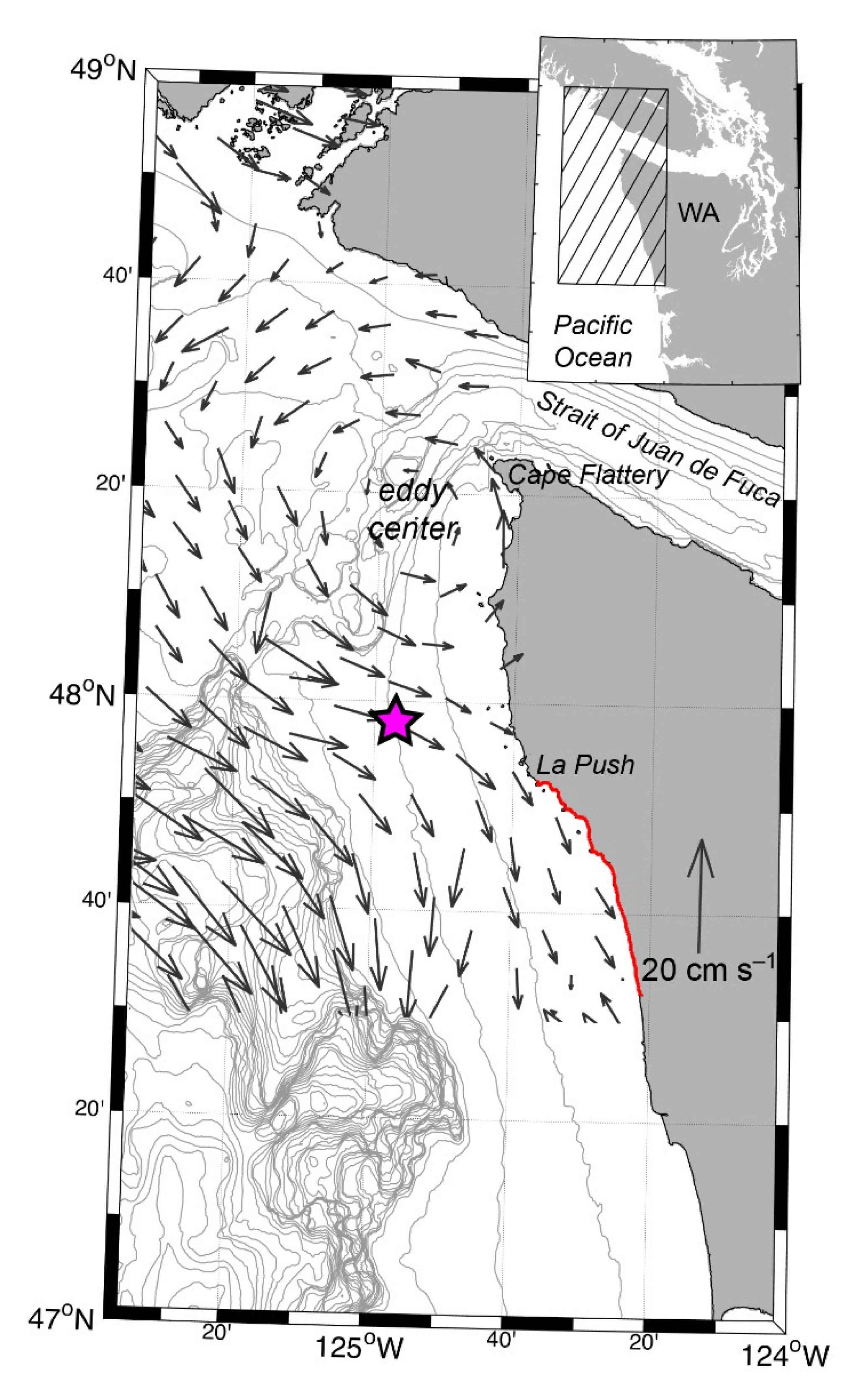
2.1. Study Region

The Pacific Northwest shelf is biologically highly productive and has a long history of HABs dating back centuries [19]. Blooms of phytoplankton, including harmful species, are fueled by nutrients delivered via inputs from the Columbia River and Salish Sea estuary, seasonal wind-driven upwelling, coastal-trapped internal waves, and interactions of tides and currents with bathymetry [20]. Blooms of Pseudo-nitzschia spp. are of particular concern along the coastal beaches [21], causing fishery closures when concentrations of DA exceed regulatory thresholds for human consumption (20 ppm, except in the viscera of Dungeness crab, for which the action level is 30 ppm [22]). Especially problematic species of Pseudo-nitzschia that have caused fishery closures in the region are P. australis and P. pseudodelicatissima [23], but local isolates of P. pungens and P. fraudulenta have been shown to produce toxin [24]. Fishery closures are effective at preventing human illness as there have been no reported cases of amnesic shellfish poisoning since DA was first detected in the region in 1991 [25]. The closures, however, cause severe economic, social, and cultural impacts to local coastal communities that rely on fisheries resources. For example, the massive 2015 HAB caused prolonged closures of the commercial Dungeness crab fishery, with the season declared a fisheries resource disaster for the Quileute Tribe on the northern Washington coast (https://media.fisheries.noaa.gov/dam-migration/69_dungeness_determination_noaa-sf.pdf, accessed on 17 March 2021), and coastal residents reported negative impacts to their sense of place, cultural identity, and emotional wellbeing [26,27]. Pacific Northwest tribal communities may be disproportionately impacted by HABs of Pseudo-nitzschia spp. due to the cultural and spiritual significance of shellfish. Shellfish feature so prominently in tribal traditions that the native language of the Quinault Indian Nation on the central Washington coast includes the phrase “ta-aWshi xa-iits’os”, meaning “clam hungry”.

Identified sources of toxic cells of Pseudo-nitzschia spp. in the Pacific Northwest are associated with two offshore retentive oceanographic features, the seasonal Juan de Fuca eddy and Heceta Bank [28,29,30,31]. The recirculating patterns of these features retain phytoplankton, including Pseudo-nitzschia spp., for longer periods of time compared to other areas of the open coastline [31,32]. Relatively low grazing rates by zooplankton compared to Pseudo-nitzschia spp. growth rates [33] and both macro- and micro-nutrient stress also likely contribute to the abundance and toxicity of Pseudo-nitzschia spp. in the eddy [28]. The Juan de Fuca eddy, located offshore of northern Washington, has been shown to be a source of toxic cells during late summer and fall [31]. Water masses carrying toxic cells can escape from the eddy and be transported southward during periods of upwelling-favorable winds. Weak storms, periods of downwelling-favorable winds, or other mechanisms leading to onshore flow can then transport the cells to coastal beaches where they can contaminate shellfish [28,31]. Heceta Bank, located off the central Oregon coast, has been shown to supply toxic cells to coastal beaches during spring when the buoyant Columbia River plume can act as a conduit [30].

The ESP mooring system described here was deployed immediately to the south/southeast of the Juan de Fuca eddy as part of the long-term Northwest Enhanced Moored Observatory (NEMO; Figure 1) that is jointly operated by the University of Washington and the Northwest Association of Networked Ocean Observing Systems (NANOOS). NEMO is located roughly 24 km west/northwest of La Push, Washington in 100 m of water and in the middle of the northwest Washington shelf. This site was selected for several reasons. First, current velocities observed at NEMO indicate that the site is located in the flow path of water escaping from the “leaky” side of the Juan de Fuca eddy during disruptive late summer/fall storms—a result that is consistent with model output [31] (Figure 1). Thus, near real-time observations enabled by the ESP may offer early warning of HABs for coastal beaches south of the NEMO site. Second, the broad range of real-time measurements already being collected and recorded at NEMO provide valuable contextual information for interpreting ESP observations. Lastly, significant cost savings and benefits arise from having access to technical expertise in combining fieldwork efforts with the existing mooring program.

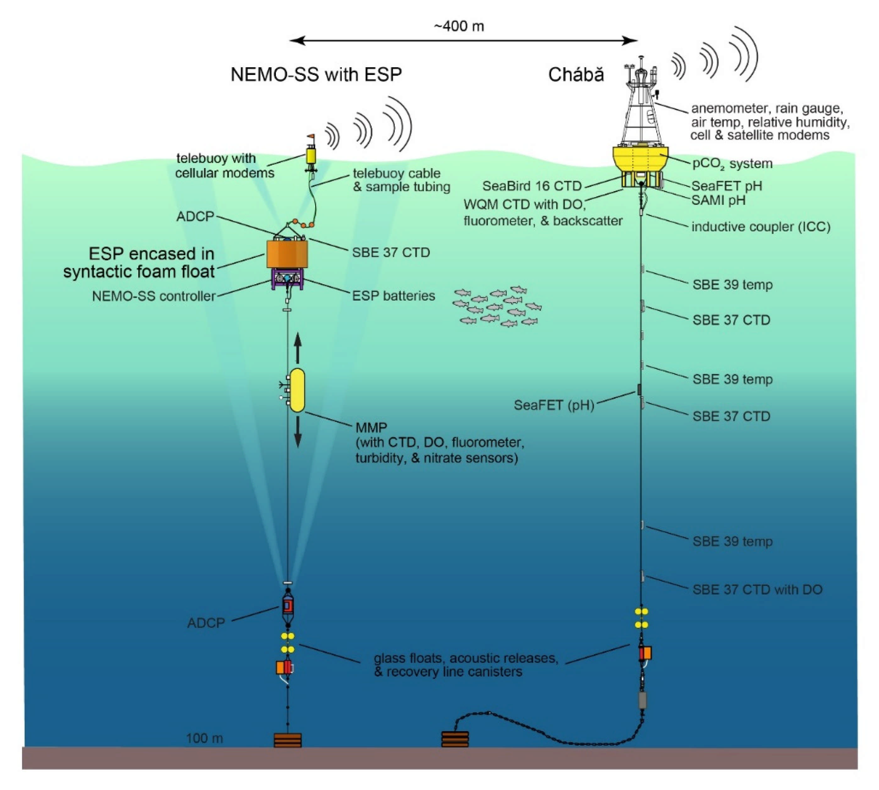
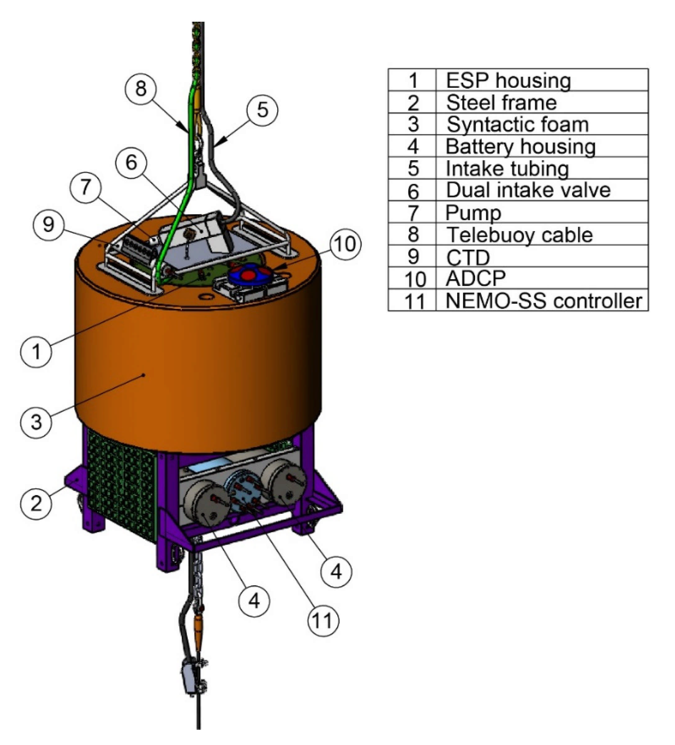
2.2. ESP Mooring Design

Established in 2010, NEMO measures surface atmospheric (e.g., surface wind, humidity, air temperature, pressure, and rainfall) and both near-surface and water-column ocean properties (pCO₂, temperature, salinity, oxygen, turbidity, nitrate, chlorophyll-a, pH, and currents; https://nwem.apl.washington.edu/about_proj_NEMO.shtml accessed on 17 March 2021). NEMO consists of a heavily instrumented surface mooring called Chábă (meaning “whale tail” in the native Quileute language) and a companion sub-surface profiling mooring ~400 m away. The ESP and its associated subsystems (power, telemetry, and pump) were integrated into the existing NEMO sub-surface profiling mooring (NEMO-SS) from 2016 through 2018. This was a relatively straightforward engineering effort that maintained the general NEMO-SS mooring configuration. Criteria and considerations when modifying the mooring design and designing/building ESP subsystems included:

• Minimizing ESP tilts and accelerations (particularly on recovery) so that they do not exceed 30 degrees from vertical and 2g (where g is the acceleration of gravity and is equal to 9.8 m/s²) to prevent damage to ESP components and spills/leaks of ESP reagents/waste;
• providing at least 5000 watt-hours of power for the ESP and its telemetry and pump systems for the ~60-day deployments;
• supporting constant, relatively high-bandwidth, two-way communications with a shore-side server;
• sampling near-surface water (1–2 m), where the highest concentrations of Pseudo-nitzschia cells were expected, without drawing air into the pumped sampling system;
• facilitating straightforward and safe deployments and recoveries;
• minimizing drag to decrease mooring knock-down in expected currents of up to 0.75 m/s;
• locating the ESP below the strong accelerations of surface wave motions, but shallower than the pressure case rating of 50-m, and ideally at pressures of ~16–18 dbars to facilitate sample collection; and
• attaining a minimum buoyancy of 226 kg to allow sufficient wire tension for a McLane Moored Profiler (MMP) to operate.

Before modification, NEMO-SS consisted of: (i) a primary-buoyancy syntactic foam float at roughly 16-m depth that held the mooring controller, (ii) a small telemetry buoy at the surface connected to the controller via a specialized telemetry cable, and (iii) a MMP recording profiles along the 75 m of mooring wire below the syntactic float. To integrate ESP and its subsystems, the foam float and its frame were replaced with a custom designed syntactic foam float, stainless steel top frame, and steel base. This infrastructure houses and supports the large ESP pressure case and two ESP battery pressure cases along with the pre-existing NEMO-SS controller pressure case, an up-looking 600 kHz acoustic Doppler current profiler (ADCP), and a Seabird 37 CTD instrument (Figure 2). To support two-way, real-time communications with ESP the telemetry cable was also modified to provide independent power and communications to a second, separate modem housed in the telebuoy. Although possible to use the ESP controller to support the pre-existing NEMO-SS sensors (MMP, ADCP, and CTD), funding limitations, power and sample rate considerations, and simplifying continuity of non-ESP deployments led to the decision to keep the two systems separate.

The galvanized and powder-coated steel base serves the dual purpose of holding the two ESP battery cases and the NEMO-SS controller case and acting as the structural “hard” point to connect the frame-float-base assembly to the mooring wire. The large (0.83 × 0.58 m, 2.2 × 10⁵ cm³), cylindrical, anodized aluminum pressure case containing the ESP sits above and is bolted to (via an adaptor plate) this steel base. The syntactic foam float, providing 544 kg of buoyancy, is a 0.8-m tall by 1.2-m diameter cylinder that also sits atop the base frame, but has a 0.7-m diameter center through-hole so that the float encircles the ESP pressure case (Figure 3). This design, with the syntactic foam surrounding the ESP, both protects the ESP from blunt-force damage while deployed and during deployment/recovery operations and also minimizes the cross-sectional area of the mooring, and thus current drag. The stainless frame and float are similar to a standard ADCP subsurface float configuration. The pyramidal stainless steel top frame has four vertical legs that pass through four holes in the foam float and bolt to the base, securing the foam in place and structurally connecting the top of the mooring to the base. This top frame provides an essential “hard” lift point for deployment operations (e.g., tagline placement) and for connecting the telebuoy cable. It additionally protects the ESP pressure case lid, equipped with bulkhead connectors and components of the pump subsystem for water sampling. To minimize galvanic corrosion, the stainless-steel frame, aluminum ESP pressure case, and steel base frame were all electrically isolated using nylon spacers with zincs added to all three isolated components. The ESP battery and NEMO-SS controller cases were made of chlorinated polyvinyl chloride (CPVC) and, thus, did not require electrical isolation. To facilitate handling and moving the frame-float-base assembly, the base frame leg height and spacing were designed to accept a pallet jack. Additionally, 5/8” pear-links were welded to each of the four base legs as tagline points for added control during overboarding. A “guard bar” that extends across the front of the ESP battery and NEMO-SS controller pressure cases was added to prevent damage, particularly from the chain connected to the base bail during deployments.

The ESP mooring design provides a substantial righting moment when the base-float-frame assembly is floating at the surface during deployment and recovery operations. This is achieved by the opposing forces of the positively buoyant ESP (150 kg buoyancy) and syntactic foam float sitting above the steel base frame containing the negatively buoyant ESP batteries and NEMO-SS pressure case. The cylindrical design of the float with the center of gravity substantially below the center of buoyancy minimizes ESP tilts with motions/accelerations largely in the vertical. This stability is enhanced by adding 9 kg lead ingots to each of the four base legs. Further, as the ESP is slowly towed behind a vessel via the mooring wire on deployment, which can impose a torque that tilts the ESP, the final design positioned the base frame’s wire/chain connection point, or bail, high and close to the center of buoyancy to minimize this twisting force.

2.2.1. ESP Power Subsystem

The ESP base frame holds two battery housings to power the instrument, each containing 200 1.5-volt alkaline D-cell batteries assembled in 10 individual battery packs configured in a 10-serial, 2-parallel (10S2P) configuration, nominally providing 15 volts. Conservatively assuming that each cell provides 11 Ah of power with a cut-off of 1.0 V, this yields approximately 5700 Watt-hours of power assuming an average operating voltage of 13 volts. Each battery pack is diode-protected to prevent current reversals and an aggregator printed circuit board mounted on the inside of the battery housing lid is equipped with a 30 Amp fuse. The two housings connect to the ESP independently via two separate Subconn bulkhead connectors on the ESP lid, ensuring continued power if one battery housing were to fail. Additionally, as each of the 20 individual battery packs per housing is diode-protected, there is a second layer of independence as individual packs can fail without influencing the performance of the others. Each battery housing is equipped with a Deep-Sea Power and Light pressure release valve to prevent the dangerous build-up of pressure from either off-gassing or heating.

2.2.2. ESP Telemetry Subsystem

The telemetry system, which supports independent cellular communications for the ESP and the NEMO-SS controller separately, consists of a small (1-m tall, 0.4-m diameter) custom-designed surface telemetry buoy (“telebuoy”) housing the two modems and signal converters, a specialized telemetry cable, and a signal converter and small signal control board within the ESP pressure case. The CPVC telebuoy pressure case is secured in the well of a cylindrical Surlyn foam float, with two cellular antennas (one for each modem) mounted on a fiberglass rod/flagpole. The design of the telebuoy, with a narrow cylindrical hull and a heavy, low, ballast ring, is intended to minimize antenna tilts that may degrade communications. Interference between the two antennas was minimal as one was operating for only ~10 min every two hours. The telebuoy cable, manufactured by Falmat, is from the Deep Ethernet series of cables and has four twisted Ethernet pairs (23 AWG) and four power conductors (20 AWG), Kevlar fibers added for a 907 kg break strength, a sparse stainless outer braid for cut protection, and both a water-block membrane and inner jacket added for increased durability. Yale grips are wrapped near each end of the 29-m long telebuoy cable to transfer the force load between the cable and the telebuoy at the top and on the steel float frame at the bottom. To lift the slightly negatively buoyant telebuoy cable away from the float frame at the bottom and prevent entanglement, eight 9” (0.2 m) diameter hard “trawl” floats mounted to 5/16” (0.9 cm) double braid line is attached in-line to the lower 6 m of the telebuoy cable.

ESP communications use the USB 1.1 protocol, but as USB is normally limited to transmission distances of <5 m, a pair of USB-Extenders (Icron Rover 1850 model) are used to extend USB to the modem using two of the telebuoy cable’s twisted pairs of CAT6 Ethernet. One extender is located within the ESP case (LEX) and the other within the telebuoy case (REX). Nominally 15 V of power is provided by two separate conductors, and is stepped down to 5 V within the telebuoy case to power to the ESP’s USB modem (Multitech Cell 100). As noted, the telemetry for NEMO-SS is largely independent of the ESP telemetry—sharing only the telebuoy cable (but not conductors) and telebuoy infrastructure. The NEMO-SS controller uses the RS-485 protocol to communicate with its modem (a Digi WAN 3G), with a RS-485 to 232 converters used within the telebuoy. At the time of ESP integration into the mooring design, RS-485 had proven to be successful over more than 5 years of NEMO-SS deployments. However, as the USB/Ethernet connection is ten times faster than RS-485 and interfaces easily with ESP, it was selected for ESP-modem communications. USB also allows adding devices to the telebuoy in future.

2.2.3. ESP Pump Subsystem

The pump subsystem consists of a sampling manifold attached to the top of the ESP frame, with a small submersible impeller pump (Aubig ZKSJ 13.2 Watt/12 V brushless) positioned downstream of this manifold to deliver near-surface (~1–2 m depth) water to the ESP situated at ~16 m depth. To potentially overcome any obstructions, the pump was selected for moderate flow rate (max 500 L/h) but substantial maximum head pressure (5 m). A 0.5” (1.27 cm) ID black Tygon supply hose, married to the telemetry cable, is connected to the upstream end of the manifold at the ESP depth and to the intake “debubbler” mounted to the telemetry cable roughly 1–2 m below the surface. Black non-toxic Tygon tubing was selected in an attempt to minimize light transmission and biofouling within the tube. The primary purposes of the debubbler are to prevent obstruction of the primary water intake and prevent air from entering the sample tubing. The final NEMO ESP debubbler design was a 0.5 m long, 2” (5 cm) OD copper pipe with an array of 0.125” (0.32 cm) diameter holes drilled near the top, oriented vertically and attached to the telemetry cable roughly 2 m below the telebuoy. The vertical orientation allowed bubbles from surface wave breaking to rise and exit the debubbler without getting pulled into the Tygon tubing, while copper was chosen for its resistance to biofouling. To further prevent obstruction of the small internal diameter tubing (0.0625”, 0.159 cm) between the manifold and ESP and internal to the ESP, #20 copper mesh with 0.034” (0.086 cm) openings is used to line the intake manifold.

2.3. ESP Configuration and Calibration

The process by which the ESP acquires and processes whole seawater samples is described in detail elsewhere [15]. In short, particulates in seawater samples (variable volume) are captured on a Durapore membrane (0.65 µm, 25-mm diam.; Millipore, USA) held inside a “collection puck” (i.e., titanium reaction chamber). Lysis/extraction is carried out inside the pressurized collection puck, with the resulting lysate/extract cleared of particles using a second Durapore membrane (0.22 µm, 25-mm diam.) held in a “lyfil puck”, and then passed to an “array” puck for analysis. For this study, ESP was configured to perform sandwich hybridization assay (SHA) to detect HAB species and competitive enzyme-linked immunosorbent assay (cELISA) to detect DA, generally following protocols described in Greenfield et al. [35,36] and Doucette et al. [37], respectively, but with several improvements (described below) to the protocol for toxin extraction and cELISA.

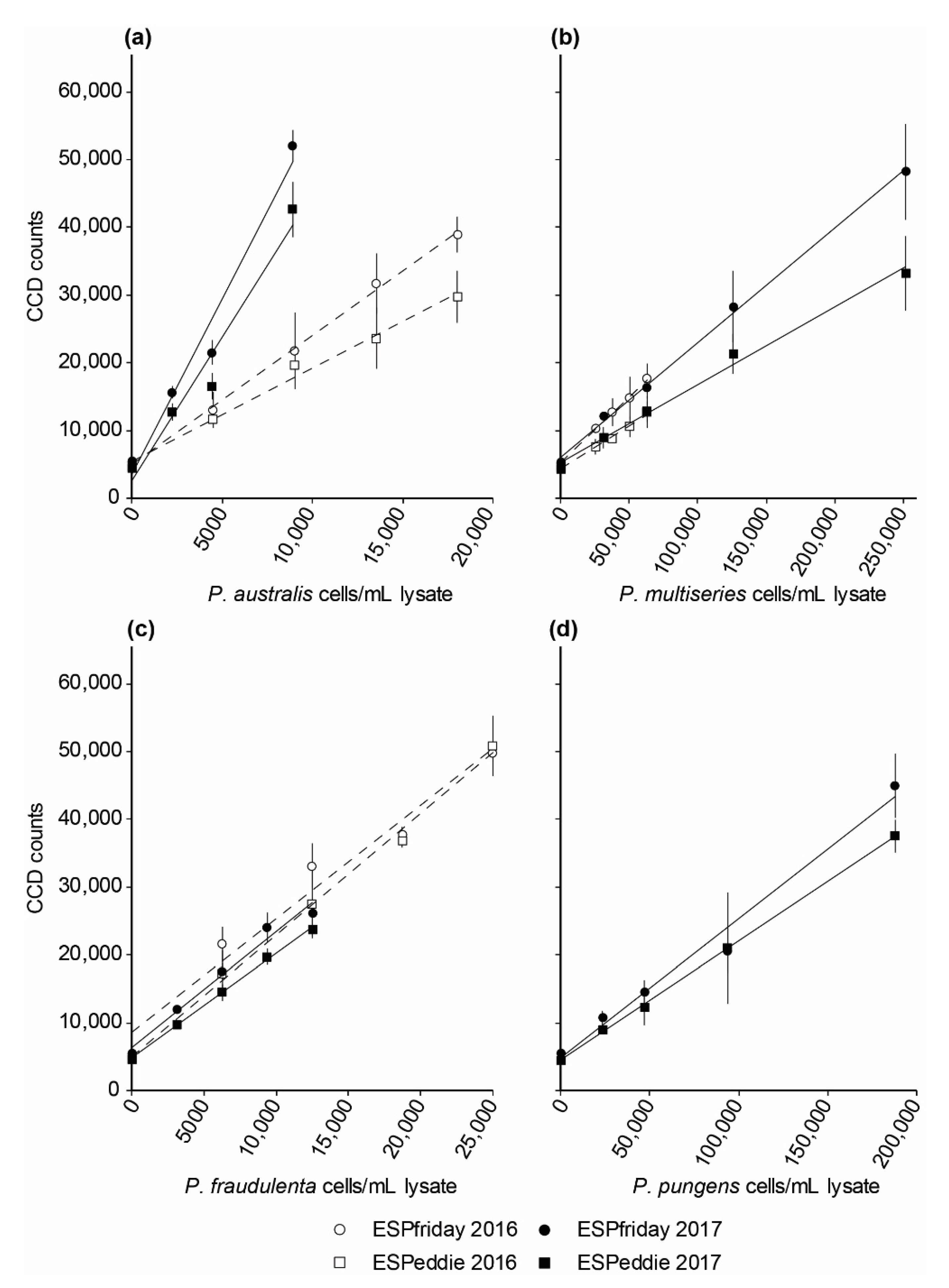
2.3.1. Harmful Algal Bloom Species Calibration

Ribosomal RNA (rRNA)-targeted DNA capture probes for P. australis (auD1), P. multiseries (muD1 and muD3), P. multiseries/P. pseudodelicatissima (muD2), P. fraudulenta (frD2), P. pungens (pung1), P. arenysensis (ary1), P. hasleana (has2), A. catenella (NA1), and H. akashiwo (Het1) were included on the HAB arrays [36,38,39,40,41]. Calibration curves were generated for the auD1, muD1, frD2, and pung1 probes only; the remaining probes on the array were monitored for activity and presence/absence of these species were reported. Prior work in the Pacific Northwest confirmed that local strains of A. catenella and H. akashiwo reacted reliably with the NA1 and Het1 probes, respectively (unpublished). Local strains of P. pseudodelicatissima, P. arenysensis, and P. hasleana were unavailable at the time of this study to confirm reactivity with the muD2, ary1, and has2 probes, respectively; however, these probes were developed using strains isolated from the same upwelling system on the U.S. West Coast (i.e., Monterey Bay, CA, USA) [38,39].

Details for the preparation of reference material, generating calibration curves for HAB targets, and for determining cell abundances are outlined elsewhere [36,39]. Briefly, U.S. West Coast isolates of target Pseudo-nitzschia species were obtained and grown in sterile, 0.2-µm filtered, natural seawater amended with f/2 nutrients and vitamins [42] at 15 °C under a 12:12 h light:dark photoperiod. Cultures were counted using light microscopy and harvested when cells were in exponential growth, with multiple aliquots low-vacuum (5 mm Hg) filtered onto individual Durapore membrane filters (0.65 µm, 25-mm diam.; Millipore, USA) and immediately stored in liquid nitrogen. Lysis employed 2.0 mL of guanidinium thiocyanate lysis buffer applied at 85 °C for 5 min, and lysates from 3 filters were filtered, combined, homogenized, and diluted as necessary before being introduced to the ESP for automated application to HAB arrays. HAB images were analyzed using ImageJ software (NIH freeware; version 1.50i) by calculating average array spot intensities using a 4 × 4 pixel block and background values were determined using a 50×50 pixel block. Background values were not subtracted from the spot intensities. Lower limits of quantification (LLOQ) for each capture probe were defined, following Greenfield et al. [36], as the value of the background plus 3 times the standard deviation of the background. Each point on the calibration curves is the average of 3 HAB arrays. Calibration curves were fit using linear regression of spot intensities (measured as counts) as a function of cells per mL lysate. Two ESPs were used in this study—ESPfriday and ESPeddie. Due to slight differences in the sensitivity between ESPs and batches of reagents, individual calibration curves for HAB targets were generated for each year and each ESP. Differences in the slopes of the relationship between spot intensity and cell concentration are small between 2016 and 2017, but there are significant differences between the two ESPs. These are shown in Figure 4 and curve parameters from linear regressions are given in

Table 1. Linear regression coefficients for the model y = α + βx (where y is spot intensity and × is cells per mL lysate; n = 3 Figure 2. values for the harmful algal bloom (HAB) species calibration curves. Coefficients are given for curves generated in 2016 and 2017 on ESPfriday and ESPeddie for P. australis auD1, P. multiseries muD1, P. fraudulenta frD2, and P. pungens pung1. The lower limit of quantification (LLOQ) refers to the lowest cell concentrations (cells/mL lysate) that could be quantified.

Year	ESP	Probe	α	β	R2	LLOQ (Cells/mL)
2016	ESPfriday	auD1	5043.6	1.8999	0.9976	434
		muD1	5362.3	0.1932	0.9986	2622
		frD2	8543.2	1.6806	0.9693	323
	ESPeddie	auD1	5386.4	1.3797	0.9888	152
		muD1	4408.0	0.1263	0.9903	9409
		frD2	5021.9	1.7922	0.9953	627
2017	ESPfriday	auD1	3440.0	5.1888	0.9706	484
		muD1	6090.2	0.1693	0.9979	4099
		frD2	6380.1	1.7112	0.9784	405
		pung1	4843.9	0.2051	0.9828	5396
	ESPeddie	auD1	2555.6	4.2469	0.9587	697
		muD1	5347.1	0.1144	0.9911	1471
		frD2	4812.5	1.5423	0.9980	456
		pung1	4466.7	0.1758	0.9996	5964

. Note that calibration curves were developed for HAB targets in 2016 and 2017 only; presence/absence of HAB targets was reported in 2018.

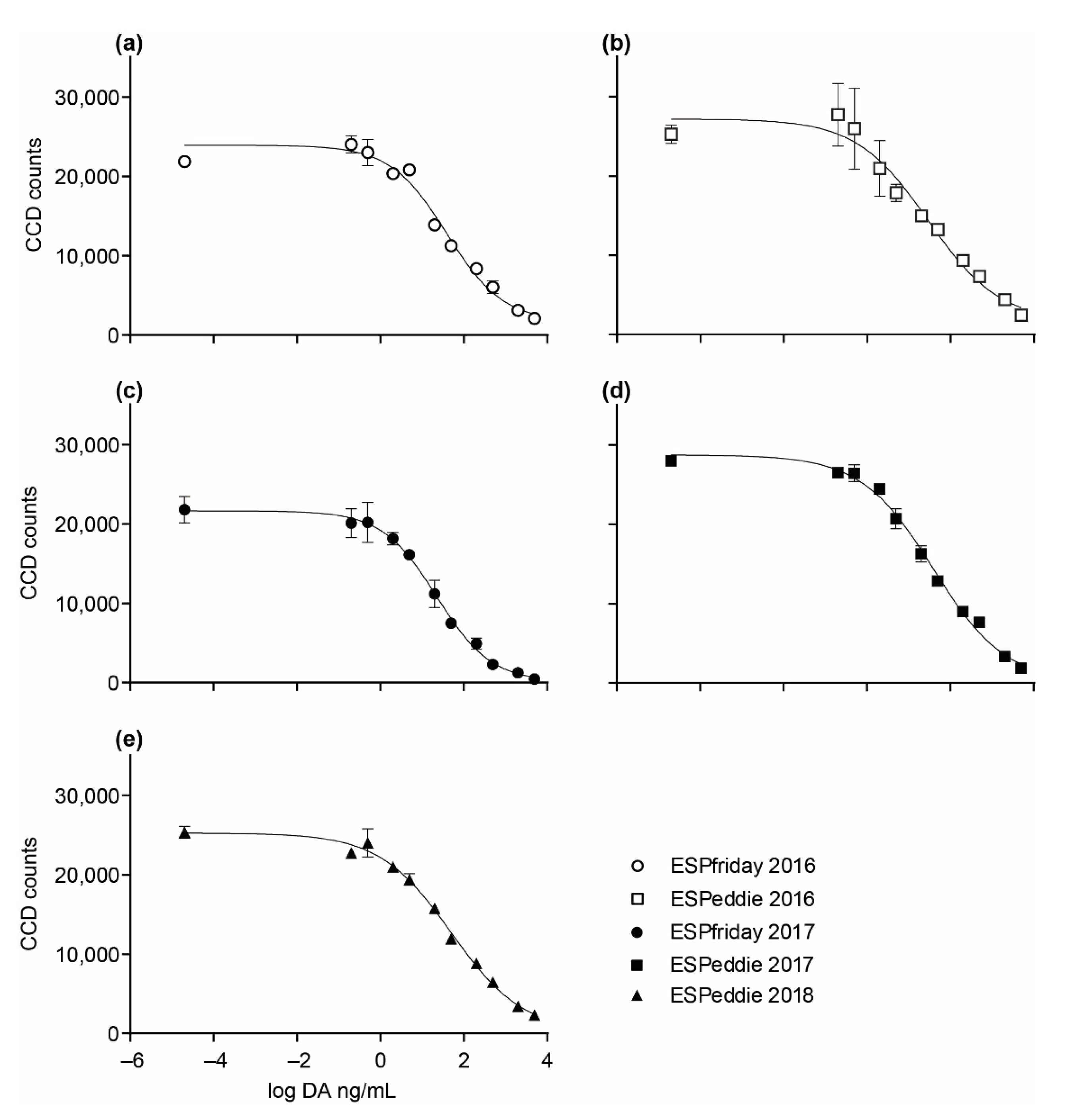
2.3.2. Domoic Acid Calibration

Toxin extraction onboard ESP employs 2.0 mL of 50% aqMeOH containing 0.01% Tween-20 (Sigma, St. Louis, MO, USA) applied at 70 °C for 10 min. The cELISA incorporates an anti-DA polyclonal primary antibody (Queen’s University Belfast) and a membrane-based array (Optitran BA-S 83 reinforced nitrocellulose; Whatman, MA, USA), on which are printed 21 features comprising DA-ovalbumin conjugate (14 features; 0.14 mg/mL DA-ovalbumin, 2.9X SSPE (Sigma, USA) in water) and rabbit IgG (7 features; 0.0075 mg/mL rabbit IgG, 1.0 mg/mL NeutrAvidin (ThermoFisher Scientific, Waltham, MA, USA), 2.9X SSPE, 5 nM betamercaptoethanol in 3% aqMeOH) (additional details in [37]). The DA-ovalbumin conjugate was used to quantify toxin levels, whereas the rabbit IgG served as an internal control, confirming assay chemistry integrity, and to meter autoexposure of array images captured by the onboard CCD camera. The array was blocked (Western Blocker™, Sigma, USA), exposed to toxin extract (or certified reference calibration standard) combined 1:1 with primary antibody (1:3000 in S/D/B buffer (ThermoFisher Scientific, USA); 28 ± 2 °C; 8 min), washed with blocking reagent, treated with goat anti-rabbit secondary antibody-HRP conjugate (1:9500 in S/D/B buffer (ThermoFisher Scientific, USA); 28 ± 2 °C; 8 min), washed, and features visualized using a chemiluminescent substrate reporter (SuperSignal™ West Femto Maximum Sensitivity Substrate, ThermoFisher Scientific, USA) prior to imaging. The mean pixel intensity of individual features was quantified using ImageJ software (NIH freeware; version 1.52e) and employed to generate calibration curves and quantify particulate toxin levels (details below). Arrays were considered acceptable when the percent coefficient of variation (% CV) for the mean pixel intensity of all features within the toxin or control groups were 20% or less.

Calibration curves were generated within about a month prior to each deployment using DA certified reference material (CRMP, NRC Canada) to formulate 10 toxin standard concentrations ranging from 0.2 to 5000 ng/mL (0.2, 0.5, 2.0, 5.0, 20, 50, 200, 500, 2000, 5000 ng/mL) as well as a 0 ng/mL negative (n = 2 for all values) diluted in non-toxic Pseudo-nitzschia cell matrix equivalent to 1,000,000 cells/L in 50% aqMeOH + 0.01% Tween-20. Response data were fitted to a 4-parameter logistic function (variable slope), described by the Hill slope (steepness of curve) and a “goodness of fit” R² statistic (Figure 5;

Table 2. Parameters for the domoic acid (DA) calibration curves on ESPfriday and ESPeddie in 2016, 2017, and 2018. Parameters are determined based on a 4-parameter logistic fit (variable slope) of signals generated by DA certified reference material tested at 10 concentrations ranging from 0.2 to 5000 ng/mL, as well as a 0 ng/mL negative (n = 2 for all values). The EC₅₀ represents the half-maximal response, whereas the EC₈₀ and EC₂₀ represent the lower and upper limits or boundaries, respectively, of the linear dynamic range within which responses can be quantified accurately (i.e., LLOQ and ULOQ). The lower limit of detection (LLOD) refers to the lowest toxin concentration (ng/mL) that can be detected but not quantified reliably (see text for additional details).

Year	ESP	Slope	R2	EC50	EC80	EC20	LLOD (ng/mL)
2016	ESPfriday	−0.642	0.978	38.93	4.48	338.03	1.81
	ESPeddie	−0.504	0.942	29.02	1.85	455.21	1.48
2017	ESPfriday	−0.663	0.955	22.42	2.77	181.66	1.95
	ESPeddie	−0.501	0.989	38.97	2.45	619.70	1.32
2018	ESPeddie	−0.502	0.988	50.23	3.17	794.85	1.40

). The EC₅₀ represents the half-maximal response, and the EC₈₀ and EC₂₀ describe the lower (i.e., LLOQ) and upper (i.e., upper limit of quantification; ULOQ) boundaries of the linear dynamic range, respectively, over which responses can be quantified accurately. Responses for sample unknowns generated during deployments were quantified via interpolation. The assay lower limit of detection (LLOD) was calculated by adding two standard errors of the intensity at the top of the curve to the LLOQ (EC₈₀) and converting to the antilog. All of the preceding calculations were performed using “in assay” values. The numbers reported as the LLOD, LLOQ, and ULOQ were calculated from values generated from the calibration curve and converted to ng/L of ambient water, based on the volume filtered for each sample.

2.4. ESP Deployments

The ESP mooring was deployed in the spring and fall of 2016 and 2017, and in the fall of 2018. For the 2016 and 2017 deployments, ESP was programmed to run the “HABDA” protocol immediately upon deployment and then three times per week at 1400 PDT on Sunday, Tuesday, and Thursday. The HABDA protocol commands ESP to filter a seawater sample and perform SHA for HAB targets (~3 h), and then filter a second seawater sample and perform cELISA for particulate DA (~2 h). The sample volume for HAB and DA samples was set to 1 L; however, ESP automatically reduces the sample volume to avoid bursting cells if the pressure required to filter the sample at 0.2 mL/s exceeds 13 PSI. For the 2018 deployment, ESP was programmed to run the HABDA protocol upon deployment and then once per week at 1400 PDT on Sunday, and the DA protocol four times per week at 1700 PDT on Monday, Tuesday, Wednesday, and Thursday. Additional DA protocols were programmed at 0500 PDT during the second week of the 2018 deployment to examine the potential effects of diurnal convective overturning on patterns in DA concentrations. Active deployment periods (i.e., when the ESP was operational) and a summary of target analytes for each deployment are given in

Table 3. Dates when ESP was actively sampling (i.e., active deployment period), target analytes, and the total number of samples analyzed for each deployment on the Washington shelf. “Q” indicates that the target analyte was quantitatively determined and “+/−” indicates that it was monitored for presence/absence only. Target analytes are Pseudo-nitzschia australis (auD1), P. multiseries (muD1), P. fraudulenta (frD2), P. pungens (pung1), Alexandrium catenella (NA1), Heterosigma akashiwo (Het1), and particulate domoic acid (pDA).

Year	Season	ESP	Active Deployment Period	Target Analyte							Total # Samples
				auD1	muD1	frD2	pung1	NA−1	Het1	pDA
2016	Spring	ESPfriday	23 May–10 July	Q	Q	Q	+/−	+/−	+/−	Q	42
	Fall	ESPeddie	9 September–18 October	Q	Q	Q	+/−	+/−	+/−	Q	34
2017	Spring	ESPfriday	2 May–27 June	Q	Q	Q	Q	+/−	+/−	Q	42
	Fall	ESPeddie	6 September–15 October	Q	Q	Q	Q	+/−	+/−	Q	34
2018	Fall	ESPeddie	6–20 6 September	+/−	+/−	+/−	+/−	+/−	+/−	Q	17

.

The deployment of the ESP is a modification of a typical anchor-last subsurface mooring deployment to minimize accelerations and tilts on the instrument. With the mooring largely assembled and the 75 m Nilspin mooring wire wound on a deck winch, the telebuoy and telebuoy cable are hand-deployed and streamed astern of the vessel. Next, the syntactic foam float/base frame and the ESP are deployed over the stern using an A-frame or crane and a mechanical release. The vessel continues to slowly move ahead with the telebuoy and ESP/float/frame, presently at the surface, streaming out behind the vessel. Then, the McLane profiler, ADCP, and acoustic releases are all connected sequentially in-line along the mooring and deployed over the stern using the winch and A-frame. Lastly, the 1100-kg air-weight steel anchor, which is positioned at the stern, is connected to complete the mooring. However, instead of mechanically releasing the anchor from the surface to deploy the mooring, we use a working line on the winch to lower the anchor to within about ~20 m of the bottom (80-m depth) prior to releasing it acoustically. With the vessel continuing to move ahead at ~1 kt through the water, the anchor is slowly lowered, bringing the ESP/float/frame close to the stern of the vessel due to the changing geometry of the mooring wire. Just prior to the ESP submerging, while it is within a few meters of the vessel’s stern, the anchor is acoustically released from the working line. This deep anchor release significantly reduces tilts and accelerations on the ESP that would occur if the anchor were released from the surface.

3. Results

The five deployments of the ESP mooring system over three years of field operations from 2016–2018 were successful in achieving the mission of providing critical data on the concentrations of HAB species and particulate DA. In total, the ESP acquired and analyzed 79 seawater samples using SHA for HAB species and 90 seawater samples using cELISA for particulate DA. The target volume of 1L was filtered by the ESP for 89% of the samples, with smaller volumes (375–950 mL) analyzed for the remaining samples due to clogging of the collection filter. Figure 6 shows the concentrations of Pseudo-nitzschia species targeted for quantification (P. australis, P. multiseries, P. fraudulenta, and P. pungens; Figure 6a–d), reactivity of all SHA probes on the HAB arrays (auD1, frD2, muD1, pung1, ary1, has2, muD2, muD3, NA1, and Het1; Figure 6e–i), and the concentration of particulate DA in seawater as well as DA in razor clams collected from ocean beaches in Jefferson County, WA (Figure 6j–n; see Figure 1 for location of Jefferson County beaches). Razor clam samples were collected and analyzed by the Washington State Department of Health as part of their regular shellfish biotoxin monitoring program. Note that the “total” concentrations of Pseudo-nitzschia species targeted for quantification (hereafter total Pn quantified) is likely an underestimate of the actual total Pseudo-nitzschia species abundance, as P. pungens was not quantified in 2016 and P. arenysensis, P. hasleana, and P. pseudodelicatissima were monitored for presence/absence only. Additionally, other Pseudo-nitzschia species for which ESP does not have a probe may have been present, and therefore not detected. Nevertheless, the species of potentially toxic Pseudo-nitzschia monitored by ESP include those that are thought to most commonly cause shellfish closures in the region [23].

Section 3.1 describes the patterns observed across all three years of ESP operations. During the 2016 and 2018 deployments, the concentration of total Pn was generally low and particulate DA was observed only occasionally, whereas higher and more consistent detections occurred during the 2017 deployments, particularly in the fall of 2017. Domoic acid was detectable in razor clams during all three years of ESP field operations but did not exceed the regulatory action level of 20 ppm. Section 3.2 and Section 3.3 interpret the patterns in total Pn quantified and particulate DA concentrations observed in 2017 in relation to the physical and chemical oceanography using data provided by collocated sensors on the NEMO platform.

3.1. Overview of ESP Observations and Mooring Performance

In spring 2016, concentrations of Pseudo-nitzschia species targeted for quantification by ESP were below the LLOQ with the exception of some low-level (<1.0 × 10⁴ cells/L) detections of P. fraudulenta on 23, 26, and 29 May, 9 and 28 June, and 3 July (Figure 6a). Other detections of species monitored for presence/absence included P. arenysensis on 16 and 21 June, A. catenella on 26 and 31 May, and H. akashiwo on 19 June (Figure 6e). Five of 21 samples contained particulate DA concentrations greater than the LLOQ, ranging from 6.3–10.4 ng/L. The day prior to the ESP deployment (22 May), no DA was detected in razor clams from Jefferson County. In the next razor clam sample collected from Jefferson County beaches (21 June), the DA level was 5 ppm but decreased to 1 ppm on 5 July (Figure 6j). This was the first deployment of the ESP mooring system in a coastal shelf environment and it performed well, but spotty communications from 27 June through 12 July occasionally impacted near real-time data transmission.

In fall 2016, the total Pn quantified reached 7.8 × 10⁴ cells/L on 22 September and 2.7 × 10⁴ cells/L on 29 September and was dominated by P. multiseries (i.e., 88% and 89%, respectively), with P. australis and P. fraudulenta comprising the remainder in approximately equal amounts (Figure 6b). Pseudo-nitzschia pungens, which was not quantified in 2016, had the most detections of any species during the deployment—9 out of 10 samples from 9 September through 2 October. Other detections of species monitored for presence/absence included P. hasleana on 20 and 22 September and P. arenysensis on 29 September (Figure 6f). Detection on the muD2 probe on 22 September was likely P. multiseries (and not P. pseudodelicatissima) given the positive reactivity on the muD1 and muD3 probes on the array. The concentration of particulate DA was 46.6 ng/L at the start of the deployment on 9 September, dropped to below the LLOQ on 11 September, and then steadily increased to 138.4 ng/L on 18 September (Figure 6k). By 25 September, particulate DA had decreased to less than the LLOQ and remained undetectable. Domoic acid was not detected in razor clams from Jefferson County immediately prior to the deployment (30 August) and was between 4–7 ppm during the deployment. Operations were (remotely) temporarily suspended on 14 October ahead of a large storm that moved through the region to reduce the risk of instrument malfunction. Communications with ESP were lost during the storm, but reestablished on 18 October enabling the mission to be resumed. On 19 October, however, the ESP’s computer crashed due to memory shortage stemming from a large number of error messages being generated when communications could not be established during the storm. This software glitch (which was corrected for future deployments) prevented the final four samples of the mission from being collected and analyzed.

In spring 2017, the total Pn quantified reached 8.1 × 10⁴ cells/L early in the deployment on 9 May and was largely comprised of P. pungens (55–90%) (Figure 6c). Pseudo-nitzschia australis and P. fraudulenta were also observed during this time, comprising 3–11% of the total Pn quantified. Pseudo-nitzschia multiseries was detected on 9 May at 3.0 × 10⁴ cells/L (i.e., 37% of total Pn), but this detection is questionable as positive reactivity was recorded on the muD1 probe only and not the more sensitive muD2 and muD3 probes [36,39]. Relatively low abundances of P. australis and P. fraudulenta were detected on 14 May (1.3 × 10⁴ cells/L) and 1 June (0.2 × 10⁴ cells/L), but total Pn quantified otherwise remained below the LLOQ. Other detections of species monitored for presence/absence included P. arenysensis on 2 and 9 May and P. hasleana on 1, 4, and 15 June. Positive reactivity on the muD2 probe on 14 May likely indicated the presence of P. pseudodelicatissima (and not P. multiseries) as no activity was detected on the muD3 probe (which has comparable sensitivity to P. multiseries as the muD2 probe on ESP [39]). Alexandrium catenella was detected in five of 10 samples from 2 May to 1 June and was absent from the remaining samples, while H. akashiwo was not detected in any samples (Figure 6g). At the beginning of the deployment on 2 May, the particulate DA concentration was 37.0 ng/L (Figure 6l) and increased to 274 ng/L on 9 May before it decreased to below the LLOD on 28 May. The concentration of domoic acid in razor clams from Jefferson County was 18 ppm on 3 May and declined to 3 ppm on 25 June (Figure 6l). The ESP mooring system performed well during this deployment, with the exception of a flow meter (part of the pump subsystem) that failed on 16 May. Environmental Sample Processor operations were (remotely) temporarily suspended until a technician could visit the mooring site and verify that the pump itself was still operational. Operations were resumed on 28 May.

In fall 2017, the total Pn quantified was below the LLOQ at the start of the deployment on 6 September, increased to 4.6 × 10⁴ cells/L on 12 September, dropped to below the LLOQ on 14 September, and then dramatically increased to 2.3 × 10⁵ cells/L on 17 September, the highest total observed during any of the deployments (Figure 6d). For the remainder of the deployment, the total Pn quantified fluctuated between 5.0–16 × 10⁴ cells/L except for 19 September and 3, 5, and 17 October when it was below the LLOQ. Pseudo-nitzschia pungens largely dominated the total Pn quantified (86–100%) with P. fraudulenta making up the rest (5–14%), except on 17 September and 1 October when P. multiseries comprised 54% and 40% of the total Pn quantified, respectively. Note, however, that positive reactivity was not recorded on the muD2 and muD3 probes on 17 September, nor on the muD3 probe on 1 October. Pseudo-nitzschia australis was detected only once, on 8 October, and comprised only 2% of the total Pn quantified in that sample. Other detections of species monitored for presence/absence included P. hasleana, which was present in almost half of all samples analyzed, and likely P. pseudodelicatissima on 10 and 12 September and 8 October based on positive reactivity on the muD2 probe but not the muD1 and muD3 probes (Figure 6h). Alexandrium catenella was detected in five of 17 samples and H. akashiwo was detected in six of the first nine samples and was then absent from the remaining samples (Figure 6h). Concentrations of particulate DA were above the LLOD in 15 of 17 samples, and quantifiable in 13 of 17 samples (Figure 6m). During the first two weeks of the deployment, particulate DA fluctuated between the LLOD and 40 ng/L. On 21 September, particulate DA increased to 74 ng/L and on 5 October it jumped to 427 ng/L—the highest concentration observed during any of the deployments. It then fluctuated between 11 and 281 ng/L for the remainder of the deployment. Concentrations of DA in razor clams from Jefferson County remained low throughout the deployment, starting out at 1 ppm on 6 September and reaching a maximum of 6 ppm on 5 October (Figure 6m). While the ESP mission (i.e., sample collection and analysis) proceeded without interruptions during this deployment, communications became spotty on 13 September and impacted near real-time data transmission. Communications were lost on 19 September and remained mostly down for the remainder of the deployment, with only a few connections lasting long enough to transfer meaningful data to the shore station. One of those connections was 6 October and alerted managers to the significant spike in particulate DA measured on 5 October, immediately prior to a weekend opening of the recreational razor clam fishery.

In fall 2018, HAB species were monitored for presence/absence only and less frequently compared to the 2016 and 2017 deployments, whereas particulate DA was monitored at higher frequency. No Pseudo-nitzschia species were detected in the three SHA samples collected. The only other detection was A. catenella on 16 September (Figure 6i). At the beginning of the deployment on 6 September, the particulate DA concentration was below the LLOD and then increased to 27.1 ng/L on 11 September before it decreased to below the LLOD on 13 September and remained undetectable (Figure 6n). Concentrations of DA in razor clams from Jefferson County were low during the deployment, reaching a maximum of 2 ppm on 12 September (Figure 6n). The communications subsystem of the ESP mooring performed poorly during this deployment. The ESP was unable to sustain cellular communications to the shore station, resulting in repeated attempts to reestablish a connection that exhausted the onboard battery power and prematurely ended the mission almost 3 weeks before the scheduled end date.

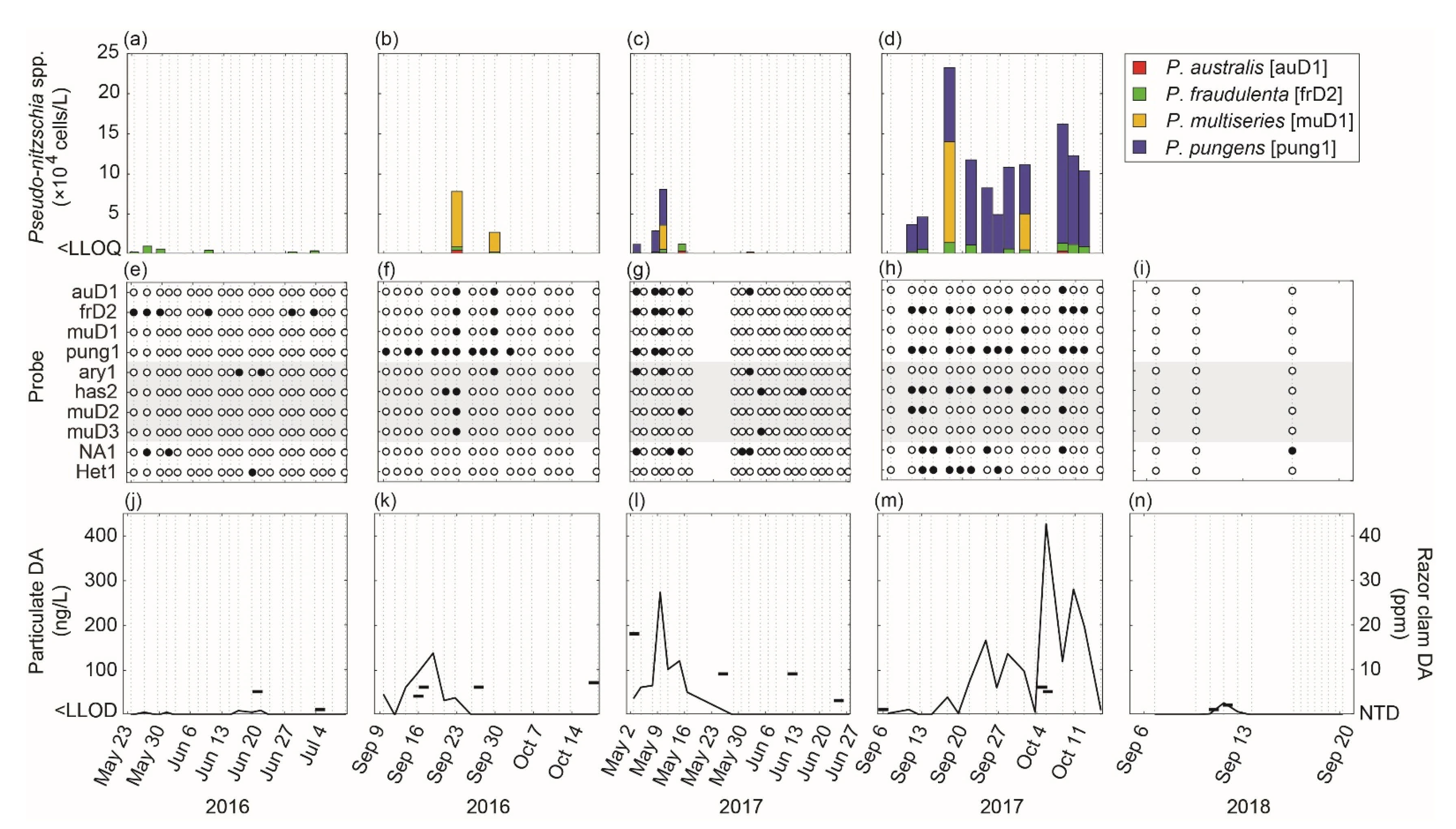
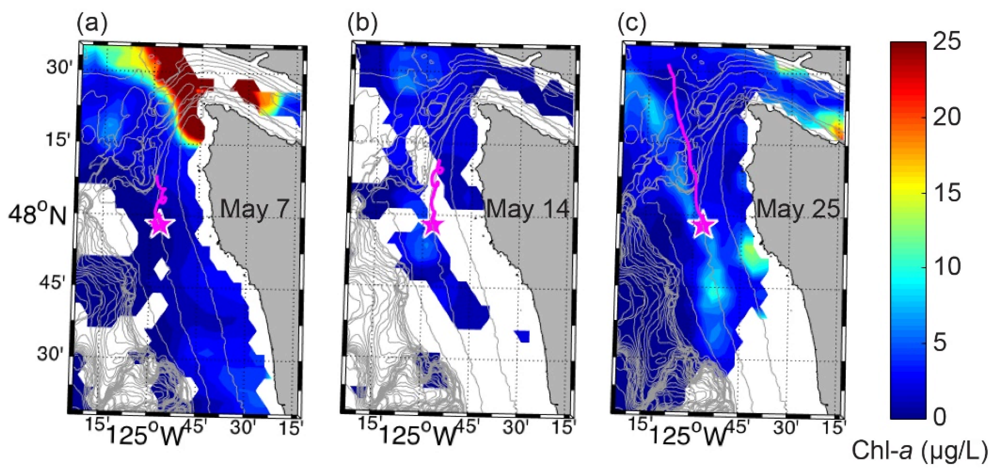
3.2. Spring 2017 Synthesis

The full value of this mooring system is realized when the above ESP observations are merged with the comprehensive suite of contextual measurements. Figure 7 shows the time series of selected physico-chemical variables measured in situ by the NEMO-SS and ChăBá moorings alongside of the total Pn quantified and particulate DA concentrations from 1 May until 1 June 2017. The early May period captured the transition to upwelling favorable local winds, which occurred 53 days later than normal in 2017 according to the spring transition index at 48° N (https://oceanview.pfeg.noaa.gov/erddap/tabledap/cciea_OC_STI.html?time,sti&latitude=48, accessed on 19 October 2020). Note that the spring 2017 deployment extended through June 27; however, ESP observations of Pseudo-nitzschia spp. and particulate DA were undetectable beyond 1 June and so these data are not shown in Figure 7. Total Pn quantified and particulate DA concentrations are overplotted on the continuous time series of chlorophyll-a in Figure 7b to examine their variations in the context of the larger phytoplankton community. To provide spatial context to the mooring observations, maps of chlorophyll-a derived from the Visible Infrared Imaging Radiometer Suite (VIIRS) onboard the Suomi-NPP satellite were examined where the NEMO-SS and ChăBá moorings were deployed for days without cloud cover. VIIRS data were obtained from NASA’s OceanColor Web (https://oceancolor.gsfc.nasa.gov/, accessed on 20 June 2020). Surface chlorophyll is generated using the blue-green reflectance ratio empirical approach of O’Reilly et al. [43], adjusting the algorithm for the VIIRS spectral bands. Specifically, the algorithm is a 3-band algorithm (OC3V, Ocean Chlorophyll 3-band algorithm for VIIRS) whose inputs are the water-leaving radiance at wavelengths of 443, 486, and 551 nm. The spatial resolution for the level 3 gridded product is 4.6 km in latitude and 3.1 km in longitude at the mooring site. The VIIRS near-surface chlorophyll-a concentrations for the grid box that contains NEMO are overplotted in Figure 7b, and show general agreement between in situ observations at 1 m depth and daytime satellite-derived chlorophyll-a.

Total Pn quantified (and particulate DA) began to increase around 7 May, about 2 days before chlorophyll-a began to appreciably increase (Figure 7b). These responses may have been a consequence of the steady shoaling of deeper water with higher nutrient concentrations over the first 10 days of the month (Figure 7e), potentially aided by a ~5 day stretch of (northerly) upwelling favorable winds (Figure 7a). Surface currents were strong and to the south at ~0.4 m s⁻¹ suggesting that this water was advected from the north. A VIIRS image from 7 May showed high concentrations of chlorophyll-a at the western entrance of the Strait of Juan de Fuca that were unrelated to the Juan de Fuca eddy (Figure 8a). Although ADCP-estimated flow paths suggest this water may have been advected into the region (Figure 8a), observations at NEMO suggest local shoaling of high-nutrient water could have been responsible for local bloom formation. These observations showed that when northerly winds slackened and then reversed around 10 May, isotherms, isohalines, dissolved oxygen contours, and nutrient contours all initially relaxed (or deepened). However, with the onset of a stronger southerly wind burst on 12 May, which was accompanied by the reversal of deep along-shelf currents, all iso-lines rapidly shoaled or rebounded and stratification in the 20–50 m depth range greatly increased (Figure 7a,c,e,f). This brought nutrients up into the euphotic zone and chlorophyll-a continued to increase whereas total Pn quantified and particulate DA decreased. Chlorophyll-a remained elevated until May 17 and then rapidly dropped, coincident with a rapid drop in nitrate levels. Although a VIIRS image from 14 May did not include measurements at NEMO due to cloud cover, steady flow from the north coupled with low (<5 µg L⁻¹) concentrations of chlorophyll-a in potential source water regions to the north (Figure 8b) suggest that the bloom observed at NEMO was largely a local response. The rapid vertical movement of all iso-lines in the 20–50 m depth range from 12 to 16 May were associated with along-shelf flows at depth, such that peaks in northerly flow were coincident with local peaks in iso-lines. This suggests a northward-propagating internal wave event. The period of this event, which is on the order of a week, as well as some correlation to wind changes, suggests this was specifically a coastal-trapped internal wave. These wind-driven, northward-propagating waves are ubiquitous on the shelf of California Current System [44,45] and have been detected at this site [46]. It is worth noting that this lower-frequency oscillation was superimposed on a strong internal tide field with a semidiurnal period (12.4 h) [46] (Figure 7f). The shallow response showed warming, freshening, and increased dissolved oxygen concentrations in the 15–25 m depth range during this time, consistent with downwelling and/or increased wind-driven mixing (Figure 7c,d). This response, however, was opposed by the lifting of iso-lines, presumably by the internal wave event, to result in very strong vertical gradients from 20–50 m depth.

A second stretch of upwelling favorable winds began around 19 May. With the onset of upwelling, nutrient contours steadily shoaled and chlorophyll-a increased. Alongshore surface currents were strong and to the south. A VIIRS image from 25 May showed some patches of high chlorophyll-a close the coast with a band of elevated chlorophyll-a along the shelf (Figure 8c). Unfortunately, ESP operations were temporarily suspended during this time due to the failed flow meter on the pump subsystem (see Section 3.1) and so we are unable to determine if Pseudo-nitzschia spp. and particulate DA also responded to this period of upwelling favorable conditions. Chlorophyll-a decreased when northerly winds relaxed around 30 May, and ESP observations of total Pn quantified and particulate DA remained undetectable for the remainder of the deployment.

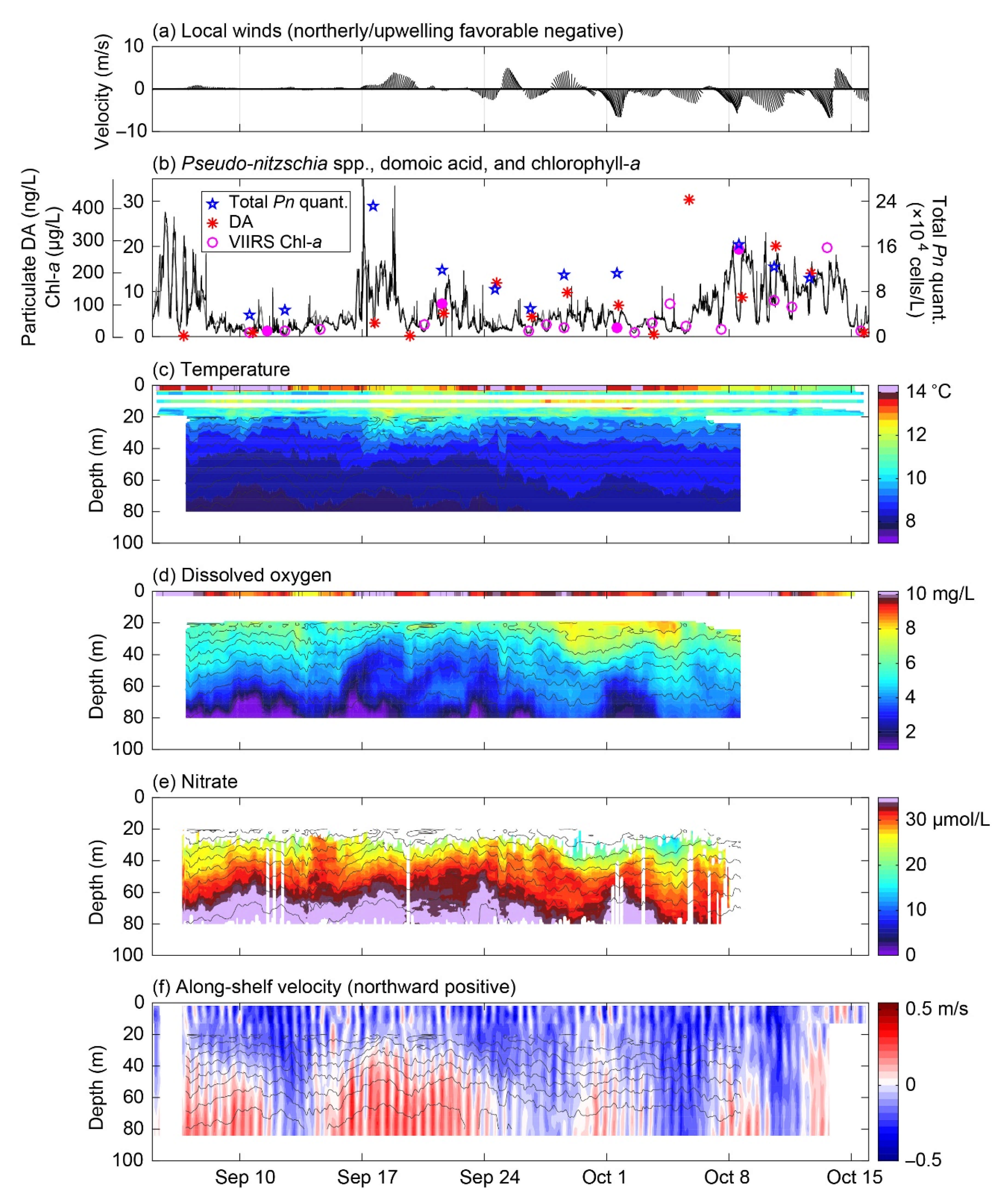
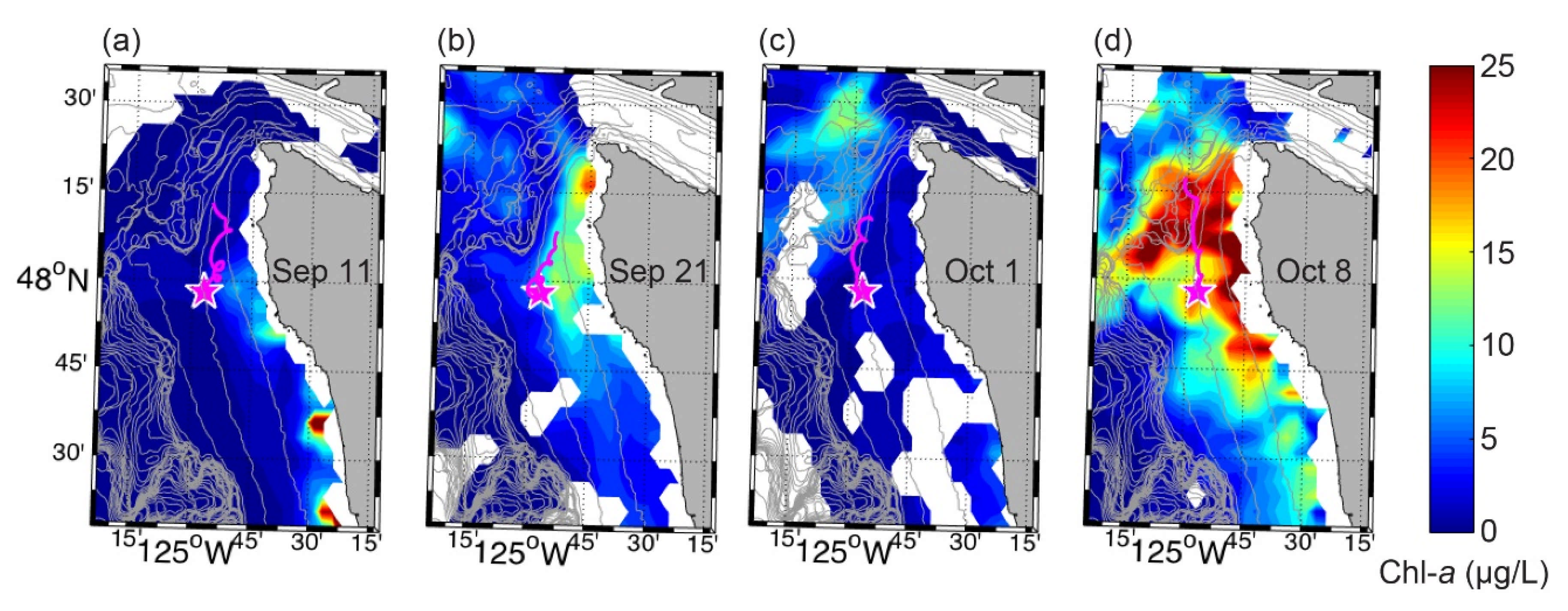
3.3. Fall 2017 Synthesis

Compared to the spring 2017 deployment period, winds were weaker and more variable, surface water temperatures were 1–2 °C warmer, and measured nutrient levels (i.e., 20–80 m depth range) were much higher during the fall 2017 deployment (Figure 9). Along-shelf velocities showed predominantly southward shallow flow during the deployment, but with frequent flow reversals below ~25-m depth. Again, the frequency of these reversals and relationship to vertical displacements of water property iso-lines suggests they are northward-propagating coastal-trapped internal waves superimposed on a strong semi-diurnal internal tide. As in the spring, northward deep flow events were generally associated with colder temperatures, higher salinities, lower dissolved oxygen concentrations, and higher nutrients at depth.

Winds were very weak during the first ~10 days of the deployment, allowing heat to build up in the surface waters from solar warming (Figure 9a,c). During this time chlorophyll-a, total Pn quantified, and particulate DA were relatively low (Figure 9b). A VIIRS image from 11 September showed low (<5 µg/L) concentrations of chlorophyll-a along most of the shelf, particularly to the north of the NEMO site and including the Juan de Fuca eddy region, a possible source of the shallow (<15 m) water reaching the NEMO site (Figure 10a). This prolonged period of very weak winds ended on 17 September when a 3-day stretch of downwelling favorable winds began, mixing the surface waters to ~30-m depth (Figure 9c). On September 16, before the winds shifted, chlorophyll-a began to increase (Figure 9a,b), potentially in response to shoaling nutrient contours and flow reversals at depth associated with an internal wave (Figure 9e,f). The chlorophyll-a response, however, may also have been enhanced by further wind-driven vertical mixing of nutrients into the euphotic zone. Total Pn quantified increased along with chlorophyll-a, but particulate DA did not exhibit as large a response, increasing only slightly from <LLOD to 40 ng/L (Figure 9b). Chlorophyll-a and total Pn quantified decreased on 19 September but then slightly increased again on 21 September, coincident with a second pulse of deep, northward along-shelf flow and shoaling of nutrient contours (Figure 9e,f). Particulate DA also slightly increased at this time to 74 ng/L (Figure 9b). A VIIRS image from 21 September showed elevated chlorophyll-a on much of the northern Washington coast shelf, with the highest values immediately south of Cape Flattery (Figure 10b). As winds were weak during this period, this pattern may be a consequence of inshore upwelling from remotely forced coastal-trapped waves [44], the presence of which is suggested by the deep current reversals and related vertical displacements (Figure 9f). Chlorophyll-a, total Pn quantified, and particulate DA remained somewhat elevated through 5 October. Winds were variable during this time, oscillating between upwelling and downwelling favorable conditions (Figure 9a), which has been shown to produce a more retentive Juan de Fuca eddy [34]. Indeed, a VIIRS image from 1 October showed elevated chlorophyll-a (~10 µg/L) in the vicinity of the eddy (Figure 10c). On 5 October, particulate DA spiked to the maximum value observed (427 ng/L); however, chlorophyll-a was low and no Pseudo-nitzschia spp. were detected (DA can sometimes be detected by the ESP in the absence of any quantifiable detections of Pseudo-nitzschia spp. because (1) the analyses for species abundance and toxin concentration are performed on separate water samples taken sequentially, (2) the assay for domoic acid is more sensitive than the SHA for some Pseudo-nitzschia spp., and (3) the presence of toxin-producing species of Pseudo-nitzschia that the ESP does not detect) (Figure 9b and Figure 6h). Additionally, nitrate levels were the lowest measured during the deployment (Figure 9e). Chlorophyll-a increased on 7 October and remained elevated until 14 October, coincident with a week-long stretch of relatively strong upwelling winds (Figure 9b). Total Pn quantified increased along with chlorophyll-a, and particulate DA decreased slightly from the maximum observed value but remained elevated until 15 October. Unfortunately, limited physico-chemical data are available for this time, but this response may be related to continued low-frequency internal wave activity as indicated by velocities (Figure 9f) and potentially increased convective and wind-driven mixing of the shallow nitracline.

4. Discussion

4.1. Episodic Blooms of Pseudo-nitzschia spp. Revealed by ESP

The observations provided by our ESP mooring were of sufficient frequency and duration to capture episodic, toxin-producing blooms of Pseudo-nitzschia spp. on the Washington shelf. Contextual sensors co-located with the ESP revealed potential HAB responses to dynamic ocean conditions, including transport by currents, the strength of upwelling winds, local wind mixing, and nutrient availability. This is a powerful advancement for HAB surveillance, enabling the formulation of testable hypotheses that can then be investigated during future deployments to identify mechanisms underpinning HAB response to climate-driven changes. In particular, both spring and fall 2017 observations suggest connections between near-surface concentrations of chlorophyll-a, total Pseudo-nitzschia spp., particulate DA, and features that appear to be associated with coastal-trapped internal waves. These waves can lift density surfaces to bring higher nutrient water into the euphotic zone to initiate and maintain blooms. As these waves are generated by wind stress variability over the shelf and can be remotely forced, such that wind variability in southern Oregon can result in waves propagating to the Washington shelf [44], they have important implications for bloom timing throughout the PNW shelf region. Variability of the typically intense wind forcing near Cape Blanco, Oregon, for example, may influence the timing and intensity of blooms on the Washington shelf. Additionally, as these waves typically have periods in the weather-band, or 3–10 days [45], this period may be imprinted on bloom duration, with wave crests (troughs) lifting (depressing) the nitracline.

Nutrient supply to the euphotic zone from coastal-trapped internal waves can play an important role in controlling phytoplankton blooms and community structure, even in upwelling regions [47]. Nutrient delivery occurs from vertical advection associated with shoaling of the nitracline and turbulent mixing associated with the breaking of internal waves, wind mixing, and surface-driven convection [47]. Internal tides, caused by the interaction of the barotropic tide with bottom topography, can also result in nutrient delivery to the euphotic zone via these same mechanisms and can similarly affect phytoplankton bloom dynamics, including HABs [18,48,49]. The results of our study suggest that toxin-producing blooms of Pseudo-nitzschia spp. can be initiated and maintained by the vertical advection of nutrients associated with coastal-trapped internal waves. This finding highlights the need for autonomous platforms that can provide observations with sufficient frequency to capture episodic HAB events in dynamic coastal environments to reveal the mechanisms that underpin the HAB response to climate-driven changes. Such observations can inform mitigation strategies to reduce HAB impacts to coastal communities dependent on ocean resources.

The results of our study suggest that blooms of Pseudo-nitzschia spp. that produce DA may form locally along the shelf throughout the spring-fall season, influenced by locally forced upwelling/downwelling as well as coastal-trapped internal waves. Thus, focusing sampling on several hotspots such as Heceta Bank, Oregon and the Juan de Fuca eddy, Washington may overlook other high-risk regions. The close agreement between total Pseudo-nitzschia spp. quantified and ground-truthed, satellite-derived chlorophyll-a levels suggests that field surveys can be guided by satellite observations when available. Satellite observations cannot, however, be used as a proxy for the toxicity of Pseudo-nitzschia blooms; for example, the highest levels of particulate DA we observed were not associated with very high chlorophyll-a levels.

4.2. ESP Mooring Performance and Improvements

The integrated ESP mooring system described and demonstrated here is a robust solution for collecting real-time observations of HABs in remote, energetic ocean environments. It is relatively straightforward to deploy and recover, and is capable of withstanding rough ocean conditions while keeping motions/accelerations within the ESP’s tolerance limits. This system survived a storm in October 2016 that produced 8-m seas and 65 km/h wind gusts. During the peak of the storm, the ESP was knocked down to 28 m (from the usual operational depth of 18 m) and experienced tilts of 18 degrees from vertical. This is well within the 50-m depth rating of the ESP pressure case and the instrument’s 30 degree tilt operational limit. The five ESP mooring system deployments over three years of field operations were considered to be highly successful by resource managers and researchers alike, and provided near real-time data that significantly enhanced HAB early warning efforts in the region. They did, however, highlight the need for specific engineering upgrades to improve the stability of the telemetry subsystem and ensure reliable near real-time data delivery under harsh conditions.

Vulnerabilities associated with the telemetry subsystem included telemetry cable failure, sub-optimal antennas, and ESP firmware that filled memory and drained power when part of the telemetry subsystem failed. Cable failures and vulnerability can be reduced by quality-checking terminations, reducing cumulative twisting of the telemetry cable by paring it with a torque-resistant Nilspin cable, and/or by improving or removing transfer of the load to the telemetry cable. Optimizing the cellular modem and antenna will require thorough onsite testing to identify the best option for our needs. Due to the significant tilting motion of the telebuoy, it is expected that a lower-gain antenna will reduce the likelihood of experiencing signal loss, but more testing is needed to evaluate signal strength versus angle of tilt. Work is also being done to improve the telebuoy design, allowing higher antenna placement and reducing tilt. Even with an optimized cellular modem and antenna, cellular communications will inevitably be interrupted by network failures and other factors beyond our control. Integrating back-up communications such as a low-power Iridium satellite modem with rechargeable backup batteries will add redundancy to the ESP telemetry subsystem and will help to maintain continuous two-way communications with the shore server. Finally, modifying ESP firmware will prevent the system from filling up onboard memory with error messages and conserve power by limiting the number of retries to connect to the shore server when part of the telemetry subsystem fails. These upgrades to the ESP mooring system are currently underway.

In addition to upgrading the telemetry subsystem, efforts are underway to extend deployment duration and increase sample capacity. This will be achieved through more efficient power management (combined with increased onboard power capacity), reduced biofouling of the external plumbing system, and the use of lower profile reaction chambers or “short pucks”. ESP firmware will be modified to enable a low-power sleep mode between samples, significantly reducing the standby system power requirements (from 2 watts to about 400 milliwatts). The copper intake and exhaust of the external plumbing, as well as copper mesh within the pump manifold, has performed well at limiting biofouling; however, several proactive enhancements will be implemented to protect against biofouling during extended duration deployments. These include doubling the surface area of the near-surface copper screen water intake to ~0.25 m² (with 81% open area) to minimize the influence of any obstructions, and experimenting with anti-biofouling coatings such as the non-toxic ePaint and a topical capsaicin (hot pepper) application. Finally, ESP subassemblies will be modified to use short pucks, enhancing the ESP’s carrying capacity (from 132 to 198 pucks) and increasing the number of available samples by 50% (from 44 to 66). Extended deployment durations with increased sample capacity will reduce operational costs associated with mooring maintenance as well as enhance sampling frequency and/or extend HAB time series.

The ESP mooring system described here is tailored to dynamic coastal shelf environments and has been successfully deployed in water depths ranging from 100 to 235 m, although we expect that it will perform well in depths between roughly 30 and 250 m. Slight modifications to this design led to the successful development and fabrication of an ESP lander system suitable for shallow marine and freshwater environments deployed multiple times in western Lake Erie by the NOAA Great Lakes Environmental Research Laboratory (GLERL), and an ESP lander/mooring system that can readily convert between the two configurations. With the integration of an ESP-controlled 3-way valve into the sampling plumbing configuration, the GLERL system had the added functionality of allowing sampling to be switched between two different intake depths—either the near surface or the ESP depth (~7 m depth in this case).

4.3. Future Directions for Identifying HAB Response to Climate Change Using ESP

Autonomous systems such as ESP are increasingly becoming part of observational field studies aimed at identifying and tracking HAB response to climate variability and change. By eliminating the need for onsite human activity, ESP can obtain and analyze samples in difficult to access locations at high temporal resolutions and report results in near real-time. One limitation that ESP cannot overcome, however, is sample capacity. ESP has a finite number of pucks that it can hold onboard, and each puck can be used only once during a deployment. Even with the modifications to use short pucks, ESP is limited to 66 samples, or ‘phases’, when detecting HAB species and/or toxins. Multiple strategies have been designed and implemented to address the finite sample number issue and additional protocols are currently under development or being tested. Early in the ESP adoption cycle, a phased approach to sample timing was employed and simply involved manually increasing temporal resolution of the sampling mission (e.g., from every two or three days to every day) as a deployment moved from pre-bloom conditions at the outset, into the bloom initiation, development, maintenance, and termination phases later in the deployment. Passage through the stages of a bloom (not always sequential) was discerned qualitatively based on ESP results, along with data provided by collocated contextual sensors targeting physico-chemical properties of the water, as well as remotely sensed information (e.g., satellite imagery). This allowed operators to conserve sample capacity while continuing to meet the need of providing resource managers (e.g., shellfish, drinking water, etc.) with “early warning” of an impending or developing bloom event, as well as advising when a bloom was beginning to show signs of decline. An alternative, more sophisticated, approach was developed for deployment scenarios where prior research has provided insight into the drivers of local bloom dynamics (e.g., hydrographic conditions considered to promote bloom formation). In such cases, data generated by co-deployed physico-chemical sensors (e.g., CTD) can be used to “trigger” an ESP sampling event [50]. For example, in Monterey Bay, CA, DA-producing blooms of Pseudo-nitzschia are frequently associated with cycles beginning with an upwelling event followed by a relaxation or stratification period [18,51]. The hydrographic signature of an upwelling feature in the upper water column includes decreasing temperature and, generally, increasing salinity. Therefore, either an absolute temperature threshold or rate of temperature decline (i.e., a drop of × degrees over Y minutes) can be used to initiate an ESP sampling event within a given length of time after the CTD transmits these data to the ESP’s computer, which will have been programmed to process this information and begin sample acquisition. Subsequent sampling can be pre-programmed to occur daily or modified manually as described above. This strategy for initiating an ESP sampling event has been field-tested successfully for detection of particulate DA associated with Pseudo-nitzschia blooms in Monterey Bay (J. Birch, unpublished).

Apart from using changes in physico-chemical properties of the water column to trigger ESP sampling, biochemically and/or biologically based contextual data can also be employed for this purpose. Although changes in chlorophyll-a levels may signal the beginning of a bloom event, this universal photosynthetic pigment is not specific to HAB species and can, in certain cases, be more indicative of fluctuations in the bulk phytoplankton assemblage. A greater degree of certainty can be achieved through the use of sensors specific for pigments characterizing certain HAB species or classes, such as those capable of detecting the cyanobacterial-specific pigment phycocyanin (PC) (e.g., FluoroProbe; bbe moldaenke). These PC-specific sensors can detect the appearance of, or the rapid increase in, cyanobacterial biomass and thus signal the need to initiate, or elevate the frequency of, ESP sampling for toxin measurements. The ability of a deployed ESP to “wait” for the appearance of potentially toxigenic organisms in the water before starting to sample helps to avoid wasting limited resources prior to target cyanobacteria being present. This strategy is now under development and testing on ESP instruments being deployed in the western basin of Lake Erie for detection of microcystins associated with annual Microcystis blooms in this region. Currently, the most highly specific, finely tuned triggering of an ESP sampling event can be achieved via co-deployment with a complementary technology called an Imaging FlowCytobot (IFCB; McLane Research Laboratories). The IFCB is effectively an autonomous, robotic microscope capable of automated identification and enumeration of phytoplankton taxa, including those causing HABs, and generating/transmitting these data in near-real time. A new system designed to facilitate rapid and portable co-deployment of the ESP and IFCB, as well as a customized suite of contextual sensors, was designed by researchers at the Woods Hole Oceanographic Institution and is referred to as the PhytO-ARM (Phytoplankton Observing for Automated Real-time Management) platform. This novel deployment platform will benefit resource managers and aquaculturists, as well as scientists, by providing real-time information on HAB species and toxins using a web-based, user-friendly dashboard. The first PhytO-ARM deployment was executed during spring-summer 2016 in the Nauset Marsh System on Cape Cod, MA, USA, with the aim of assessing the growth rates and toxin dynamics specific to various life cycle stages of the PSP toxin-producing dinoflagellate, Alexandrium catenella [52]. Currently, use of the PhytO-ARM is being expanded to address the emerging issue of highly toxic Pseudo-nitzschia spp. blooms and resulting DA contamination of shellfish resources in the New England region.

Another application demonstrating the versatility of the ESP is its ability to preserve and archive samples for post-deployment analyses using powerful, laboratory-based sequencing technologies. Archival samples can be interspersed with samples being used to provide near-real time data on HAB species and toxins during a deployment; however, archiving samples does count against the number of pucks available for the latter analyses, although only a single puck is used per archival sample. Alternatively, a deployment mission can be designed exclusively for collecting archival samples if real time information is not required and acquiring detailed molecular data is deemed a priority. Preserved (RNAlater; Ambion, Inc., or DNA/RNAshield; Zymo Research Corp.) material can be used to obtain information on the presence of known genes, the taxonomic composition of the phytoplankton and microbial assemblages based on targeted sequencing of taxon-specific nucleic acid signatures, and even microbial proteomes as well as whole genome transcriptome profiles can be generated [53,54,55]. Samples archived on ESP are also now being examined for use in eDNA-targeted applications. Interestingly, it was discovered recently that siliceous diatom frustules on the filters used to concentrate material for DA analyses on the ESP could be examined post-deployment by scanning electron microscopy in order to document which Pseudo-nitzschia species were collected and extracted for a given toxin measurement, providing a qualitative taxonomic assessment of the potential toxin producer(s) [56]. Although not commonly employed during a majority of deployments, the capability for executing autonomous, in situ qPCR analyses on the ESP has been demonstrated successfully for bacterial rRNA community profiling and determining select functional gene abundances [57,58].

Given the spatially dynamic nature of HABs occurring in systems that are subject to diverse and variable hydrographic forcing, it became clear that adding mobility to the deployment platform was key to advancing the ESP’s capabilities and potential applications. In order to explore the possibilities that mobility might provide, the core 2nd generation ESP (i.e., the model used in this study) was redesigned to fit into the payload of a Tethys-class long-range autonomous underwater vehicle (LRAUV), demonstrated previously to be capable of adaptive, intelligent identification, tracking, and sampling of biological features (e.g., HABs) [59,60,61]. This new, 3rd generation (3G) ESP was engineered to accommodate the use of self-contained, customizable sample preparation cartridges, with integrated reagent reservoirs and a puck or reaction chamber containing the desired filter media. Sample extracts are analyzed using an embedded surface plasmon resonance module housing analyte (e.g., toxin)-specific sensor chips, which can be reused over the course of a deployment. Like its predecessor, the 3G ESP is able to acquire, process, and analyze a sample in situ, as well as transmit the result to shore. Use of the 3G ESP for HAB-targeted applications has been demonstrated successfully during initial field trials in Monterey Bay for detection of Pseudo-nitzschia spp. and particulate DA (J. Birch, unpublished) and in western Lake Erie for detection of Microcystis and microcystin [62].

One unique feature of the Tethys-class LRAUV is a highly sensitive buoyancy control, which allows the vehicle to “park” and drift within targeted areas of the water column—targets defined by high chlorophyll-a patches for example or other contextual features of interest. This allows the 3G ESP to sample and interrogate targeted features over time in a Langrangian mode, a difficult task when constrained to using CTD’s and shipboard sampling. While this sampling capability can provide a window into changes on short temporal scales, an exciting potential is also being explored using multiple LRAUV’s [61]. In such cases, one AUV can function as a sentinel to locate and map features of interest in order to guide sampling by a second LRAUV equipped with a 3G ESP. The sentinel AUV can also collect contextual data in the vicinity of the vehicle carrying the 3G ESP, which can be used to aid scientists’ understanding of the data being generated within the larger framework of dynamic sampling environments. More recently, autonomous surface vehicles (ASVs) have been integrated into multi-vehicle deployments to track the positioning of the submerged AUVs during a mission, as well as provide additional contextual measurements from the atmosphere, the surface, and the air-water interface [60]. The advances in ESP technology, automation, and deployment configurations described above are improving and broadening its application to HAB (and phytoplankton) science in general and, in particular, to enhancing our understanding of how HABs are responding to climate-driven changes in their environment. As additional analytical modules designed to facilitate underway, high resolution genetic-based analyses (e.g., gene sequencing, gene expression, etc.) are developed and implemented on this versatile platform, our ability to assess molecular-level responses of phytoplankton and other microbes to environmental changes in near real-time will provide unprecedented insight into how climate variability may be impacting the biology of marine and freshwater systems.

5. Conclusions

Improved surveillance capabilities to determine the in situ response of HAB species to climate-driven changes in marine and freshwater environments is all the more important as the pace of climate change accelerates, and with it the expected frequency, intensity, and duration of some HABs [5,63]. Increasingly, unmanned/autonomous systems are being employed as part of regional ocean observing systems to provide observations with sufficient temporal resolution to identify and characterize the mechanisms underpinning HAB response [64]. This study describes the design and application of a robust, cost-effective ESP-mooring system, with collocated contextual physico-chemical sensors, for near real-time surveillance of HAB species on the Washington shelf. Our observations suggest that some Pseudo-nitzschia bloom activity is connected to coastal-trapped internal waves that bring higher nutrient water into the euphotic zone, and that high concentrations of Pseudo-nitzschia species and elevated levels of DA are not necessarily associated with the advection of water from known bloom initiation sites. Continued advancement of the ESP, as well as the engineering solutions for deployment, make it a powerful platform for observing HAB response to climate variability and change now and into the future.

References

1. Wells, M.L.; Trainer, V.L.; Smayda, T.J.; Karlson, B.S.O.; Trick, C.G.; Kudela, R.M.; Ishikawa, A.; Bernard, S.; Wulff, A.; Anderson, D.M.; et al. Harmful algal blooms and climate change: Learning from the past and present to forecast the future. Harmful Algae 2015, 49, 68–93. [Google Scholar] [CrossRef] [Green Version]
2. Moore, S.K.; Trainer, V.L.; Mantua, N.J.; Parker, M.S.; Laws, E.A.; Fleming, L.E.; Backer, L.C. Impacts of climate variability and future climate change on harmful algal blooms and human health. Environ. Health 2008, 7 (Suppl. 2). [Google Scholar] [CrossRef] [Green Version]
3. Hallegraeff, G.M. Ocean climate change, phytoplankton community responses, and harmful algal blooms: A formidable predictive challenge. J. Phycol. 2010, 46, 220–235. [Google Scholar] [CrossRef]
4. Gobler, C.J.; Doherty, O.M.; Hattenrath-Lehmann, T.K.; Griffith, A.W.; Kang, Y.; Litaker, R.W. Ocean warming since 1982 has expanded the niche of toxic algal blooms in the North Atlantic and North Pacific oceans. Proc. Natl. Acad. Sci. USA 2017, 114, 4975–4980. [Google Scholar] [CrossRef] [Green Version]
5. McCabe, R.M.; Hickey, B.M.; Kudela, R.M.; Lefebvre, K.A.; Adams, N.G.; Bill, B.D.; Gulland, F.M.D.; Thomson, R.E.; Cochlan, W.P.; Trainer, V.L. An unprecedented coastwide toxic algal bloom linked to anomalous ocean conditions. Geophys. Res. Lett. 2016, 43, 10366–10376. [Google Scholar] [CrossRef] [PubMed]
6. Trainer, V.L.; Kudela, R.M.; Hunter, M.V.; Adams, N.G.; McCabe, R.M. Climate Extreme Seeds a New Domoic Acid Hotspot on the US West Coast. Front. Clim. 2020, 2, 571836. [Google Scholar] [CrossRef]
7. Wells, M.L.; Karlson, B.; Wulff, A.; Kudela, R.; Trick, C.; Asnaghi, V.; Berdalet, E.; Cochlan, W.; Davidson, K.; Rijcke, M.D.; et al. Future HAB science: Directions and challenges in a changing climate. Harmful Algae 2020, 91, 101632. [Google Scholar] [CrossRef] [PubMed]
8. Brosnahan, M.L.; Velo-Suárez, L.; Ralston, D.K.; Fox, S.E.; Sehein, T.R.; Shalapyonok, A.; Sosik, H.M.; Olson, R.J.; Anderson, D.M. Rapid growth and concerted sexual transitions by a bloom of the harmful dinoflagellate Alexandrium fundyense (Dinophyceae). Limnol. Oceanogr. 2015, 60, 2059–2078. [Google Scholar] [CrossRef] [PubMed] [Green Version]
9. Fu, F.-X.; Tatters, A.O.; Hutchins, D.A. Global change and the future of algal blooms in the ocean. Mar. Ecol. Prog. Ser. 2012, 470, 207–233. [Google Scholar] [CrossRef] [Green Version]
10. Trainer, V.L.; Moore, S.K.; Hallegraeff, G.; Kudela, R.M.; Clement, A.; Mardones, J.I.; Cochlan, W.P. Pelagic harmful algal blooms and climate change: Lessons from nature’s experiments with extremes. Harmful Algae 2020, 91, 101591. [Google Scholar] [CrossRef] [PubMed]
11. Smith, J.; Connell, P.; Evans, R.H.; Gellene, A.G.; Howard, M.D.A.; Jones, B.H.; Kaveggia, S.; Palmer, L.; Schnetzer, A.; Seegers, B.N.; et al. A decade and a half of Pseudo-nitzschia spp. and domoic acid along the coast of southern California. Harmful Algae 2018, 79, 87–104. [Google Scholar] [CrossRef]
12. Irwin, A.J.; Finkel, Z.V.; Müller-Karger, F.E.; Ghinaglia, L.T. Phytoplankton adapt to changing ocean environments. Proc. Natl. Acad. Sci. USA 2015, 112, 5762–5766. [Google Scholar] [CrossRef] [Green Version]
13. Ryan, J.P.; Kudela, R.M.; Birch, J.M.; Blum, M.; Bowers, H.A.; Chavez, F.P.; Doucette, G.J.; Hayashi, K.; Marin, R., III; Mikulski, C.M.; et al. Causality of an extreme harmful algal bloom in Monterey Bay, California, during the 2014–2016 northeast Pacific warm anomaly. Geophys. Res. Lett. 2017, 44, 5571–5579. [Google Scholar] [CrossRef] [Green Version]
14. Anderson, D.M.; Cembella, A.D.; Hallegraeff, G.M. Progress in understanding harmful algal blooms: Paradigm shifts and new technologies for research, monitoring, and management. Annu. Rev. Mar. Sci. 2012, 4, 143–176. [Google Scholar] [CrossRef] [PubMed] [Green Version]
15. Scholin, C.A.; Doucette, G.; Jensen, S.; Roman, B.; Pargett, D.; Marin, R., III; Preston, C.M.; Jones, W.; Feldman, J.; Everlove, C.; et al. Remote detection of marine microbes, small invertebrates, harmful algae, and biotoxins using the Environmental Sample Processor (ESP). Oceanography 2009, 22, 158–167. [Google Scholar] [CrossRef] [Green Version]
16. Bowers, H.A.; Ryan, J.P.; Hayashi, K.; Woods, A.L.; Marin, R., III; Smith, G.J.; Hubbard, K.A.; Doucette, G.J.; Mikulski, C.M.; Gellene, A.G.; et al. Diversity and toxicity of Pseudo-nitzschia species in Monterey Bay: Perspectives from targeted and adaptive sampling. Harmful Algae 2018, 78, 129–141. [Google Scholar] [CrossRef]
17. Anderson, D.M.; Keafer, B.A.; McGillicuddy, D.J., Jr.; Solow, A.R.; Kleindhinst, J.L. Improving the accuracy and utility of harmful algal bloom forecasting systems. In Biological and Geological Perspectives of Dinoflagellates; Lewis, J.M., Marrett, F., Bradley, L.R., Eds.; Geological Society for the Micropalaeontological Society: Bath, UK, 2013; pp. 141–148. [Google Scholar]
18. Ryan, J.; Greenfield, D.; Marin, R., III; Preston, C.M.; Roman, B.; Jensen, S.; Pargett, D.; Birch, J.; Mikulski, C.; Doucette, G.; et al. Harmful phytoplankton ecology studies using an autonomous molecular analytical and ocean observing network. Limnol. Oceanogr. 2011, 56, 1255–1272. [Google Scholar] [CrossRef] [Green Version]
19. Horner, R.A.; Garrison, D.L.; Plumley, F.G. Harmful algal blooms and red tide problems on the U.S. west coast. Limnol. Oceanogr. 1997, 42, 1076–1088. [Google Scholar] [CrossRef]
20. Davis, K.A.; Banas, N.S.; Giddings, S.N.; Siedlecki, S.A.; MacCready, P.; Lessard, E.J.; Kudela, R.M.; Hickey, B.M. Estuary-enhanced upwelling of marine nutrients fuels coastal productivity in the U.S. Pacific Northwest. J. Geophys. Res. 2014, 2014, 8778–8799. [Google Scholar] [CrossRef] [Green Version]
21. Lewitus, A.J.; Horner, R.A.; Caron, D.A.; Garcia-Mendoza, E.; Hickey, B.M.; Hunter, M.; Huppert, D.D.; Kudela, R.M.; Langlois, G.W.; Largier, J.L.; et al. Harmful algal blooms along the North American west coast region: History, trends, causes, and impacts. Harmful Algae 2012, 19, 133–159. [Google Scholar] [CrossRef] [Green Version]
22. FDA. Fish and Fishery Products Hazards and Controls Guidance; Department of Health and Human Services, Public Health Service, Food and Drug Administration, Center for Food Safety and Applied Nutrition, Office of Food Safety: Silver Spring, MD, USA, 2011. [Google Scholar]
23. Trainer, V.L.; Suddleson, M. Monitoring approaches for early warning of domoic acid events in Washington State. Oceanography 2005, 18, 228–237. [Google Scholar] [CrossRef] [Green Version]
24. Baugh, K.A.; Bush, J.M.; Bill, B.D.; Lefebvre, K.A.; Trainer, V.L. Estimates of specific toxicity in several Pseudo-nitzschia species from the Washington coast, based on culture and field studies. Afr. J. Mar. Sci. 2006, 28, 403–407. [Google Scholar] [CrossRef]
25. WDOH. Shellfish Poisoning: Paralytic, Domoic Acid, or Diarrhetic. 2016. Available online: https://www.doh.wa.gov/Portals/1/Documents/5100/420-077-Guideline-ShellfishPoisoning.pdf (accessed on 17 March 2021).
26. Ritzman, J.; Brodbeck, A.; Brostrom, S.; McGrew, S.; Dreyer, S.; Klinger, T.; Moore, S.K. Economic and sociocultural impacts of fisheries closures in two fishing-dependent communities following the massive 2015 U.S. West Coast harmful algal bloom. Harmful Algae 2018, 80, 35–45. [Google Scholar] [CrossRef] [PubMed]
27. Moore, S.K.; Dreyer, S.J.; Ekstrom, J.A.; Moore, K.; Norman, K.; Klinger, T.; Allison, E.H.; Jardine, S.L. Harmful algal blooms and coastal communities: Socioeconomic impacts and actions taken to cope with the 2015 U.S. West Coast domoic acid event. Harmful Algae 2020, 96, 101799. [Google Scholar] [CrossRef] [PubMed]
28. Trainer, V.L.; Hickey, B.M.; Lessard, E.J.; Cochlan, W.P.; Trick, C.G.; Wells, M.L.; MacFadyen, A.; Moore, S.K. Variability of Pseudo-nitzschia and domoic acid in the Juan de Fuca eddy region and its adjacent shelves. Limnol. Oceanogr. 2009, 54, 289–308. [Google Scholar] [CrossRef] [Green Version]
29. Hickey, B.M.; Banas, N. Oceanography of the Pacific Northwest coastal ocean and estuaries with application to coastal ecosystems. Estuaries 2003, 26, 1010–1031. [Google Scholar] [CrossRef]
30. Hickey, B.M.; Trainer, V.L.; Kosro, P.M.; Adams, N.G.; Connolly, T.P.; Kachel, N.B.; Geier, S.L. A springtime source of toxic Pseudo-nitzschia cells on razor clam beaches in the Pacific Northwest. Harmful Algae 2013, 25, 1–14. [Google Scholar] [CrossRef] [Green Version]
31. MacFadyen, A.; Hickey, B.M.; Foreman, M.G.G. Transport of surface waters from the Juan de Fuca eddy region to the Washington coast. Cont. Shelf Res. 2005, 25, 2008–2021. [Google Scholar] [CrossRef]
32. MacFadyen, A.; Hickey, B.M. Generation and evolution of a topographically linked, mesoscale eddy under steady and variable wind-forcing. Cont. Shelf Res. 2010, 30, 1387–1402. [Google Scholar] [CrossRef]
33. Olson, M.B.; Lessard, E.J.; Cochlan, W.P.; Trainer, V.L. Intrinsic growth and phytoplankton grazing on toxigenic Pseudo-nitzschia spp. diatoms from the coastal Northeast Pacific. Limnol. Oceanogr. 2008, 53, 1352–1368. [Google Scholar] [CrossRef] [Green Version]
34. MacFadyen, A.; Hickey, B.M.; Cochlan, W.P. Influences of the Juan de Fuca Eddy on circulation, nutrients, and phytoplankton production in the northern California Current System. J. Geophys. Res. 2008, 113, C08008. [Google Scholar] [CrossRef]
35. Greenfield, D.I.; Marin, R., III; Jensen, S.; Massion, E.; Roman, B.; Feldman, J.; Scholin, C.A. Application of environmental sample processor (ESP) methodology for quantifying Pseudo-nitzschia australis using ribosomal RNA-targeted probes in sandwich and fluorescent in situ hybridization formats. Limnol. Oceanogr. Methods 2006, 4, 426–435. [Google Scholar] [CrossRef] [Green Version]
36. Greenfield, D.I.; Marin, R., III; Doucette, G.J.; Mikulski, C.; Jones, K.; Jensen, S.; Roman, B.; Alvarado, N.; Feldman, J.; Scholin, C. Field applications of the second-generation Environmental Sample Processor (ESP) for remote detection of harmful algae: 2006–2007. Limnol. Oceanogr. Methods 2008, 6, 667–679. [Google Scholar] [CrossRef] [Green Version]
37. Doucette, G.J.; Mikulski, C.M.; Jones, K.L.; King, K.L.; Greenfield, D.I.; Marin, R., III; Jensen, S.; Roman, B.; Elliott, C.T.; Scholin, C.A. Remote, sub-surface detection of the algal toxin domoic acid onboard the Environmental Sample Processor: Assay development and field trials. Harmful Algae 2009, 8, 880–888. [Google Scholar] [CrossRef]
38. Scholin, C.A.; Marin, R., III; Miller, P.E.; Doucette, G.J.; Powell, C.L.; Haydock, P.; Howard, J.; Ray, J. DNA probes and a receptor-binding assay for detection of Pseudo-nitzschia (Bacillariophyceae) species and domoic acid activity in cultured and natural samples. J. Phycol. 1999, 35, 1356–1367. [Google Scholar] [CrossRef]
39. Bowers, H.A.; Marin, R., III; Birch, J.M.; Scholin, C.A. Sandwich hybridization probes for the detection of Pseudo-nitzschia (Bacillariophyceae) species: An update to existing probes and a description of new probes. Harmful Algae 2017, 70, 37–51. [Google Scholar] [CrossRef]
40. Tyrrell, J.V.; Scholin, C.A.; Berguist, P.R.; Berguist, P.L. Detection and enumeration of Heterosigma akashiwo and Fibrocapsa japonica (Raphidophyceae) using rRNA-targeted oligonucleotide probes. Phycologia 2001, 40, 457–467. [Google Scholar] [CrossRef]
41. Scholin, C.A.; Doucette, G.J.; Cembella, A.D. Prospects for Developing Automated Systems for In Situ Detection of Harmful Algae and Their Toxins; UNESCO Publishing: Paris, France, 2008; pp. 413–462. [Google Scholar]
42. Guillard, R.R.L.; Ryther, J.H. Studies of marine planktonic diatoms: I. Cyclotella nana Hustedt, and Detonula confervacea (Cleve). Gran. Can. J. Microbiol. 1962, 8, 229–239. [Google Scholar] [CrossRef] [PubMed]
43. O’Reilly, J.E.; Maritorena, S.; Mitchell, B.G.; Siegel, D.A.; Carder, K.L.; Garver, S.A.; Kahru, M.; McClain, C.R. Ocean color chlorophyll algorithms for SeaWiFS. J. Geophys. Res. 1998, 103, 24937–24953. [Google Scholar] [CrossRef] [Green Version]
44. Battisti, D.S.; Hickey, B.M. Application of Remote Wind-Forced Coastal Trapped Wave Theory to the Oregon and Washington Coasts. J. Phys. Oceanogr. 1984, 14, 887–903. [Google Scholar] [CrossRef]
45. Wang, D.-P.; Mooers, C.N.K. Long Coastal-Trapped Waves off the West Coast of the United States, Summer 1973. J. Phys. Oceanogr. 1977, 7, 856–864. [Google Scholar] [CrossRef] [Green Version]
46. Alford, M.H.; Mickett, J.B.; Zhang, S.; MacCready, P.; Zhao, Z.; Newton, J.A. Internal waves on the Washington continental shelf. Oceanography 2012, 25, 66–79. [Google Scholar] [CrossRef]
47. Omand, M.M.; Feddersen, F.; Guza, R.T.; Franks, P.J.S. Episodic vertical nutrient fluxes and nearshore phytoplankton blooms in Southern California. Limnol. Oceanogr. 2012, 57, 1673–1688. [Google Scholar] [CrossRef] [Green Version]
48. Villamaña, M.; Mouriño-Carballido, B.; Marañón, E.; Cermeño, P.; Chouciño, P.; Silva, J.C.B.d.; Díaz, P.A.; Fernández-Castro, B.; Gilcoto, M.; Graña, R.; et al. Role of internal waves on mixing, nutrient supply and phytoplankton community structure during spring and neap tides in the upwelling ecosystem of Ría de Vigo (NW Iberian Peninsula). Limnol. Oceanogr. 2017, 62, 1014–1030. [Google Scholar] [CrossRef]
49. Alonso-Rodríguez, R.; Ochoa, J.L. Hydrology of winter–spring “red tides” in Bahía de Mazatlán, Sinaloa, México. Harmful Algae 2004, 3, 163–171. [Google Scholar] [CrossRef]
50. Herfort, L.; Seaton, C.; Wilkin, M.; Roman, B.; Preston, C.M.; Marin, R.I.; Seitz, K.; Smith, M.W.; Haynes, V.; Scholin, C.A.; et al. Use of continuous, real-time observations and model simulations to achieve autonomous, adaptive sampling of microbial processes with a robotic sampler. Limnol. Oceanogr. Methods 2016, 14, 50–67. [Google Scholar] [CrossRef]
51. Ryan, J.P.; McManus, M.A.; Kudela, R.M.; Artigas, M.L.; Bellingham, J.G.; Chavez, F.P.; Doucette, G.; Foley, D.; Godin, M.; Harvey, J.B.J.; et al. Boundary influences on HAB phytoplankton ecology in a stratification-enhanced upwelling shadow. Deep-Sea Res. II 2014, 101, 63–79. [Google Scholar] [CrossRef]
52. Brosnahan, M.L.; Doucette, G.J.; Smith, J.L.; Keafer, B.A.; Mikulski, C.M.; Sanderson, M.P.; Anderson, D.M. Dynamics of PSP toxin production by an inshore bloom of A. catenella observed through co-deployment of complementary, automated in situ phytoplankton sensors. In Proceedings of the 9th United States Symposium on Harmful Algae, Baltimore, MD, USA, 11–17 November 2017. [Google Scholar]
53. Saito, M.A.; Bulygin, V.V.; Moran, D.M.; Taylor, C.; Scholin, C. Examination of microbial proteome preservation techniques applicable to autonomous environmental sample collection. Front. Microbiol. 2011, 2, 1–10. [Google Scholar] [CrossRef] [PubMed] [Green Version]
54. Scholin, C.A. Ecogenomic Sensors. In Encyclopedia of Biodiversity, 2nd ed.; Levin, S.A., Ed.; Academic Press: Waltham, MA, USA, 2013; Volume 2, pp. 690–700. [Google Scholar]
55. Ottesen, E.A.; Young, C.R.; Gifford, S.M.; Eppley, J.M.; Marin, R., III; Schuster, S.C.; Scholin, C.A.; DeLong, E.F. Multispecies diel transcriptional oscillations in open ocean heterotrophic bacterial assemblages. Science 2014, 345, 207–212. [Google Scholar] [CrossRef] [Green Version]
56. Bowers, H.A.; Marin, R.I.; Birch, J.M.; Scholin, C.A.; Doucette, G.J. Recovery and identification of Pseudo-nitzschia (Bacillariophyceae) frustules from natural samples acquired using the environmental sample processor. J. Phycol. 2016, 52, 135–140. [Google Scholar] [CrossRef] [PubMed]
57. Preston, C.M.; Harris, A.; Ryan, J.P.; Roman, B.; Marin, R., III; Jensen, S.; Everlove, C.; Birch, J.; Dzenitis, J.M.; Pargett, D.; et al. Underwater application of quantitative PCR on an ocean mooring. PLoS ONE 2011, 6, e22522. [Google Scholar] [CrossRef] [PubMed] [Green Version]
58. Robidart, J.C.; Church, M.J.; Ryan, J.P.; Ascani, F.; Wilson, S.T.; Bombar, D.; Marin, R.I.; Richards, K.J.; Karl, D.M.; Scholin, C.A.; et al. Ecogenomic sensor reveals controls on N2-fixing microorganisms in the North Pacific Ocean. ISME J. 2014, 8, 1175–1185. [Google Scholar] [CrossRef] [PubMed] [Green Version]
59. Zhang, Y.; Bellingham, J.G.; Ryan, J.P.; Kieft, B.; Stanway, J. Autonomous four-dimensional mapping and tracking of a coastal upwelling front by an autonomous underwater vehicle. J. Field Robot. 2016, 33, 67–81. [Google Scholar] [CrossRef] [Green Version]
60. Zhang, Y.; Ryan, J.P.; Kieft, B.; Hobson, B.W.; McEwen, R.S.; Godin, M.A.; Harvey, J.B.; Barone, B.; Bellingham, J.G.; Birch, J.M.; et al. Targeted sampling by autonomous underwater vehicles. Front. Mar. Sci. 2019, 6, 415. [Google Scholar] [CrossRef] [Green Version]
61. Zhang, Y.; Kieft, B.; Hobson, B.; Ryan, J.; Barone, B.; Preston, C.; Roman, B.; Raanan, B.-Y.; Marin, R.I.; O’Reilly, T.; et al. Autonomous tracking and sampling of the deep chlorophyll maximum layer in an open-ocean eddy by a long range autonomous underwater vehicle. IEEE J. Ocean. Eng. 2019, 45, 1308–1321. [Google Scholar] [CrossRef] [Green Version]
62. Ussler, W.; Preston, C.; Lingerfelt, L.; Mikulski, C.; Den Uyl, P.; Johengen, T.; Vander Woude, A.; Errera, R.; Ruberg, S.; Goodwin, K.; et al. The 3rd Generation ESP/Long-Range AUV: First tests of autonomous, underway sampling and analysis of microcystin in western Lake Erie. In Proceedings of the 10th US Symposium on Harmful Algae, Orange Beach, AL, USA, 3–8 November 2019. [Google Scholar]
63. McKibben, M.; Peterson, W.; Wood, A.M.; Trainer, V.L.; Hunter, M.; White, A.E. Climatic regulation of the neurotoxin domoic acid. Proc. Natl. Acad. Sci. USA 2017, 114, 239–244. [Google Scholar] [CrossRef] [Green Version]
64. Anderson, C.R.; Berdalet, E.; Kudela, R.M.; Cusack, C.; Silke, J.; O’Rourke, E.; Dugan, D.; McCammon, M.; Newton, J.A.; Moore, S.K.; et al. Scaling Up from Regional Case Studies to a Global Harmful Algal Bloom Observing System. Front. Mar. Sci. 2019, 6. [Google Scholar] [CrossRef]
Figure 1. Map of the U.S. Pacific Northwest coast showing the location of the Northwest Enhanced Moored Observatory (NEMO; pink star) with Environmental Sample Processor (ESP) on the Washington shelf. Surface velocities are four-day averaged values at 4-m depth for September 2003 from diagnostic model output reported in MacFadyen et al. [34], with the center of the Juan de Fuca eddy labeled for this specific flow field. The Jefferson County, WA shoreline is indicated in red. Bathymetry contours (gray) are every 50 m.
Jmse 09 00336 g001
Figure 2. Schematic of the Northwest Enhanced Moored Observatory (NEMO) showing the NEMO subsurface mooring (NEMO-SS) with the Environmental Sample Processor (ESP) integrated at ~18 m depth and nearby Chábă mooring. Depth of individual system components not to scale.
Jmse 09 00336 g002
Figure 3. Engineering drawing of the NEMO-SS Environmental Sample Processor (ESP) system. The telebuoy, intake debubbler, McLane Moored Profiler, and lower mooring components are excluded from the drawing.
Jmse 09 00336 g003
Figure 4. Harmful algal bloom (HAB) species calibration curves for ESPfriday and ESPeddie in 2016 and 2017: (a) P. australis auD1; (b) P. multiseries muD1; (c) P. fraudulenta frD2; (d) P. pungens pung1. Each point on the curve is the average spot intensity from 3 HAB arrays (± SD).
Jmse 09 00336 g004
Figure 5. Domoic acid (DA) calibration curves for ESPfriday and ESPeddie in 2016, 2017, and 2018: (a) 2016 ESPfriday; (b) 2016 ESPeddie; (c) 2017 ESPfriday; (d) 2017 ESPeddie; and (e) I 2018 ESPeddie. Each point on the curve is the average spot intensity from 2 DA arrays (± SD). Parameters describing each curve are given in Table 2.
Jmse 09 00336 g005
Figure 6. Monitoring results from the molecular analyses (SHA and cELISA) conducted onboard ESP during five deployments over three years. (ad) Stacked bar charts show the concentrations of Pseudo-nitzschia spp. targeted for quantification. Pseudo-nitzschia australis, P. fraudulenta, P. multiseries, and P. pungens concentrations are shown as black, dark gray, light gray, and white bars, respectively. Note that P. pungens was quantified in 2017 only. (ei) Reactivity of all probes included on the HAB array (auD1 P. australis, frD2 P. fraudulenta, muD1 P. multiseries, pung1 P. pungens, ary1 P. arenysensis, has2 P. hasleana, muD2 P. multiseries/P. pseudodelicatissima, muD3 P. multiseries, NA1 A. catenella, and Het1 H. akashiwo) with filled/open circles indicating that the target species was present/absent. Gray shading indicates Pseudo-nitzschia probes that were not targeted for quantification and that have not been validated using local strains of target organisms. (jn) Concentrations of particulate domoic acid in seawater (line; left axis) and domoic acid in razor clams (dash; right axis) collected from ocean beaches in Jefferson County, WA.
Jmse 09 00336 g006
Figure 7. Biological and physico-chemical monitoring results from the ESP mooring and other platforms for the period 1 May to 1 June 2017. (a) 12-h smoothed near-surface (4 m) wind velocity vectors from the NDBC Cape Elizabeth buoy (46041), with the along-shelf direction (~345°T/165°T) aligned with the vertical axis. (b) Two independent measurements of chlorophyll-a concentrations at 1-m depth on the Chábă mooring (gray and black lines). VIIRS chlorophyll-a concentrations at the NEMO location are shown as magenta circles, with filled circles showing the times of satellite images shown in Figure 8. The concentration of particulate domoic acid (DA) in seawater and total abundance of Pseudo-nitzschia spp. quantified during the deployment (P. australis, P. fraudulenta, P. multiseries, and P. pungens) are shown as red asterisks and blue stars, respectively. Depth-time maps of (c) temperature, (d) dissolved oxygen concentration, (e) nitrate concentration, and (f) along-shelf velocity, with salinity contours overplotted on each, as recorded by the NEMO-SS and Chábă moorings. Times are in Pacific Daylight Time (UTC-7) for all panels.
Jmse 09 00336 g007
Figure 8. VIIRS daily, near-surface chlorophyll-a concentrations with 50-m bathymetry contours overplotted for (a) 7 May, (b) 14 May, and (c) 25 May of 2017. Local time (Pacific Daylight Time) is approximately 13:45 for each day. Gaps in coverage are largely due to cloud cover and fog. The magenta star shows the location of the ESP mooring. The magenta line shows 2-day duration progressive vector tracks calculated by backwards-integrating NEMO-SS ADCP measurements in time, suggesting a potential past trajectory of water arriving at the mooring site.
Jmse 09 00336 g008
Figure 9. Biological and physico-chemical monitoring results from the ESP mooring and other platforms for the period 5 September to 15 October 2017. (a) 12-h smoothed near-surface (4 m) wind velocity vectors from the NDBC Cape Elizabeth buoy (46041), with the along-shelf direction (~345°T/165°T) aligned with the vertical axis. (b) Two independent measurements of chlorophyll-a concentrations at 1-m depth on the Chábă mooring (gray and black lines). Note the different scale on the vertical axes in panel b compared to Figure 7. VIIRS chlorophyll-a concentrations at the NEMO location are shown as magenta circles, with filled circles showing the times of satellite images shown in Figure 10. The concentration of particulate domoic acid (DA) in seawater and total abundance of Pseudo-nitzschia spp. quantified during the deployment (P. australis, P. fraudulenta, P. multiseries, and P. pungens) are shown as red asterisks and blue stars, respectively. Depth-time maps of (c) temperature, (d) dissolved oxygen concentration, (e) nitrate concentration, and (f) along-shelf velocity, with salinity contours overplotted on each, as recorded by the NEMO-SS and Chábă moorings. Times are in Pacific Daylight Time (UTC-7) for all panels.
Jmse 09 00336 g009
Figure 10. VIIRS daily, near-surface chlorophyll-a concentrations with 50-m bathymetry contours overplotted for (a) 11 September, (b) 21 September, (c) 1 October, and (d) 8 October of 2017. Local time (Pacific Daylight Time) is approximately 13:45 for each day. Gaps in coverage are largely due to cloud cover and fog. The magenta star shows the location of the ESP mooring. The magenta line shows 2-day duration progressive vector tracks calculated by backwards-integrating NEMO-SS ADCP measurements in time, suggesting a potential past trajectory of water arriving at the mooring site.
Jmse 09 00336 g010