A Two-Way Nesting Unstructured Quadrilateral Grid, Finite-Differencing, Estuarine and Coastal Ocean Model with High-Order Interpolation Schemes

Abstract

The balance between the need of improving horizontal resolution in simulating local small-scale ocean processes and computational costs makes it desirable to refine model mesh locally. A three-dimensional, two-way nesting unstructured quadrilateral grid, primitive equations, finite-differencing, estuarine and coastal ocean model is developed for multi-scale modeling. Because the model grid is capable of multi-area nesting and multi-level refinement at each subdomain, the model is highly compatible with simulations involved in complex topography and studies of local small-scale ocean processes. The two-way information exchange is achieved by a virtual grid method, and its basic idea is to implement numerical integrations of variables at nesting interfaces with the support of virtual grid variables, which are interpolated or updated from actual grid variables. The model is novel for two interpolation schemes: the high-order spatial interpolation at the middle temporal level (HSIMT) parabolic interpolation scheme and HSIMT advection-equivalent interpolation scheme, and they have high-order accuracy and good consistency with the advection scheme applied to solving the tracer equations. The conservation of both volume and tracer contents is ensured via a flux correction algorithm. The two original interpolation schemes are examined in an ideal salinity advection experiment in the peak preservation skill, stability, and conservation properties. A realistic application to the Deep Waterway Project area in the Changjiang Estuary showed that the nested grid model can reproduce the hydrodynamic processes at the observed sites successfully while it failed to maintain the performance with the structured grid model in simulating the variance of salinity, for which the enforced conservation had primary responsibility. The HSIMT parabolic interpolation scheme was distinguished from other schemes for its outstanding performances in simulating salinity.

1. Introduction

The balance between the need of improving horizontal resolution in simulating local small-scale ocean processes and computational costs makes it desirable to refine model mesh locally. Distinguished by horizontal discretization, there are basically two approaches to realize this idea. One natural and trendy way is to use unstructured mesh models. The first work that applied finite elements and unstructured meshes to ocean modeling probably dates back to 1975 [1]. A lot of unstructured mesh ocean models have been developed over the last several decades. There are some older names like ADCIRC [2,3], QUODDY [4], UnTRIM [5], and TELEMAC [6,7]. Plenty of models, such as FVCOM [8], FESOM [9,10], ICOM/Fluidity [11,12,13], SLIM [14,15,16,17], MIKE 21 & MIKE 3 [18], SUNTANS [19], SCHISM [20], MPAS [21,22], and GOM [23], featuring improvements in many different aspects have also emerged. Unstructured mesh provides the ability to represent coastlines and bathymetry more accurately and easily due to its geometric flexibility as well as the capacity of locally refining computational domains in a relatively free manner. These advantages make unstructured mesh models seem pretty perfect for cases with complex domains. However, there are certain obstructions in the way of applying unstructured mesh models to multi-scale simulation [24]. First, spurious modes maintained by the discretization will affect the accuracy of simulations. Second, whether a lot of high-order advection schemes can reach their high-order depends on the uniformity of mesh, and schemes that are less sensitive to mesh non-uniformity will cost more computationally. Third, partly because of the complexity of numerical schemes and extra information storage, codes written based on unstructured meshes are usually slower than their regular-mesh counterparts per degree of freedom.

The other approach for multi-scale simulation is derived on structured-grid models. Numerical ocean models are originally developed on structured grids, and from the earliest Bryan and Cox code [25,26], hundreds of person-years have been invested in their development, which leads to the extreme sophistication in many aspects of traditional ocean models. Some of these techniques have become the features of certain ocean models, like the hybrid vertical coordinate system of HYCOM [27], General Ocean Turbulence Model (GOTM) in MITgcm [28], or semi-implicit scheme adopted by ECOM-si [29]. Within the last decade, some structured-grid models were extended to abandon the hydrostatic or Boussinesq assumption [30,31,32]. Structured-grid models win against their unstructured-grid counterparts in numerical accuracy and computational efficiency despite their inconvenient representation of complex domains. Some approaches have been applied to enable multi-scale simulation on structured grids. Curvilinear grids can increase the resolution of a local area at the cost of deteriorated computational efficiency and model instability because the refinement will inevitably affect the whole domain. Thus, grid nesting is a preferable option.

Grid nesting means to embed a local high-resolution grid (HRG or child grid) in a coarse-resolution grid (CRG or parent grid), which was originally applied in atmospheric researches and has become a mature approach in atmospheric models so far [33]. Attempts of grid nesting in ocean models roughly began from the early 1990s [34] and this technique was applied to some realistic simulations [35,36,37], which showed reliable and stable performances. Nesting techniques consist of information transfer schemes, dynamical interface separation, conservation-preserving approaches, and noise control techniques. Information transfer is the most fundamental requirement between the two grids. If information is only transferred from the parent grid to the child grid by providing boundary conditions (interpolation), the model is performed through one-way interactive nesting. If the solution of the HRG is also fed back to the CRG solution (update), nesting is in two-way interaction. The one-way approach only allows information to exit the CRG and affect the HRG while the inverse interaction is totally neglected. In the two-way interacting schemes, information from the CRG can flow into the HRG, and meanwhile, perturbations resolved in the HRG are able to exit into and affect the coarse grid fields. The two-way interactive nested grid method describes the information exchange between the two grids in a more realistic way, especially when strong mesoscale disturbances occur within the HRG [38,39]. So, the two-way approach, which has more complexity in coding, is favored in recent nested grid applications due to its continuity in the interfacial area. Two-way embedding algorithms are reviewed by Debreu and Blayo [40].

In this paper, we introduce an unstructured quadrilateral grid, finite-differencing, estuarine and coastal ocean model (UFDECOM), which is of two-way nesting and primitive equations. This model is developed on an unconventional quadrilateral grid with the capability of multi-area nesting and multi-level refinement, which highly improves its compatibility with complex topography and engineering structures. Because we delete invalid cells and the ones which are overlapped by higher-resolution subdomains to avoid redundant computations, all cells are numbered in sequence from 1 to NC (the total number of cells), which also means that the neighborhood information of each cell is required to be stored for the high-order finite-differencing numerical scheme. This numbering system is totally different from that used by common structured-grid models where all the cells are numbered with two indices (i and j) representing two horizontal directions, while similar with that applied by some unstructured-grid models instead. Moreover, that is why, we call it unstructured quadrilateral grid. The nesting is in two-way interaction implemented by the virtual-grid method, which will be detailed in the following section of this paper. The model utilized an advanced and robust HSIMT-TVD (high-order spatial interpolation at the middle temporal level coupled with a TVD limiter) scheme to solve the advection terms in the tracer equations [41]. Two novel interpolation schemes were tested in UFDECOM: HSIMT parabolic interpolation (HPI) scheme and HSIMT advection-equivalent interpolation (AEI) scheme. They are developed both based on the special advection scheme. The HPI scheme directly apply the upwind parabola function which is used to describe the scalar distribution in the scheme, while the HSIMT AEI scheme is constructed from the HSIMT-TVD formula via the idea of AEI scheme. They both have high-order accuracy and good consistency with the advection scheme, which provides an important advantage for UFDECOM compared to other nested grid models. Overall, there is no precedent for an ocean model featuring all these techniques.

There are basically two approaches for the treatment of the fast mode associated with external gravity waves. The first and commonly used one is the split-explicit time integration method of Blumberg and Mellor [42]. In this case, the barotropic mode and the baroclinic mode are integrated separately with different time steps. The other way is an implicit time-stepping method which breaks the limits of the Courant-Friedrich-Lewy (CFL) stability criterion for the external mode, at the cost of solving an elliptic system [43,44]. Due to the grid topography and numbering approach of UFDECOM, the implicit time-stepping method is no longer available, and there lie the consistency issues in the mode-splitting method [43], so a fully explicit time integration scheme is adopted except for the vertical eddy viscosity and diffusion terms, with the optional OpenMP parallelization to relieve the computational pressure. However, the mode-splitting option can be added to UFDECOM to face the need for faster simulation in the near future.

The rest of this paper is organized as follows: in Section 2, we focus on the technical issues of UFDECOM, such as fundamental model characteristics, algorithms of nesting procedure, and embedding techniques. An ideal salinity advection experiment is performed to evaluate different interpolation schemes in Section 3. For validation and assessment of novel interpolation schemes (Section 4), the new model is applied to a real case in the Changjiang Estuary and compare the model results with that of a structured-grid model and observational data. Conclusions are listed in Section 5.

2. The Grid-Nesting Model

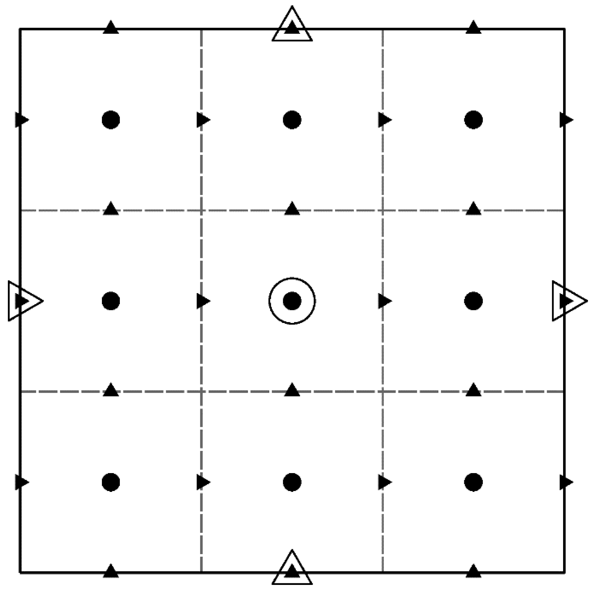
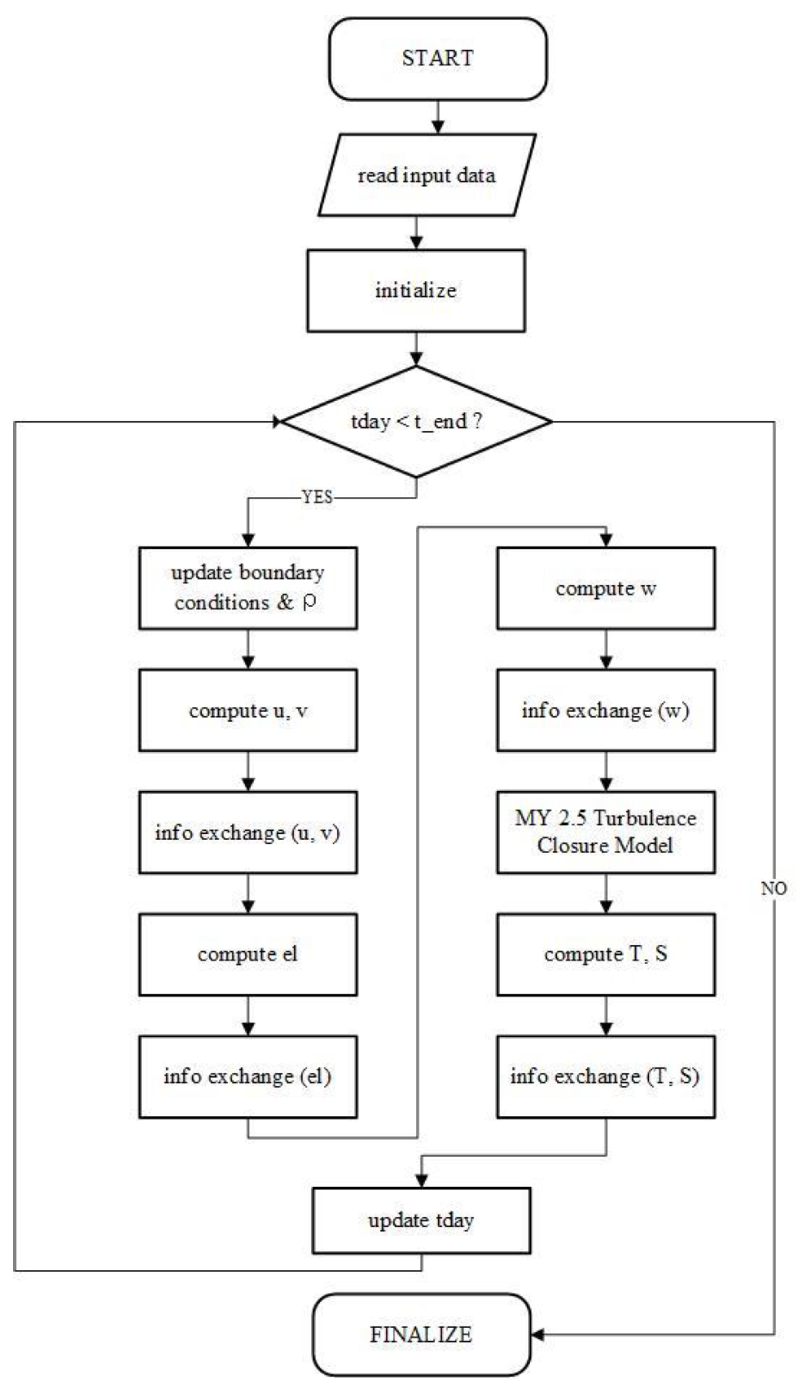
2.1. Basic Model Characteristics

Under the hydrostatic assumption and the Boussinesq approximation, we introduce a horizontal non-orthogonal curvilinear coordinate transformation ($\xi =\xi \left(x,y\right)$, $\eta =\eta \left(x,y\right)$) and a vertical $\sigma$ coordinate transformation ($\sigma =\frac{z-\zeta }{H+\zeta }$, $\sigma$ varies from −1 at $z=-H$ to 0 at $z=\zeta$) to the primitive equations to form the basis of this model. The governing equations are first derived by Chen et al. [45]. The momentum equations are given as

$$\frac{\partial DJ{u}_1}{\partial t}+\frac{\partial DJ\widehat{U}{u}_1}{\partial \xi }+\frac{\partial DJ\widehat{V}{u}_1}{\partial \eta }+\frac{\partial J\omega u_1}{\partial \sigma }-D{h}_2\widehat{V}\left[v_1\frac{\partial }{\partial \xi }\left(\frac{J}{h_1}\right)-u_1\frac{\partial }{\partial \eta }\left(\frac{J}{h_2}\right)+Jf\right]-D{h}_2{u}_1{v}_1\frac{\partial }{\partial \xi }\left(\frac{h_3}{h_1{h}_2}\right)=-h_{2}gD\frac{\partial \zeta }{\partial \xi }+\frac{g{h}_{2}D}{{\rho }_0}\frac{\partial D}{\partial \xi }{{\displaystyle \int }}_{\sigma }^0\sigma \frac{\partial \rho }{\partial \sigma }d\sigma -\frac{g{h}_2{D}^2}{{\rho }_0}\frac{\partial }{\partial \xi }{{\displaystyle \int }}_{\sigma }^0\rho d\sigma +\frac{1}{D}\frac{\partial }{\partial \sigma }\left(K_m\frac{\partial J{u}_1}{\partial \sigma }\right)+DJ{F}_x;$$

(1)

$$\frac{\partial DJ{v}_1}{\partial t}+\frac{\partial DJ\widehat{U}{v}_1}{\partial \xi }+\frac{\partial DJ\widehat{V}{v}_1}{\partial \eta }+\frac{\partial J\omega v_1}{\partial \sigma }-D{h}_1\widehat{U}\left[v_1\frac{\partial }{\partial \xi }\left(\frac{J}{h_1}\right)-u_1\frac{\partial }{\partial \eta }\left(\frac{J}{h_2}\right)+Jf\right]-D{h}_1{u}_1{v}_1\frac{\partial }{\partial \eta }\left(\frac{h_3}{h_1{h}_2}\right)=-h_{1}gD\frac{\partial \zeta }{\partial \xi }+\frac{g{h}_{1}D}{{\rho }_0}\frac{\partial D}{\partial \eta }{{\displaystyle \int }}_{\sigma }^0\sigma \frac{\partial \rho }{\partial \sigma }d\sigma -\frac{g{h}_1{D}^2}{{\rho }_0}\frac{\partial }{\partial \eta }{{\displaystyle \int }}_{\sigma }^0\rho d\sigma +\frac{1}{D}\frac{\partial }{\partial \sigma }\left(K_m\frac{\partial J{v}_1}{\partial \sigma }\right)+DJ{F}_y,$$

(2)

and the continuity equation is

$$\frac{\partial \mathsf{\zeta }}{\partial \mathrm{t}}+\frac{1}{J}\left[\frac{\partial }{\partial \xi }\left(DJ\widehat{U}\right)+\frac{\partial }{\partial \eta }\left(DJ\widehat{V}\right)\right]+\frac{\partial \omega }{\partial \sigma }=0,$$

(3)

where

$$\omega =w-\sigma \left(\widehat{U}\frac{\partial D}{\partial \xi }+\widehat{V}\frac{\partial D}{\partial \eta }\right)-\left[\left(1+\sigma \right)\frac{\partial \mathsf{\zeta }}{\partial \mathrm{t}}+\widehat{U}\frac{\partial \mathsf{\zeta }}{\partial \mathsf{\xi }}+\widehat{V}\frac{\partial \mathsf{\zeta }}{\partial \eta }\right].$$

(4)

The conservation equation for salinity and temperature can be written as

$$\frac{\partial JDS}{\partial t}+\frac{\partial JD\widehat{U}S}{\partial \xi }+\frac{\partial JD\widehat{V}S}{\partial \eta }+\frac{\partial J\omega S}{\partial \sigma }=\frac{1}{D}\frac{\partial }{\partial \sigma }\left(K_h\frac{\partial JS}{\partial \sigma }\right)+DJ{F}_s,$$

(5)

$$\frac{\partial JD\theta }{\partial t}+\frac{\partial JD\widehat{U}\theta }{\partial \xi }+\frac{\partial JD\widehat{V}\theta }{\partial \eta }+\frac{\partial J\omega \theta }{\partial \sigma }=\frac{1}{D}\frac{\partial }{\partial \sigma }\left(K_h\frac{\partial J\theta }{\partial \sigma }\right)+DJ{F}_{\theta }.$$

(6)

The density equation is

$${\rho }_{total}={\rho }_{total}\left(\theta ,S\right),$$

(7)

where

$${\rho }_{total}=\rho +{\rho }_0.$$

(8)

In the above equations, $H$ is the water depth, and $D=H+\zeta$ with $\zeta$, the surface elevation.$f$ is the Coriolis parameter, and $g$ is the gravitational acceleration. $J$ is the Jacobian function, which can be calculated by $J=x_{\xi }{y}_{\eta }-x_{\eta }{y}_{\xi }$, where the subscripts indicate partial derivatives. $h_1$, $h_2$, and $h_3$ are defined as

$$h_1=\sqrt{x_{\xi }^2+y_{\xi }^2}, h_2=\sqrt{x_{\eta }^2+y_{\eta }^2}, h_3=y_{\xi }{y}_{\eta }+x_{\xi }{x}_{\eta }.$$

(9)

$u_1$ and $v_1$ are the $\xi$ and $\eta$ components of the velocity, respectively, and the relationship between them and the x and y components ($u$ and $v$) is

$$u_1=\frac{h_2}{J}\left(x_{\xi }u+y_{\xi }v\right), v_1=\frac{h_1}{J}\left(x_{\eta }u+y_{\eta }v\right).$$

(10)

$\widehat{U}$ and $\widehat{V}$ are defined as

$$\widehat{U}=\frac{1}{J}(h_2{u}_1-\frac{h_3}{h_1}{v}_1),\widehat{V}=\frac{1}{J}(h_1{v}_1-\frac{h_3}{h_2}{u}_1).$$

(11)

In Equations (5) and (6), $S$ is the salinity and $\theta$ is the potential temperature; $\rho$ and ${\rho }_0$ are the perturbation and reference densities; the vertical eddy viscosity coefficient and the thermal vertical eddy diffusion coefficient are denoted as $K_m$ and $K_h$, and the modified Mellor–Yamada level 2.5 turbulence closure scheme [46,47] is applied to calculate them; $F$ represents the horizontal diffusion terms, which can be expressed as

$$F_{\xi }=\frac{\partial }{\partial \xi }\left(2A_m\frac{h_2}{h_1}\frac{\partial u_1}{\partial \xi }\right)+\frac{\partial }{\partial \eta }\left(A_m\left(\frac{h_1}{h_2}\frac{\partial u_1}{\partial \eta }+\frac{\partial v_1}{\partial \xi }\right)\right);$$

(12)

$$F_{\eta }=\frac{\partial }{\partial \xi }\left(A_m\left(\frac{\partial u_1}{\partial \eta }+\frac{h_2}{h_1}\frac{\partial v_1}{\partial \xi }\right)\right)+\frac{\partial }{\partial \eta }\left(2A_m\frac{h_1}{h_2}\frac{\partial v_1}{\partial \eta }\right);$$

(13)

$$F_S=\frac{\partial }{\partial \xi }\left(A_h\frac{h_2}{h_1}\frac{\partial S}{\partial \xi }\right)+\frac{\partial }{\partial \eta }\left(A_h\frac{h_1}{h_2}\frac{\partial S}{\partial \eta }\right);$$

(14)

$$F_{\theta }=\frac{\partial }{\partial \xi }\left(A_h\frac{h_2}{h_1}\frac{\partial \theta }{\partial \xi }\right)+\frac{\partial }{\partial \eta }\left(A_h\frac{h_1}{h_2}\frac{\partial \theta }{\partial \eta }\right),$$

(15)

where $A_m$ and $A_h$ are the horizontal counterparts of $K_m$ and $K_h$, respectively, and are obtained by Smagorinsky’s formula [48].

The initial elevation and water current are usually set to zero, and the initial salinity and temperature filed are interpolated from climatological or observational data.

The surface and bottom boundary conditions for the momentum, salinity, and temperature equations are given by

$$\omega {│}_{\sigma =0 or-1}=0;$$

(16)

$$\frac{{\rho }_0{K}_m}{D}\left(\frac{\partial u_1}{\partial \sigma }, \frac{\partial v_1}{\partial \sigma }\right){│}_{\sigma =0}=\left({\tau }_{0\xi }, {\tau }_{0\eta }\right),\frac{{\rho }_0{K}_m}{D}\left(\frac{\partial u_1}{\partial \sigma }, \frac{\partial v_1}{\partial \sigma }\right){│}_{\sigma =-1}=\left({\tau }_{b\xi }, {\tau }_{b\eta }\right);$$

(17)

$$\frac{{\rho }_0{K}_h}{D}\frac{\partial S}{\partial \sigma }{│}_{\sigma =0}=P_{net},\frac{{\rho }_0{K}_h}{D}\frac{\partial S}{\partial \sigma }{│}_{\sigma =-1}=0;$$

(18)

$$\frac{{\rho }_0{K}_h}{D}\frac{\partial \theta }{\partial \sigma }{│}_{\sigma =0}=Q_{net},\frac{{\rho }_0{K}_h}{D}\frac{\partial \theta }{\partial \sigma }{│}_{\sigma =-1}=0.$$

(19)

In Equation (17), $\left({\tau }_{0\xi }, {\tau }_{0\eta }\right)$ are the $\xi$ and $\eta$ components of surface wind stresses, which are calculated with the neutral steady-state drag coefficient [49]. $\left({\tau }_{b\xi }, {\tau }_{b\eta }\right)$ are the $\xi$ and $\eta$ components of bottom stresses, and they can be obtained with the following formula:

$$\left({\tau }_{b\xi }, {\tau }_{b\eta }\right)=C_d\sqrt{u_1^2+v_1^2}\cdot \left(u_1, v_1\right),$$

(20)

where $C_d$ is the bottom drag coefficient which can be determined by the logarithmic law [50]. $P_{net}$ and $Q_{net}$ are the surface net heat and salinity flux, respectively.

The lateral boundary conditions for closed basins are specified as

$$v_t=0,$$

(21)

$$v_n=0,$$

(22)

$$\frac{\partial S}{\partial n}=0,$$

(23)

$$\frac{\partial \theta }{\partial n}=0,$$

(24)

where $t$ and $n$ represent the tangential and normal direction to the boundary, respectively.

The open boundary conditions are yielded by measured data or radiation boundary conditions.

The governing equations are discretized using the finite difference method on an Arakawa C-grid [51] (Figure 1). The fractional-step method [52] is applied to the time integration of the discretized momentum equations. In the first step, all the terms except for the vertical diffusion terms are treated explicitly with the simple Euler scheme. In the second step, the implicit treatment of the vertical diffusion terms leads to a tri-diagonal matrix, which can be solved by the tri-diagonal matrix algorithm [53], and after that, the horizontal velocity field is obtained. The water elevation is calculated by substituting the n+1 step $u$ and $v$ into the continuity equation. An HSIMT-TVD (high-order spatial interpolation at the middle temporal level coupled with a TVD limiter) scheme with high-order accuracy and non-oscillation is utilized to solve the advection terms in the tracer equations [41].

2.2. Implementation of Nesting

For most of the nested structure-grid models, the nesting procedure is implemented by running multiple models [40], which means the HRG model is driven by the boundary conditions interpolated from the CRG solution and meanwhile, the CRG model is affected by the HRG solution through updating at the nesting interfaces. Associated with mesh refinement, time refinement is usually adopted. The time integration of different-resolution-mesh models will be coupled like the treatment of split-explicit models to the barotropic mode and baroclinic mode. Hence, the nesting algorithm can be simplified as follows:

• Step the CRG model forward to the next time step.
• Interpolate the HRG boundary conditions from the CRG model values both spatially and temporally. The time refinement and spatial refinement usually share the same ratio.
• Step the HRG model forward to the same physical time as the CRG model.
• Update the values of the overlapped CRG points with the new HRG model values.

UFDECOM does not adopt any time-splitting method, and our aim is to run one multi-scale model for better consistency. The grid can be as concise as those used by unstructured-grid models (Figure 2). However, for the numerical integration on one certain grid cell at the nesting interfaces, values of neighboring cells cannot be directly used due to different spatial resolutions. Thus, the virtual-grid method is devised to solve this problem. Figure 2 is a schematic of the virtual-grid method. To put it simply, we set some extra grids next to the nesting interfaces in both horizontal directions. The number of circles in one virtual grid depends on the numerical schemes (it is 4 for the HSIMT-TVD advection scheme). Variables at these grids are obtained not by calculating but by interpolating or updating, so we name them virtual grids. When a virtual grid is used by a finer actual grid, it is an external virtual grid. Otherwise, it is internal. In the numerical integration, if some variable is stepped to the nest time step, the values of virtual grids are interpolated/updated immediately by an information-exchanging subroutine. Therefore, values of actual and virtual grids are renewed almost synchronously and solutions can be obtained in the whole model domain.

Combining the numerical scheme and the virtual-grid method, the general algorithm of UFDECOM is illustrated in a flow diagram (Figure 3). The information-exchanging subroutine is inserted between any two independent processes.

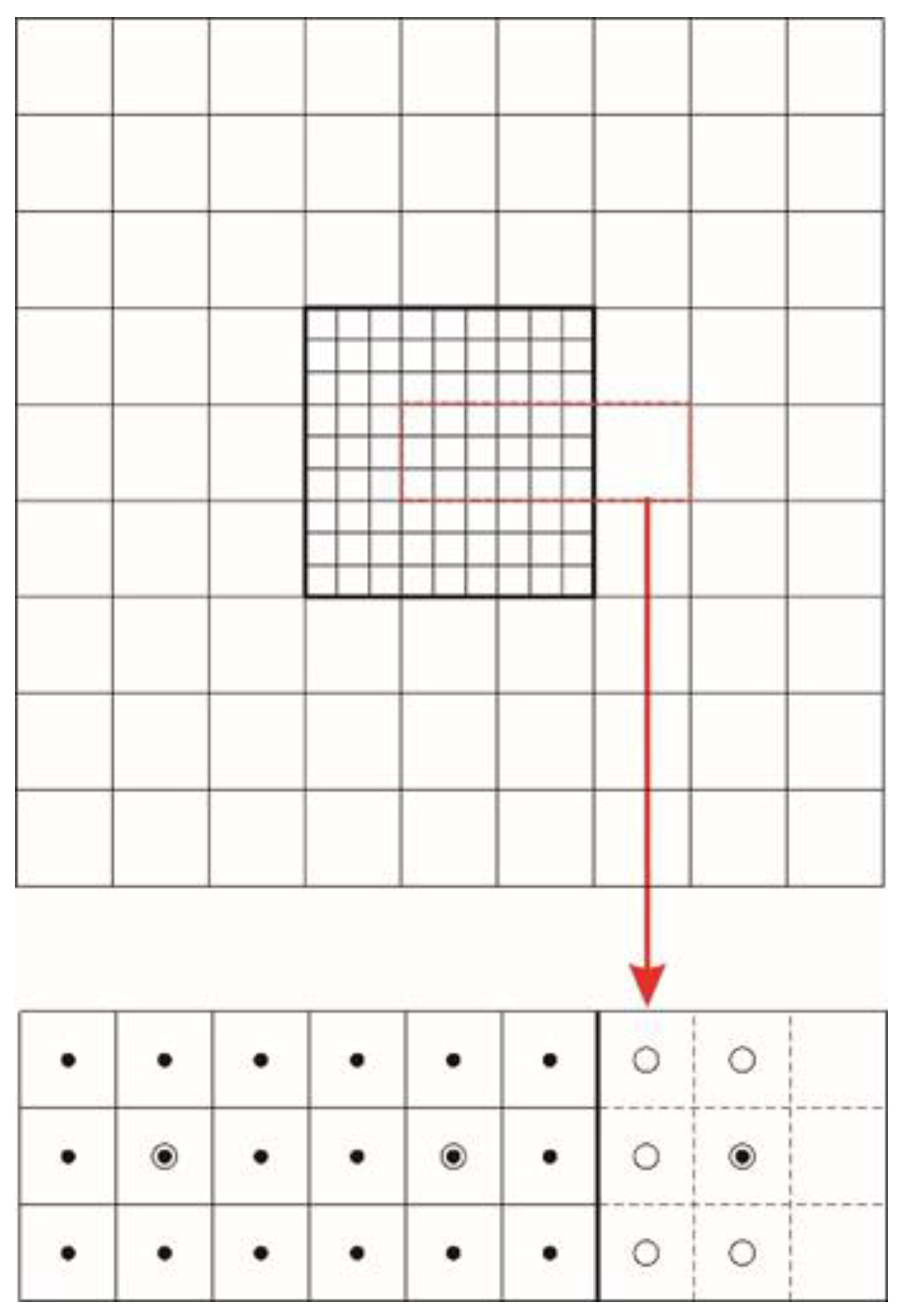
2.3. Embedding Techniques

Obviously, update and interpolation schemes are the most crucial techniques for nested grid models. However, the embedding procedure of updating and interpolating may cause some other problems, which can affect the accuracy, stability, and conservation of solution, and requires careful treatment.

2.3.1. Update Schemes

Since update is feeding the HRG solutions back to the CRG variables, a natural principle will be maximizing the information well revolved on the CRG and damp the small scales as strongly as possible at the same time.

We tested five update schemes in UFDECOM. Here is a brief description.

• Directly-replacing (DR) scheme

In this scheme, all internal-virtual-grid (IVG) variables are directly replaced by the values of their respective nearest actual-grid (AG) points. This scheme is extremely simple and holds no smoothing or conservative characteristics, which shows great instability in our ideal experiments.

2.

Inverse distance weighting interpolation (IDWI) scheme

A certain IVG point is taken as the origin, and we search for its closest AG point in four quadrants. Then, the value is calculated with a weighted average of these four points. This scheme can be expressed as

$${\varphi }^{IVG}=\frac{{\sum }_{i=1}^4{m}_i{w}_i{\varphi }_i^{AG}}{{\sum }_i^4{m}_i{w}_i},$$

(25)

where

$$w_i=\frac{1000}{d_i}.$$

(26)

${\varphi }^{IVG}$ is the value at the IVG point and ${\varphi }_i^{AG}$ is the value at the closest AG point in quadrant i. $m_i$ is the free surface mask, which is updated at each time step. The weight is denoted as $w_i$, which is determined by the distance $d_i$ between ${\varphi }_i^{AG}$ and ${\varphi }^{IVG}$.

• Area-averaging (AVE) scheme

The coarse IVG value in the cell is replaced by the area-weighted sum of the AG values in the same cell

$${\varphi }^{\mathrm{IVG}}=\frac{{{\displaystyle \sum }}_{i=1}^n{A}_i{\varphi }_i^{AG}}{{{\displaystyle \sum }}_{i=1}^n{A}_i},$$

(27)

where A is the area of the fine AG cell and n is the total number of AG cells in the coarse cell.

2.

9-point Shapiro filtering (SF) scheme

The 9-point Shapiro filtering scheme is derived by Shapiro [54]. The transfer function in 2D is presented here:

$${\varphi }^{IVG}={\left(1-S\right)}^2{\varphi }_{i,j}^{AG}+\frac{S}{2}\left(1-S\right)\left({\varphi }_{i-1,j}^{AG}+{\varphi }_{i,j+1}^{AG}+{\varphi }_{i+1,j}^{AG}+{\varphi }_{i,j-1}^{AG}\right)+\frac{S^2}{4}\left({\varphi }_{i-1,j+1}^{AG}+{\varphi }_{i+1,j+1}^{AG}+{\varphi }_{i+1,j-1}^{AG}+{\varphi }_{i-1,j-1}^{AG}\right),$$

(28)

where $S$ is the smoothing element, which is 0.5 in UFDECOM.

3.

Full-weighting operator (FWO) scheme

Debreu, Marchesiello, Penven, and Cambon [36] discovered that using a larger stencil can construct higher-order restriction operators, so they expanded the stencil to 25 points and derive the full-weighting operator scheme. The 2D transfer function is given as

$$\begin{array}{c}{\varphi }^{IVG}={\left(1-S\right)}^2{\varphi }_{i,j}^{AG}+\frac{S}{3}\left(1-S\right)\left({\varphi }_{i-1,j}^{AG}+{\varphi }_{i,j+1}^{AG}+{\varphi }_{i+1,j}^{AG}+{\varphi }_{i,j-1}^{AG}\right)+\frac{S}{6}\left(1-S\right)\left({\varphi }_{i-2,j}^{AG}+{\varphi }_{i,j-2}^{AG}+{\varphi }_{i+2,j}^{AG}+{\varphi }_{i,j+2}^{AG}\right)+\\ \frac{S^2}{9}\left({\varphi }_{i-1,j-1}^{AG}+{\varphi }_{i-1,j+1}^{AG}+{\varphi }_{i+1,j-1}^{AG}+{\varphi }_{i+1,j+1}^{AG}\right)+\frac{S^2}{18}({\varphi }_{i-1,j-2}^{AG}+{\varphi }_{i-1,j+2}^{AG}+{\varphi }_{i+1,j-2}^{AG}+{\varphi }_{i+1,j+2}^{AG}+\\ {\varphi }_{i-2,j-1}^{AG}+{\varphi }_{i-2,j+1}^{AG}+{\varphi }_{i+2,j-1}^{AG}+{\varphi }_{i+2,j+1}^{AG})+\frac{S^2}{36}\left({\varphi }_{i-2,j-2}^{AG}+{\varphi }_{i-2,j+2}^{AG}+{\varphi }_{i+2,j-2}^{AG}+{\varphi }_{i+2,j+2}^{AG}\right),\end{array}$$

(29)

where $S=2/3$.

Among all the update schemes above, the directly-replacing scheme and inverse distance weighting interpolation scheme have low-order accuracy and are coded only for possible tests at the early developing stage, while the area-averaging scheme and 9-point Shapiro filtering scheme have been widely used and tested by nested grid models [33,34,35,36,55,56]. Debreu, Marchesiello, Penven, and Cambon [36] used a larger stencil to develop the high-order full-weighting operator scheme, which were designed to properly damp subgrid scale features. On the contrary, the area-averaging scheme and the Shapiro-filtering scheme require artificial increasing diffusion near the nesting interfaces (sponge layer) to damp the small-scale modes. Ideal experiments indicated that the full-weighting operator could yield a significant improvement over the solution based on the area-averaging scheme [36]. So further experiments in this work adopted the full-weighting operator scheme as the update scheme considering previous research.

2.3.2. Interpolation Schemes

In contrast to update schemes, plenty of interpolation schemes have been used in nested grid models [33]. Modelers have been seeking a high-order interpolation scheme, which is meanwhile conservative. High-order interpolation schemes may produce spurious oscillations especially in areas of sharp gradients [57]. UFDECOM has seven available options.

• Zeroth-order uniform interpolation (UNI) scheme

All external virtual grid (EVG) points within an AG cell are assigned the same value of that cell.

2.

Inverse distance weighting interpolation (IDWI) scheme

It is the same scheme as the IDWI update scheme.

3.

Inverse bilinear interpolation (IBI) scheme

In this scheme, an EVG point value is interpolated in a quadrilateral defined by four surrounding AG points. We choose the inverse bilinear interpolation scheme, which applies to a random quadrilateral, in case that the nested grid has an even refinement ratio.

4.

Quadratic interpolation (QI) scheme

Clark and Farley [55] developed this scheme based on the conservation relation suggested by Kurihara et al. [58]. One is referred to Clark and Farley [55] for detailed expressions.

5.

HSIMT parabolic interpolation (HPI) scheme

A key issue in the construction of a flux-based advection scheme is to determine the flux at the cell interface, while this problem reduces to estimating the concentration of some specific substance ($\varphi$) for a C-grid based model. In the HSIMT-TVD scheme, an upwind parabola function is used to describe the distribution of $\varphi$, which inspires us to apply the same method to interpolating the values of external virtual points. This idea can maintain the consistency of variable distribution for both actual grids and virtual grids. Following the expressions of Wu and Zhu [41], the local distribution is in the form of

$$f\left(\xi \right)=b{\xi }^2+c\xi +d,$$

(30)

where $\xi =\mathsf{\epsilon }+1/2$ and $\epsilon$ is the normalized local coordinate, which varies from −1 on ${\varphi }_{i-1}^{AG}$ to 1 on ${\varphi }_{i+1}^{AG}$. If $u_i^{AG}\ge 0$, the three coefficients will be as follows

$$\{\begin{array}{l}b=\frac{1}{2}{\Delta }_{i-\frac{1}{2}}-\frac{1}{2}{\Delta }_{i-\frac{3}{2}}\\ c={\Delta }_{i-\frac{1}{2}}\\ d=\frac{1}{3}{\Delta }_{i-\frac{1}{2}}+\frac{1}{6}{\Delta }_{i-\frac{3}{2}}+{\varphi }_{i-1}^{AG}\end{array}.$$

(31)

Under the opposite condition, the expressions will be

$$\{\begin{array}{l}b=\frac{1}{2}{\Delta }_{i+\frac{1}{2}}-\frac{1}{2}{\Delta }_{i-\frac{1}{2}}\\ c={\Delta }_{i-\frac{1}{2}}\\ d=-\frac{1}{6}{\Delta }_{i+\frac{1}{2}}-\frac{1}{3}{\Delta }_{i-\frac{1}{2}}+{\varphi }_i^{AG}\end{array},$$

(32)

where ${\Delta }_{i-\frac{1}{2}}={\varphi }_i^{AG}-{\varphi }_{i-1}^{AG}$.

The basic idea of the HPI scheme is actually originated from the piecewise parabolic assumption in the piecewise parabolic method (PPM) [59]. The PPM is a higher-order extension of Godunov’s method [60,61], which is of a type first introduced by van Leer in his MUSCL algorithm [62]. The MUSCL algorithm was devised to construct a numerical scheme for solving the advection terms in the trace equations, while the HSIMT parabolic scheme is developed for information exchange in the nested grid model. Thus, the MUSCL algorithm and the HSIMT parabolic scheme serve for totally different purposes. Generally speaking, the HSIMT parabolic scheme can be seen as a transplantation of a high-order version the MUSCL approach to the nested grid model. However, nested grid model with such upwind piecewise parabolic interpolation scheme has been unseen in previous research.

6.

Upwind advection-equivalent interpolation (AEI) scheme

The basic idea of the AEI scheme is to design a shape-preserving interpolator from a variety of monotone advection algorithms [63]. Thus, a formal equivalence of the advection scheme and interpolator can be obtained on discrete meshes. Starting from an advection scheme formula, the local Courant number vector is replaced by a normalized local coordinate whose origin coincides with the center of a coarse AG cell (for scalar variables). The accuracy of the derived interpolation scheme is maintained the same as that of the advection scheme utilized.

The upwind AEI scheme here is a little different from that described by Alapaty, Mathur, and Odman [57]. The original AEI scheme based on the upwind advection scheme is actually the same as the linear interpolation. We make it upwind physically by retaining the velocity sign in the formula. The scheme in 1D can be expressed as

$${\varphi }^{EVG}={\varphi }_i^{AG}+\frac{\left|u_i\right|+u_i}{2\left|u_i\right|}\epsilon \left({\varphi }_i^{AG}-{\varphi }_{i-1}^{AG}\right)+\frac{\left|u_i\right|-u_i}{2\left|u_i\right|}\epsilon \left({\varphi }_{i+1}^{AG}-{\varphi }_i^{AG}\right).$$

(33)

7.

HSIMT advection-equivalent interpolation scheme

Since the advection scheme adopted by UFDECOM is the HSIMT-TVD scheme, a natural idea is to develop a desirable AEI scheme from this robust advection scheme. One can refer to the paper of Wu and Zhu [41] for the derivation and details of this flux-based advection scheme. We omit the derivation process and directly give the final formulae. The HSIMT AEI scheme can be obtained by replacing $-u\Delta t/\Delta X$ by $\epsilon$ to yield the following

$${\varphi }^{EVG}={\varphi }_i^{AG}+\epsilon \left({\varphi }_{i+\frac{1}{2}}-{\varphi }_{i-\frac{1}{2}}\right),$$

(34)

where

$${\varphi }_{i-\frac{1}{2}}={\varphi }_{i-1}^{AG}+0.5\left[\left(-\frac{1}{4}{\kappa }_{i-\frac{1}{2}}+\frac{1}{2}+\frac{1}{12}\frac{1}{{\kappa }_{i-\frac{1}{2}}}\right)\frac{{\Delta }_{i-\frac{3}{2}}}{{\Delta }_{i-\frac{1}{2}}}+\left(\frac{1}{4}{\kappa }_{i-\frac{1}{2}}+\frac{1}{2}-\frac{1}{12}\frac{1}{{\kappa }_{i-\frac{1}{2}}}\right)\right]{\kappa }_{i-\frac{1}{2}}{\Delta }_{i-\frac{1}{2}}$$

(35)

when $u_i^{AG}\ge 0$, or

$${\varphi }_{i-\frac{1}{2}}={\varphi }_i^{AG}-0.5\left[\left(-\frac{1}{4}{\kappa }_{i-\frac{1}{2}}+\frac{1}{2}+\frac{1}{12}\frac{1}{{\kappa }_{i-\frac{1}{2}}}\right)\frac{{\Delta }_{i+\frac{1}{2}}}{{\Delta }_{i-\frac{1}{2}}}+\left(\frac{1}{4}{\kappa }_{i-\frac{1}{2}}+\frac{1}{2}-\frac{1}{12}\frac{1}{{\kappa }_{i-\frac{1}{2}}}\right)\right]{\kappa }_{i-\frac{1}{2}}{\Delta }_{i-\frac{1}{2}}$$

(36)

otherwise. In Equations (35) and (36), ${\kappa }_{i-\frac{1}{2}}=1-\left|\epsilon \right|$ and ${\mathsf{\Delta }}_{\mathrm{i}-\frac{1}{2}}={\varphi }_i^{AG}-{\varphi }_{i-1}^{AG}$.

2.3.3. Conservation

If numerical schemes are written in flux form, conservation is maintained in a structured grid model. However, this property vanishes for two-way interactive nested models because of the unavoidable mismatch of fluxes between different-resolution grids at nested interfaces. Although enforced conservation can cause problems on computational accuracy and stability, it is required for long-term integrations. A flux correction algorithm [36,64,65] is applied for volume and tracer conservation. Its basic idea is to integrate the coarse grid variables using the summations of the HRG fluxes at the nested interfaces.

3. Ideal Salinity Advection Experiment

The HPI scheme and HSIMT AEI scheme described above are evaluated here using an idealized salinity advection test case. The experiment design imitates the test problem used to compare different spatial interpolation schemes in nested grid models in Alapaty, Mathur, and Odman [57].

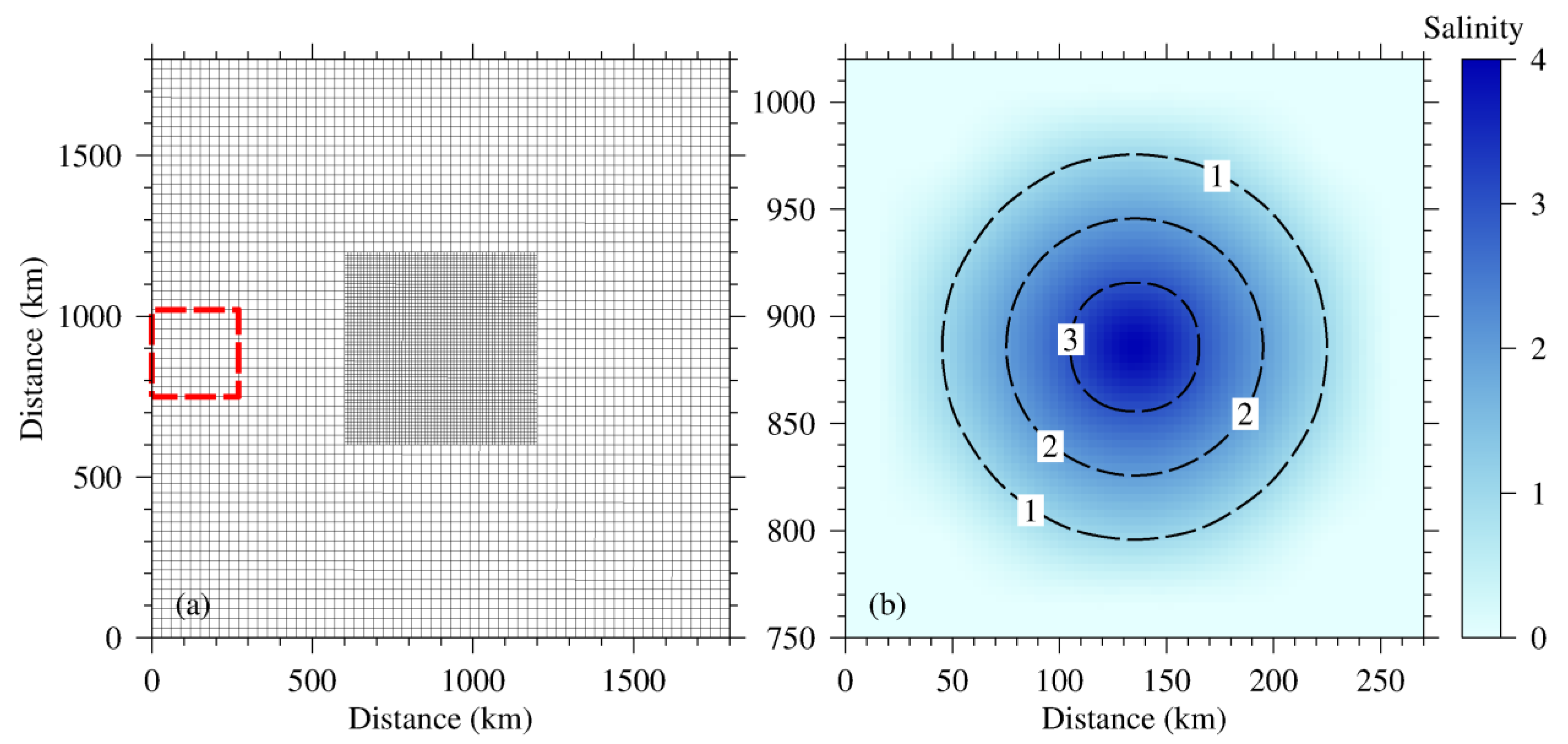
3.1. Experiment Design

Three grids are involved in the ideal experiment. A coarse grid has 60 × 60 cells with a resolution of 30 km, and a fine grid consists of 180 × 180 cells with a resolution of 10 km. The nested grid is produced by refining the central square area of the coarse grid with a refinement ratio of 3 (Figure 4a). The initial salinity field consists of a cylindrical distribution with a radius of four coarse-grid cells near the west boundary of the whole numerical domain. The salinity decreases linearly from 4 psu in the center to 0 psu on the edge (Figure 4b). The uniform eastward 1 m/s flow is specified as the background hydrodynamic condition, and the friction as well as the horizontal/vertical mixing are excluded. Thus, numerical integrations are only determined by the advection terms in the salinity equation. Four simulations which applied the Upwind AEI scheme, QI scheme, HPI scheme, and HSIMT AEI scheme as the interpolation scheme are conducted on the nested grid. Meanwhile, two more numerical cases run on the two structured grids are used to be compared with the nested grid solutions.

3.2. Results and Discussion

The maximum, the minimum, and the sum of the salinity field are used to evaluate the performance of each interpolation scheme. The maximum indicates the peak preservation skill, and the minimum value shows the oscillations introduced by the interpolation process. Total salt of the whole numerical domain can measure the conservation properties of each scheme. Figure 5 illustrates time series of the three indices for all six cases. The saline water mass reaches the western nesting interface at about hour 94, while completely leaves the refined domain at hour 327 approximately. The maximum value declines due to numerical diffusion. However, the CRG case shows a faster decreasing rate than the HRG one because the numerical diffusion is smaller in the HRG than in the CRG. As seen in Figure 5a, the nested grid solutions exhibit strong ability to retain the salinity peak due to the increased resolution after the scalar distribution is advected to the fine-grid subdomain. The two AEI schemes result in an overshoot of the maximum, which is indictive of poor performance of interpolation scheme, whereas the QI scheme and HPI scheme present better continuity during transition from the coarse-grid subdomain to the fine-grid subdomain.

A significant decrease in minimum occurs several hours before the saline water entering the fine-grid subdomain, and the minimum value recovers afterward (Figure 5b). The magnitude of decrease in the HPI case is the smallest and the minimum quickly resumes to zero at hour 110, which suggests that the HPI scheme is the most stable scheme among the four schemes. However, the low-order upwind AEI scheme delivers the worst performance with the minimum falling to nearly −0.07 psu. The domain minimum behaves similarly for the QI scheme and the HSIMT AEI scheme.

Figure 5c presents a comparison of mass conservation properties for each scheme via the temporal variance of relative total salt. The relative total salt undergoes a concave slope because of increased resolution when the saline water mass is entering the fine grid from the coarse grid, and then, it almost remains the same while the salinity distribution is resolved completely in the high-resolution subdomain. A convex variance appears during transition from the fine-grid subdomain to the coarse-grid subdomain. The upwind AEI scheme overpredicted the total salt with a relative value of 100.4%, while on the contrary, the high-order HPI scheme results in an underprediction with a 0.2% deficit. The QI scheme and the HSIMT AEI scheme give more reasonable performances in conserving the total mass compared with the above two schemes.

The differences between the HRG solution and any nested grid solution in the refined subdomain are taken as the absolute errors. Figure 6 illustrates the distribution of absolute errors for each interpolation scheme at hour 212 of simulation (when the saline water mass is at the center of the refined subdomain). For all the interpolation schemes, underpredictions are observed at the center of the distribution, however, overpredictions appear toward both the upwind and downwind edges of the distribution, which can be owed to the numerical diffusion of the advection scheme. The temporal variance of normalized root-mean-square error (NRMSE) is depicted in Figure 7. In fact, four nested-grid simulations show very slight differences between each other in the NRMSE, which is also evidenced by Figure 6.

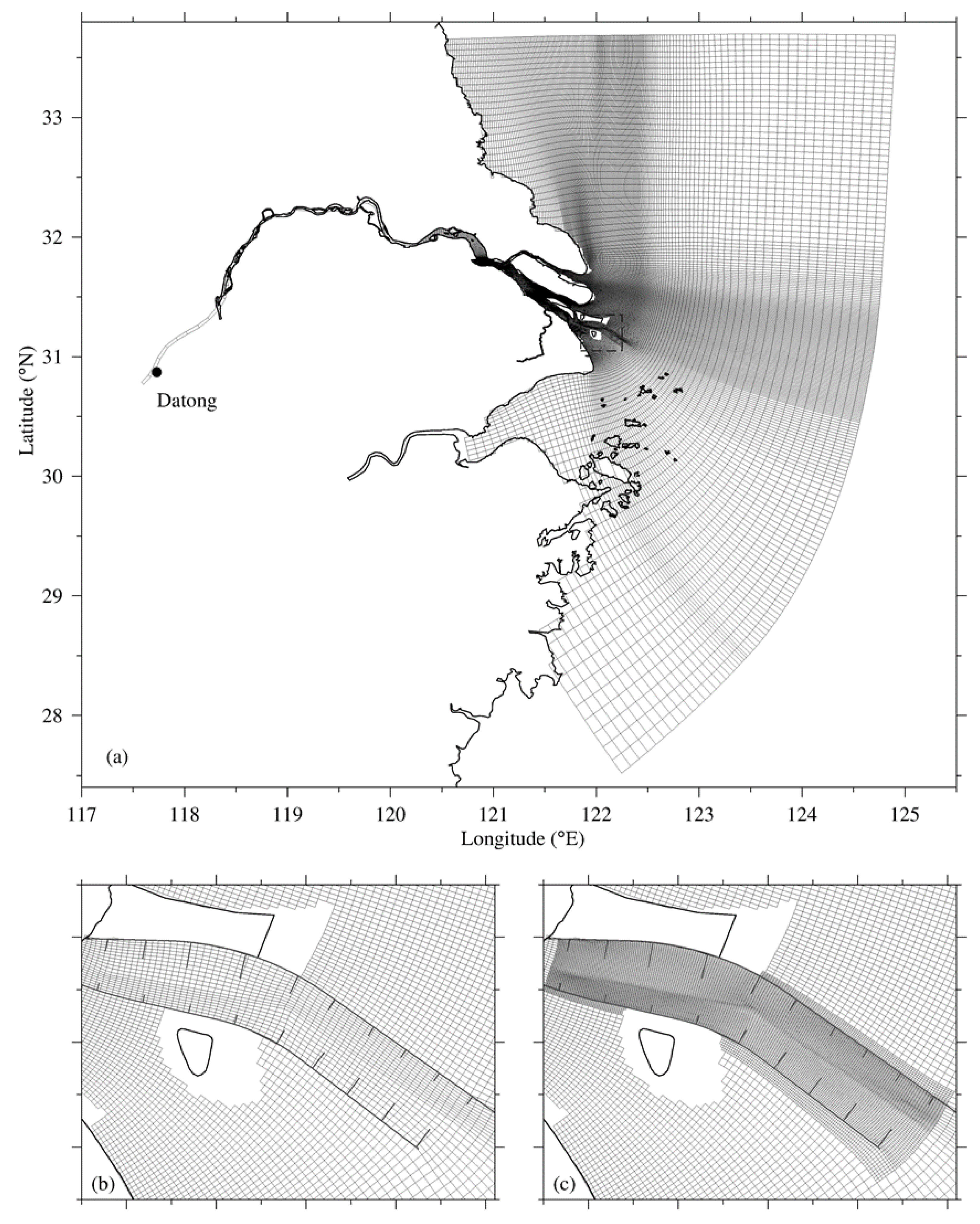
4. Validation and Assessment

The newborn UFDECOM was applied to a realistic case to test its reliability and robustness in this section. The observational data were used to validate the nested model, and the nested solutions were compared with a reference solution obtained on a structured grid to further evaluate different interpolation schemes, in which the HPI scheme and HSIMT AEI scheme are totally original.

4.1. Observational Data

A full description of the measured data can be found in Li et al. [66] and only the necessary information is summarized here. Four synchronous surveys were conducted at three sites (A, B, and C) (Figure 8) in the North Passage of the Changjiang Estuary during four tidal phases, which were the spring tide (16–18 November 2013), the moderate tide after spring tide (MTAS) (20–22 November 2013), the neap tide (24–26 November 2013), and the moderate tide after neap tide (MTAN) (29 November–1 December 2013), respectively. The current and salinity data were adopted for validation.

4.2. Model Configuration & Experiments

The structured grid covers the Changjiang Estuary, and its adjacent seas (Figure 9a), with the minimal cell size reaching nearly 800 × 300 m² in the Deep Waterway Project area (Figure 9b). A part of the mesh covering this area was refined with the ratio of 3 (Figure 9c), and the cells were renumbered to make a new grid file for the calculation of UFDECOM. The models have 10 uniform $\sigma$ layers in the vertical direction.

The tidal constants of 16 astronomical constituents (M₂, S₂, N₂, K₂, K₁, O₁, P₁, Q₁, MU₂, NU₂, T₂, L₂, 2N₂, J₁, M₁, and OO₁), which are derived from the NaoTide dataset (https://www.miz.nao.ac.jp/staffs/nao99/, accessed on 25 September 2019), were utilized to calculate the tidal level as the open boundary elevation. The open boundary condition for salinity was obtained from the monthly mean salinity of a larger domain model [67]. The initial salinity distribution was interpolated from the Ocean Atlas in Huanghai Sea and East China Sea (Hydrology) [68] outside the river mouth and from recently collected field data in the estuary. The daily Changjiang River discharge was measured at the Datong Hydrological Station. The 6-hourly sea surface wind data from the European Center for Medium-Range Weather Forecasts (ECMWF) reanalysis data products with the resolution of 0.125° × 0.125° were used to force the models.

Five experiments were conducted to validate the nested model and assess the performance of four interpolation schemes. A simulation was run on the structured grid in Experiment 0 (Exp. 0) to produce a reference solution, while Experiment 1–4 (Exp. 1–4) were conducted on the nested grid with the FWO scheme as update scheme and four different interpolation schemes, respectively (

Table 1. Interpolation schemes in Exp. 1–4.

Experiment	Interpolation Scheme
Exp. 1	Upwind AEI
Exp. 2	QI
Exp. 3	HPI
Exp. 4	HSIMT AEI

). The flux correction method was applied to the nested grid model. All the simulations started from 1 October 2013 and ran for 70 days.

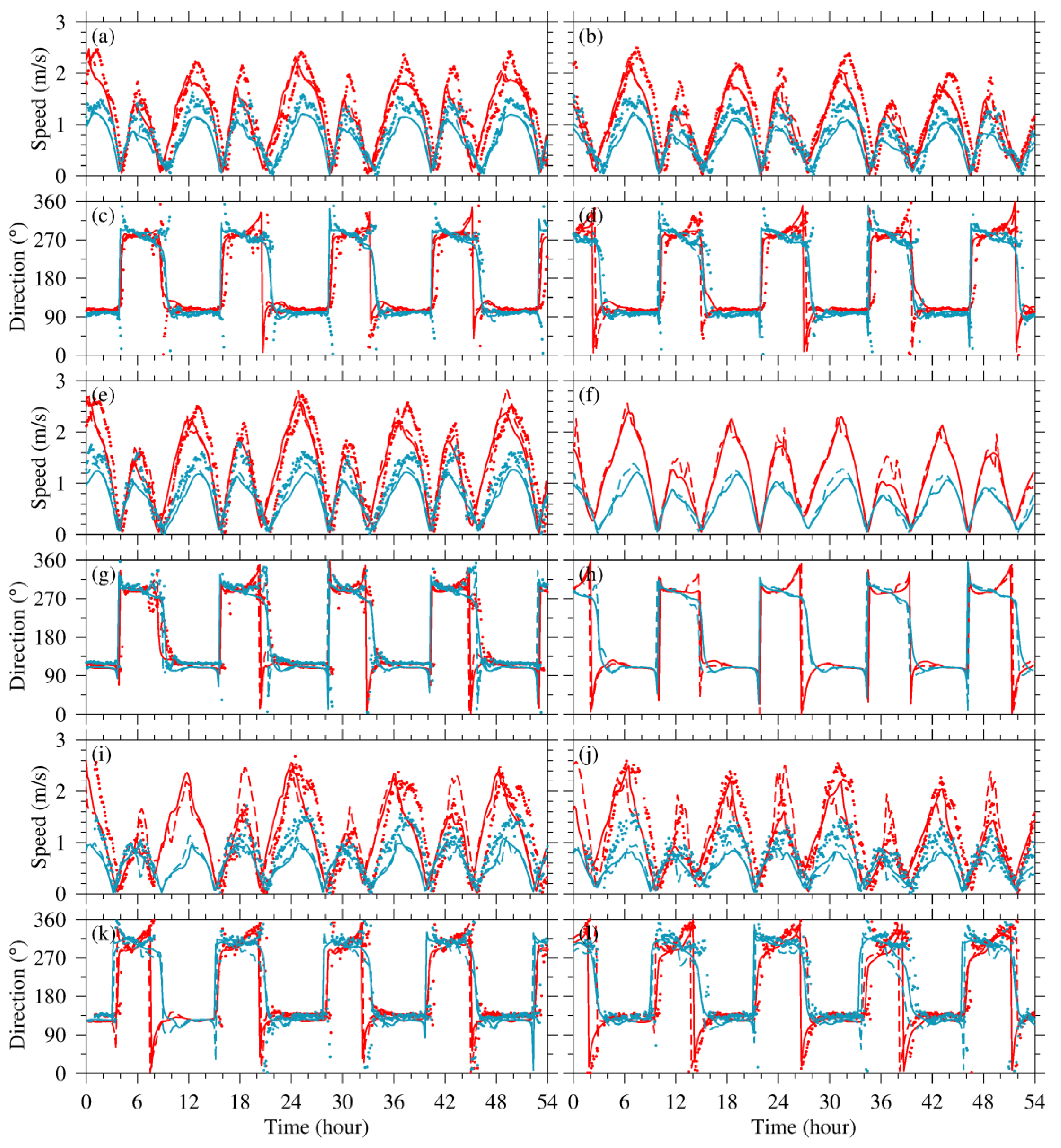
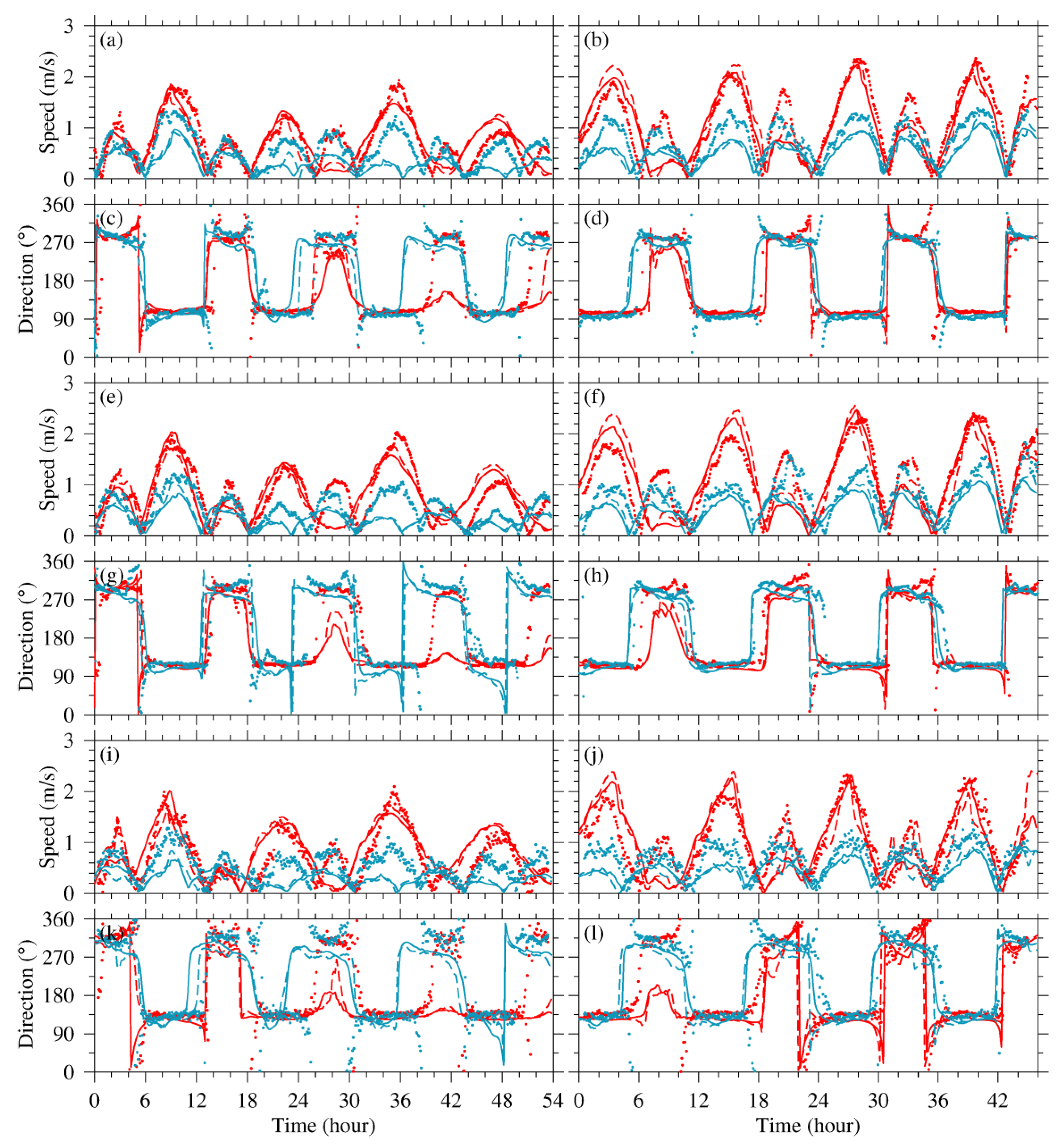
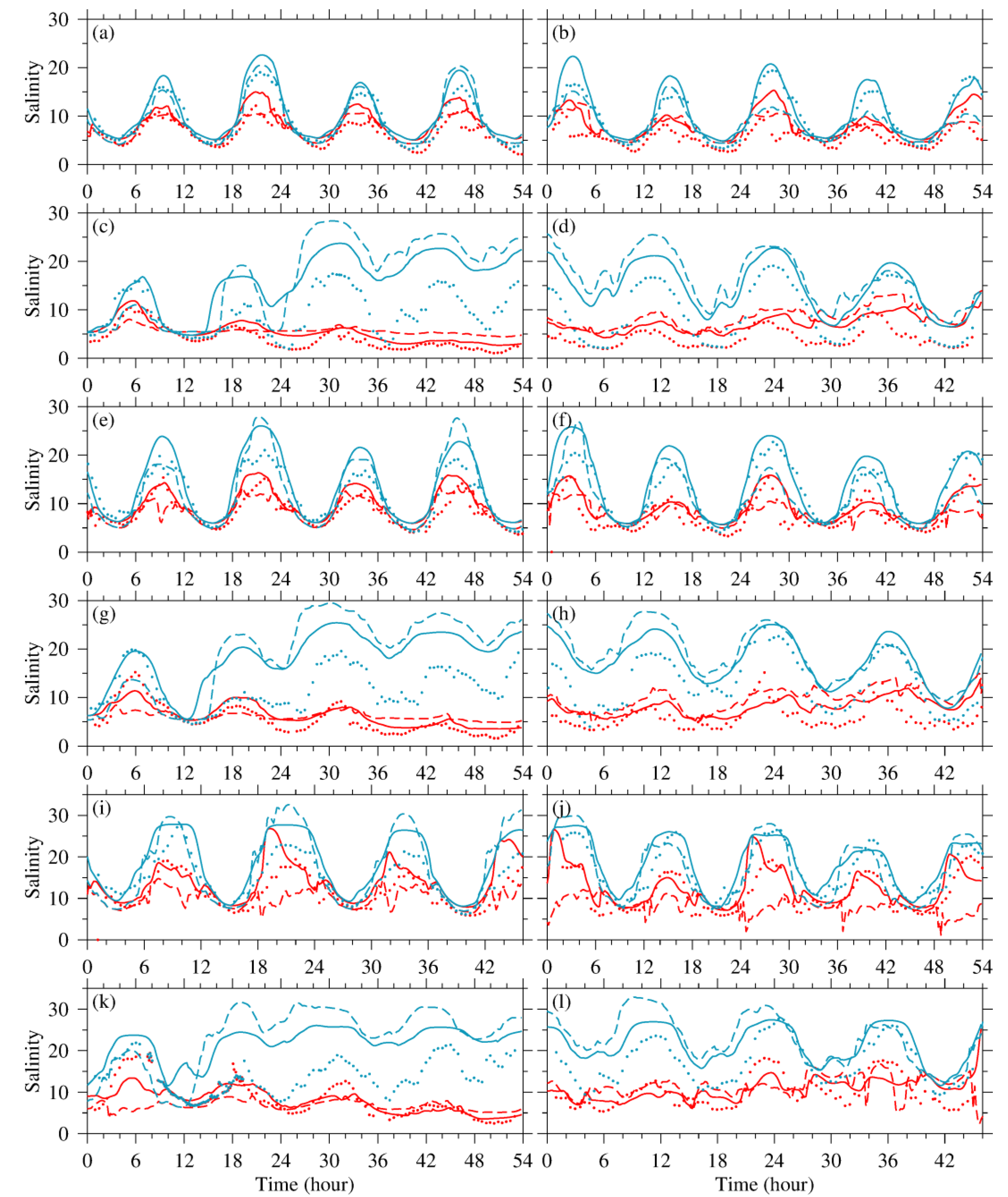
4.3. Validation and Interpolation Scheme Assessment

Performance of the models was quantified by the correlation coefficient (CC), the root-mean-square error (RMSE), and the skill score (SS) [69]. The formulae are given as

$$CC=\frac{{\sum }_{i=1}^N\left(X_{mod}-{\overline{X}}_{mod}\right)\left(X_{obs}-{\overline{X}}_{obs}\right)}{{\left[{\sum }_{i=1}^N{\left(X_{mod}-{\overline{X}}_{mod}\right)}^2{\sum }_{i=1}^N{\left(X_{obs}-{\overline{X}}_{obs}\right)}^2\right]}^{1/2}};$$

(37)

$$RMSE={\left[{\sum }_{i=1}^N{\left(X_{mod}-X_{obs}\right)}^2/N\right]}^{1/2};$$

(38)

$$SS=1-\frac{{\sum }_{i=1}^N{\left(X_{mod}-X_{obs}\right)}^2}{{\sum }_{i=1}^N{\left(X_{obs}-{\overline{X}}_{obs}\right)}^2},$$

(39)

where $X_{mod}$ and $X_{obs}$ are the variables of model results and observational data, respectively, and $\overline{X}$ denotes the time average of the variable. The SS was introduced by [70] as a statistical metric to describe the degree to which the observed deviations from the observed mean correspond to the simulated derivations from the observed mean. Its value ranges from 0 to 1, representing total disagreement to perfect agreement between model results and observational data.

The validation statistics of flow velocity are summarized in

Table 2. Model validation statistics of flow velocity at the observational sites (value at surface layer/value at bottom layer).

Exp.	A			B			C
	CC	RMSE	SS	CC	RMSE	SS	CC	RMSE	SS
Exp. 0	0.85/0.88	0.35/0.29	0.91/0.84	0.84/0.87	0.39/0.31	0.91/0.84	0.79/0.76	0.41/0.32	0.88/0.73
Exp. 1	0.83/0.82	0.39/0.31	0.91/0.82	0.85/0.83	0.44/0.31	0.91/0.84	0.76/0.60	0.46/0.41	0.87/0.62
Exp. 2	0.83/0.83	0.39/0.31	0.91/0.82	0.85/0.84	0.43/0.31	0.91/0.84	0.75/0.63	0.46/0.40	0.86/0.64
Exp. 3	0.83/0.87	0.36/0.29	0.90/0.84	0.83/0.87	0.39/0.27	0.91/0.88	0.72/0.77	0.47/0.33	0.84/0.72
Exp. 4	0.83/0.82	0.39/0.31	0.91/0.82	0.85/0.83	0.44/0.31	0.91/0.84	0.75/0.60	0.46/0.41	0.86/0.62

. In Exp. 0, the value of CC at the three sites ranged from 0.79 to 0.85 on the surface layer and from 0.76 to 0.88 on the bottom layer; the RMSE ranged from 0.35 to 0.41 on the surface layer and from 0.29 to 0.32 on the bottom layer. The reference experiment showed excellent performances at both sites A and B with the same SS values (0.91/0.84), while the SS at site C yielded slightly lower values, which were 0.88 on the surface layer and 0.73 on the bottom layer. Among the four experiments conducted on a nested grid, Exp. 3 was a notch above the other three experiments with the HSIMT parabolic interpolation scheme especially at site C, where the simulation obtained an SS of 0.72 on the bottom layer, which was the closest to that of Exp. 0. The performances of the other three experiments differed very little from each other. Thus, a deeper comparison was made among the observed data, the reference solution, and the results of Exp. 3 (Figure 10 and Figure 11). Overall, the temporal variance of the surface and bottom velocity in Exp. 3 agreed well with the results of Exp. 0 and the measured data except for that Exp. 3 presented higher peaks of speed on the surface layer at some moments, e.g., at the 4th hour of the MTAN (site B) (Figure 11f), at the 18th hour of the spring tide (site C) (Figure 10i).

Table 3. Model validation statistics of salinity at the observational sites (value at surface layer/value at bottom layer).

Exp.	A			B			C
	CC	RMSE	SS	CC	RMSE	SS	CC	RMSE	SS
Exp. 0	0.82/0.79	2.68/4.94	0.77/0.80	0.82/0.82	2.44/5.10	0.85/0.82	0.73/0.77	3.21/6.03	0.83/0.76
Exp. 1	0.71/0.61	6.25/17.23	0.50/0.40	0.63/0.66	6.21/17.33	0.56/0.41	0.42/0.40	6.16/23.08	0.58/0.31
Exp. 2	0.72/0.61	6.03/15.97	0.52/0.43	0.65/0.66	6.02/15.91	0.57/0.43	0.47/0.42	5.90/21.04	0.61/0.33
Exp. 3	0.63/0.58	2.84/6.53	0.67/0.69	0.54/0.62	2.98/6.53	0.69/0.72	0.26/0.59	4.48/8.20	0.54/0.67
Exp. 4	0.71/0.60	6.10/17.23	0.51/0.40	0.61/0.66	6.08/17.34	0.56/0.41	0.41/0.40	6.03/23.21	0.58/0.31

shows the validation statistics of salinity. The CC of Exp. 0 was between 0.73 and 0.82 on the surface layer, while between 0.77 and 0.82 on the bottom layer. The surface RMSE ranged from 2.44 to 3.21, whereas the bottom layer obtained more significant RMSE ranging from 4.94 to 6.03. Since the minimum SS value was 0.77 on the surface layer (site A) and 0.76 on the bottom layer (site C), we can make a judgment that the reference experiment simulated the salinity transport process quite successfully. However, the performances of the nested models degraded greatly compared with that of Exp. 0. In Exp. 1, 2, and 4, the SS values are about 0.3 lower than that of the reference solution on the surface layer, the gap even increased to 0.45 on the bottom layer of site C (between Exp. 1 and Exp. 0). Even so, Exp. 3 still stood out from the four nested grid simulations. The surface and bottom salinity at three sites in Exp. 3 showed quite consistent temporal variances with the results of Exp. 0 and observational data during the spring tide and MTAS (Figure 12a,b,e,f,i,j). The nested grid solution was absolutely higher than the reference solution on both layers during the neap tide (Figure 12c,g,k), while the salinity variance in Exp. 3 gradually fitted in with that in Exp. 0 during the MTAN.

In summary, the five experiments had little difference in reproducing the hydrodynamic process at the Deep Waterway Project area. As for simulating the temporal variance of salinity, Exp. 3 provided the best performance among the nested grid simulations, which suggested that the HSIMT parabolic interpolation scheme could be the best interpolation scheme for UFDECOM in the test case. However, the performances of nested grid models were not even comparable to that of the reference model.

4.4. Discussion

The unignorable deterioration of the nested grid model compared to the structured grid model in simulating the salinity transport process undermines the robustness of UFDECOM to some extent. Considering that the flux correction method adjusts the flux of the CRG at the nesting interface artificially, this conservation constraint is suspected to cause the accuracy loss. An extra experiment (Exp. 5) was conducted to investigate the influence of the flux correction method on salinity simulation. The experiment settings were inherited from Exp. 3 except that the conservation restriction was removed.

The validation statistics indicated that Exp. 5 achieved significant improvement compared with Exp. 3 (

Table 4. Model validation statistics of salinity obtained from Exp. 0, 3, and 5 at the observational sites (value at surface layer/value at bottom layer).

Exp.	A			B			C
	CC	RMSE	SS	CC	RMSE	SS	CC	RMSE	SS
Exp. 0	0.82/0.79	2.68/4.94	0.77/0.80	0.82/0.82	2.44/5.10	0.85/0.82	0.73/0.77	3.21/6.03	0.83/0.76
Exp. 3	0.63/0.58	2.84/6.53	0.67/0.69	0.54/0.62	2.98/6.53	0.69/0.72	0.26/0.59	4.48/8.20	0.54/0.67
Exp. 5	0.78/0.83	3.54/4.23	0.66/0.84	0.76/0.81	3.41/4.12	0.74/0.85	0.76/0.70	3.59/5.11	0.81/0.78

). The modeled salinity yielded an average CC of 0.77 on the surface layer and 0.78 on the bottom layer. The RMSE values reduced to a normal level and the surface/bottom maxima both occurred at site C (3.59/5.11). Most importantly, the SS values had notable increases especially at sites B and C, and the bottom SS values were even a little higher than that of Exp. 0.

Figure 13 illustrates the salinity variance of measured data, Exp. 0 and Exp. 5 at three observational sites during the survey periods. Compared with salinity variance in Exp. 3 (Figure 12), the surface salinity of the new experiment increased, while the bottom salinity decreased, which indicated that the nested grid solution was much more consistent with the reference solution. The blue dashed line went under the solid line in Figure 13c,d,g,h,k,l, which meant that the results of Exp. 5 were closer to the observed salinity at the bottom layer during the neap tide and MTAN. Basically, the model reproduced the salinity variances at three sites much better without enforced conservation.

5. Conclusions

A three-dimensional, two-way nesting unstructured quadrilateral grid, primitive equations, finite-differencing, estuarine and coastal ocean model was described. The model grid is capable of multi-area nesting and multi-level refinement, and a virtual-grid method was derived to implement two-way interaction between coarse and fine grids. Virtual grids, of which independent variables are obtained through updating and interpolating from actual grid variables, are created next to nesting interfaces for the integration of adjacent actual grid variables. Plenty of update and interpolation schemes are available in UFDECOM, and among the interpolation schemes, the HSIMT parabolic interpolation scheme and HSIMT AEI scheme are newly developed with high-order accuracy and great compatibility with the HSIMT-TVD advection scheme. The model adopts a flux correction algorithm for enforced volume and tracer conservation.

The two novel schemes are tested in an ideal salinity advection experiment and they are compared with the upwind AEI scheme and the QI scheme in the peak preservation skill, stability, and the mass conservation characteristic. The QI scheme and the HPI scheme show minimal discontinuity of the maximum during transition, while the peak was overpredicted in the two AEI scheme cases. The upwind AEI scheme generates the largest oscillation when the saline water is reaching the nesting interface, whereas the HPI scheme provides the best performance in stability. The best conservation properties are observed in the cases with the QI scheme and the HSIMT AEI scheme. All schemes show similar field distribution and temporal variance of the normalized RMSE.

The model was applied to a realistic simulation for validation and interpolation scheme assessment. The nested grid model basically remained at the same level as the structured grid model in simulating current, while it fell behind when modeling the tracer transport process, during which the experiment with the HSIMT parabolic interpolation scheme delivered the best performance among the four experiments conducted on a nested grid. A comparison between the results of Exp. 3 and that of Exp. 5 with no enforced conservation revealed that the flux correction method accounted for the degradation of salinity simulation to a large extent, which also warned us that great care should be taken in applying this technique despite its necessity in long-term integrations.

References

1. Fix, G.J. Finite element models for ocean circulation problems. SIAM J. Appl. Math. 1975, 29, 371–387. [Google Scholar] [CrossRef]
2. Luettich, R.A.; Westerink, J.J.; Scheffner, N.W. ADCIRC: An Advanced Three-Dimensional Circulation Model for Shelves, Coasts, and Estuaries. In Report 1. Theory and Methodology of ADCIRC-2DDI and ADCIRC-3DL; 1992. [Google Scholar]
3. Westerink, J.J.; Luettich, R.A.; Blain, C.A.; Scheffner, N.W. ADCIRC: An Advanced Three-Dimensional Circulation Model for Shelves, Coasts, and Estuaries. In Report 2. User’s Manual for ADCIRC-2DDI; 1994. [Google Scholar]
4. Lynch, D.R.; Ip, J.T.C.; Naimie, C.E.; Werner, F.E. Comprehensive coastal circulation model with application to the Gulf of Maine. Cont. Shelf Res. 1996, 16, 875–906. [Google Scholar] [CrossRef]
5. Casulli, V.; Walters, R.A. An unstructured grid, three-dimensional model based on the shallow water equations. Int. J. Numer. Methods Fluids 2000, 32, 331–348. [Google Scholar] [CrossRef]
6. Hervouet, J.M. TELEMAC modelling system: An overview. Hydrol. Process. 2000, 14, 2209–2210. [Google Scholar] [CrossRef]
7. Hervouet, J.M. Hydrodynamics of Free Surface Flows: Modelling with the Finite Element Method; Wiley: Hoboken, NJ, USA, 2007. [Google Scholar]
8. Chen, C.; Liu, H.; Beardsley, R.C. An Unstructured Grid, Finite-Volume, Three-Dimensional, Primitive Equations Ocean Model: Application to Coastal Ocean and Estuaries. J. Atmos. Ocean. Technol. 2003, 20, 159–186. [Google Scholar] [CrossRef]
9. Danilov, S.; Kivman, G.; Schroter, J. A finite-element ocean model: Principles and evaluation. Ocean Model. 2004, 6, 125–150. [Google Scholar] [CrossRef] [Green Version]
10. Wang, Q.; Danilov, S.; Schroter, J. Finite element ocean circulation model based on triangular prismatic elements, with application in studying the effect of topography representation. J. Geophys. Res. Ocean. 2008, 113. [Google Scholar] [CrossRef]
11. Ford, R.; Pain, C.C.; Piggott, M.D.; Goddard, A.J.H.; de Oliveira, C.R.E.; Umpleby, A.P. A nonhydrostatic finite-element model for three-dimensional stratified oceanic flows. Part I: Model formulation. Mon. Weather Rev. 2004, 132, 2816–2831. [Google Scholar] [CrossRef]
12. Ford, R.; Pain, C.C.; Piggott, M.D.; Goddard, A.J.H.; de Oliveira, C.R.E.; Umpleby, A.P. A nonhydrostatic finite-element model for three-dimensional stratified oceanic flows. Part II: Model validation. Mon. Weather Rev. 2004, 132, 2832–2844. [Google Scholar] [CrossRef]
13. Piggott, M.D.; Pain, C.C.; Gorman, G.J.; Marshall, D.P.; Killworth, P.D. Unstructured adaptive meshes for ocean modeling. Geoph. Monog. Ser. 2008, 177, 383–408. [Google Scholar] [CrossRef]
14. Karna, T.; Legat, V.; Deleersnijder, E. A baroclinic discontinuous Galerkin finite element model for coastal flows. Ocean Model 2013, 61, 1–20. [Google Scholar] [CrossRef]
15. Blaise, S.; Comblen, R.; Legat, V.; Remacle, J.F.; Deleersnijder, E.; Lambrechts, J. A discontinuous finite element baroclinic marine model on unstructured prismatic meshes Part I: Space discretization. Ocean Dynam. 2010, 60, 1371–1393. [Google Scholar] [CrossRef] [Green Version]
16. Comblen, R.; Blaise, S.; Legat, V.; Remacle, J.F.; Deleersnijder, E.; Lambrechts, J. A discontinuous finite element baroclinic marine model on unstructured prismatic meshes Part II: Implicit/explicit time discretization. Ocean Dynam. 2010, 60, 1395–1414. [Google Scholar] [CrossRef]
17. White, L.; Deleersnijder, E.; Legat, V. A three-dimensional unstructured mesh finite element shallow-water model, with application to the flows around an island and in a wind-driven, elongated basin. Ocean Model. 2008, 22, 26–47. [Google Scholar] [CrossRef]
18. Pietrzak, J.; Jakobson, J.B.; Burchard, H.; Vested, H.J.; Petersen, O. A three-dimensional hydrostatic model for coastal and ocean modelling using a generalised topography following co-ordinate system. Ocean Model. 2002, 4, 173–205. [Google Scholar] [CrossRef]
19. Fringer, O.B.; Gerritsen, M.; Street, R.L. An unstructured-grid, finite-volume, nonhydrostatic, parallel coastal ocean simulator. Ocean Model. 2006, 14, 139–173. [Google Scholar] [CrossRef]
20. Zhang, Y.L.J.; Ye, F.; Stanev, E.V.; Grashorn, S. Seamless cross-scale modeling with SCHISM. Ocean Model. 2016, 102, 64–81. [Google Scholar] [CrossRef] [Green Version]
21. Hsu, L.-H.; Tseng, L.-S.; Hou, S.-Y.; Chen, B.-F.; Sui, C.-H. A Simulation Study of Kelvin Waves Interacting with Synoptic Events during December 2016 in the South China Sea and Maritime Continent. J. Clim. 2020, 33, 6345–6359. [Google Scholar] [CrossRef]
22. Ringler, T.; Petersen, M.; Higdon, R.L.; Jacobsen, D.; Jones, P.W.; Maltrud, M. A multi-resolution approach to global ocean modeling. Ocean Model. 2013, 69, 211–232. [Google Scholar] [CrossRef]
23. Lee, J.; Lee, J.; Yun, S.L.; Kim, S.K. Three-Dimensional Unstructured Grid Finite-Volume Model for Coastal and Estuarine Circulation and Its Application. Water-Sui 2020, 12, 2752. [Google Scholar] [CrossRef]
24. Danilov, S. Ocean modeling on unstructured meshes. Ocean Model. 2013, 69, 195–210. [Google Scholar] [CrossRef] [Green Version]
25. Bryan, K. A numerical method for the study of the circulation of the world ocean. J. Comput. Phys. 1997, 135, 154–169. [Google Scholar] [CrossRef] [Green Version]
26. Bryan, K.; Cox, M.D. A numerical investigation of the oceanic general circulation. Tellus A 1967, 19, 54–80. [Google Scholar] [CrossRef]
27. Bleck, R. An Oceanic general circulation model framed in hybrid isopycnic-Cartesian coordinates. Ocean Model. 2002, 4, 219. [Google Scholar] [CrossRef]
28. Adcroft, A.; Campin, J.-M.; Doddridge, S.D.; Evangelinos, C.; Ferreira, D.; Follows, M.; Forget, G.; Hill, H.; Jahn, O.; Klymak, J. MITgcm documentation. Release checkpoint67a-12-gbf23121 2018, 19. [Google Scholar]
29. Blumberg, A. A primer for ECOM-si. Tech. Rep. Hydroqual 1994, 66. [Google Scholar]
30. Auclair, F.; Bordois, L.; Dossmann, Y.; Duhaut, T.; Paci, A.; Ulses, C.; Nguyen, C. A non-hydrostatic non-Boussinesq algorithm for free-surface ocean modelling. Ocean Model. 2018, 132, 12–29. [Google Scholar] [CrossRef]
31. Kanarska, Y.; Shchepetkin, A.; McWilliams, J.C. Algorithm for non-hydrostatic dynamics in the regional oceanic modeling system. Ocean Model. 2007, 18, 143–174. [Google Scholar] [CrossRef]
32. Klingbeil, K.; Burchard, H. Implementation of a direct nonhydrostatic pressure gradient discretisation into a layered ocean model. Ocean Model. 2013, 65, 64–77. [Google Scholar] [CrossRef]
33. Koch, S.E.; McQueen, J.T. A survey of nested grid techniques and their potential for use within the MASS weather prediction model. 1987. [Google Scholar]
34. Oey, L.Y.; Chen, P. A nested-grid ocean model: With application to the simulation of meanders and eddies in the Norwegian Coastal Current. J. Geophys. Res. Ocean. 1992, 97, 20063–20086. [Google Scholar] [CrossRef]
35. Brown, J.M.; Norman, D.L.; Amoudry, L.O.; Souza, A.J. Impact of operational model nesting approaches and inherent errors for coastal simulations. Ocean Model. 2016, 107, 48–63. [Google Scholar] [CrossRef] [Green Version]
36. Debreu, L.; Marchesiello, P.; Penven, P.; Cambon, G. Two-way nesting in split-explicit ocean models: Algorithms, implementation and validation. Ocean Model. 2012, 49–50, 1–21. [Google Scholar] [CrossRef]
37. Sheng, J.Y.; Tang, L.Q. A two-way nested-grid ocean-circulation model for the Meso-American Barrier Reef System. Ocean Dynam. 2004, 54, 232–242. [Google Scholar] [CrossRef]
38. Anthes, R.A. Regional models of the atmosphere in middle latitudes. Mon. Weather Rev. 1983, 111, 1306–1335. [Google Scholar] [CrossRef] [Green Version]
39. Zhang, D.-L.; Chang, H.-R.; Seaman, N.L.; Warner, T.T.; Fritsch, J.M. A two-way interactive nesting procedure with variable terrain resolution. Mon. Weather Rev. 1986, 114, 1330–1339. [Google Scholar] [CrossRef]
40. Debreu, L.; Blayo, E. Two-way embedding algorithms: A review. Ocean Dynam. 2008, 58, 415–428. [Google Scholar] [CrossRef]
41. Wu, H.; Zhu, J.R. Advection scheme with 3rd high-order spatial interpolation at the middle temporal level and its application to saltwater intrusion in the Changjiang Estuary. Ocean Model. 2010, 33, 33–51. [Google Scholar] [CrossRef]
42. Blumberg, A.F.; Mellor, G.L. A Description of a Three-Dimensional Coastal Ocean Circulation Model. Three Dimens. Coast. Ocean Models 1987, 4, 1–6. [Google Scholar]
43. Casulli, V.; Cheng, R.T. Semi-implicit finite difference methods for threedimensional shallow water flow. Int. J. Numer. Meth. Fl. 1992, 15, 629–648. [Google Scholar] [CrossRef]
44. Dukowicz, J.K.; Smith, R.D. Implicit free-surface method for the Bryan-Cox-Semtner ocean model. J. Geophys. Res. 1994, 99, 7991–8014. [Google Scholar] [CrossRef]
45. Chen, C.S.; Zhu, J.R.; Ralph, E.; Green, S.A.; Budd, J.W.; Zhang, F.Y. Prognostic modeling studies of the Keweenaw current in Lake Superior. Part I: Formation and evolution. J. Phys. Oceanogr. 2001, 31, 379–395. [Google Scholar] [CrossRef]
46. Mellor, G.L.; Yamada, T. Development of a turbulence closure model for geophysical fluid problems. Rev. Geophys. 1982, 20, 851–875. [Google Scholar] [CrossRef] [Green Version]
47. Galperin, B.; Kantha, L.; Hassid, S.; Rosati, A. A quasi-equilibrium turbulent energy model for geophysical flows. J. Atmos. Sci. 1988, 45, 55–62. [Google Scholar] [CrossRef] [Green Version]
48. Smagorinsky, J. General circulation experiments with the primitive equations: I. The basic experiment. Mon. Weather Rev. 1963, 91, 99–164. [Google Scholar] [CrossRef]
49. Large, W.; Pond, S. Open ocean momentum flux measurements in moderate to strong winds. J. Phys. Oceanogr. 1981, 11, 324–336. [Google Scholar] [CrossRef] [Green Version]
50. Batchelor, G.K. The Theory of Homogeneous Turbulence; Cambridge University Press: Cambridge, UK, 1953. [Google Scholar]
51. Arakawa, A.; Lamb, V.R. Computational design of the basic dynamical processes of the UCLA general circulation model. Gen. Circ. Models Atmos. 1977, 17, 173–265. [Google Scholar]
52. Chorin, A.J. Numerical solution of the Navier-Stokes equations. Math. Comput. 1968, 22, 745–762. [Google Scholar] [CrossRef]
53. Thomas, L.H. Elliptic problems in linear difference equations over a network. Watson Sci. Comput. Lab. Rept. Columbia Univ. N. Y. 1949, 1. [Google Scholar]
54. Shapiro, R. Smoothing, filtering, and boundary effects. Rev. Geophys. 1970, 8, 359–387. [Google Scholar] [CrossRef]
55. Clark, T.L.; Farley, R. Severe downslope windstorm calculations in two and three spatial dimensions using anelastic interactive grid nesting: A possible mechanism for gustiness. J. Atmos. Sci. 1984, 41, 329–350. [Google Scholar] [CrossRef] [Green Version]
56. Oey, L.-Y. A Model of Gulf Stream Frontal Instabilities, Meanders and Eddies along the Continental Slope. J. Phys. Oceanogr. 1988, 18, 211–229. [Google Scholar] [CrossRef] [Green Version]
57. Alapaty, K.; Mathur, R.; Odman, T. Intercomparison of spatial interpolation schemes for use in nested grid models. Mon. Weather Rev. 1998, 126, 243–249. [Google Scholar] [CrossRef]
58. Kurihara, Y.; Tripoli, G.J.; Bender, M.A. Design of a movable nested-mesh primitive equation model. Mon. Weather Rev. 1979, 107, 239–249. [Google Scholar] [CrossRef] [Green Version]
59. Colella, P.; Woodward, P.R. The piecewise parabolic method (PPM) for gas-dynamical simulations. J. Comput. Phys. 1984, 54, 174–201. [Google Scholar] [CrossRef] [Green Version]
60. Godunov, S.; Zabrodin, A.; Prokopov, G. A computational scheme for two-dimensional non stationary problems of gas dynamics and calculation of the flow from a shock wave approaching a stationary state. Ussr. Comput. Math. Math. Phys. 1962, 1, 1187–1219. [Google Scholar] [CrossRef]
61. Godunov, S.K. A difference method for numerical calculation of discontinuous solutions of the equations of hydrodynamics. Mat. Sb. 1959, 89, 271–306. [Google Scholar]
62. Van Leer, B. Towards the ultimate conservative difference scheme. V. A second-order sequel to Godunov’s method. J. Comput. Phys. 1979, 32, 101–136. [Google Scholar] [CrossRef]
63. Smolarkiewicz, P.K.; Grell, G.A. A class of monotone interpolation schemes. J. Comput. Phys. 1992, 101, 431–440. [Google Scholar] [CrossRef]
64. Berger, M.J.; Colella, P. Local adaptive mesh refinement for shock hydrodynamics. J. Comput. Phys. 1989, 82, 64–84. [Google Scholar] [CrossRef] [Green Version]
65. Berger, M.J.; Oliger, J. Adaptive mesh refinement for hyperbolic partial differential equations. J. Comput. Phys. 1984, 53, 484–512. [Google Scholar] [CrossRef]
66. Li, X.Y.; Zhu, J.R.; Yuan, R.; Qiu, C.; Wu, H. Sediment trapping in the Changjiang Estuary: Observations in the North Passage over a spring-neap tidal cycle. Estuar. Coast. Shelf Sci. 2016, 177, 8–19. [Google Scholar] [CrossRef]
67. Xiang, Y.; Zhu, J.; Wu, H. The impact of the shelf circulations on the saltwater intrusion in the Changjiang Estuary in winter. Prog. Nat. Sci. 2009, 19, 192–202. [Google Scholar]
68. Editorial Board for Marine Atlas (Ed.) Ocean Atlas in Huanghai Sea and East China Sea (Hydrology); China Ocean Press: Beijing, China, 1992. [Google Scholar]
69. Murphy, A.H. Skill scores based on the mean square error and their relationships to the correlation coefficient. Mon. Weather Rev. 1988, 116, 2417–2424. [Google Scholar] [CrossRef]
70. Willmott, C.J. On the validation of models. Phys. Geogr. 1981, 2, 184–194. [Google Scholar] [CrossRef]
Figure 1. A coarse grid cell divided into nine fine grid cells with the refinement ratio of 3 in both horizontal directions and variable distributions on a C-grid. The coarse-resolution grid (CRG) variables and high-resolution grid (HRG) variables are represented by the hollow and solid symbols, respectively.
Jmse 09 00335 g001
Figure 2. A schematic of the virtual-grid method. The bold lines are the nesting interfaces. In the zoomed-in view, bullets are the actual grid centroids and the hollow circles are the virtual grid ones. Computation of the HRG variables uses the variables at the refined virtual grid on the right side of the boundary, while the coarse virtual grid variables on the left side are involved in the computation of the CRG variables.
Jmse 09 00335 g002
Figure 3. The general algorithm of unstructured quadrilateral grid, finite-differencing, estuarine and coastal ocean model (UFDECOM).
Jmse 09 00335 g003
Figure 4. (a) numerical domain of the nested grid. (b) The initial salinity distribution of the ideal experiment in the area indicated by the red dashed line box in (a).
Jmse 09 00335 g004
Figure 5. Comparison of the modelled (a) maximum salinity, (b) minimum salinity, and (c) relative total salt in the whole domain. HRG: high-resolution grid; CRG: coarse-resolution grid; UAEI: upwind AEI scheme; QDT: quadratic interpolation scheme; HPI: HSIMT parabolic interpolation scheme; HAEI: HSIMT AEI scheme.
Jmse 09 00335 g005
Figure 6. Distribution of absolute error at hour 212 of simulation for (a) upwind AEI scheme, (b) QI scheme, (c) HPI scheme, and (d) HSIMT AEI scheme. Contour interval is 0.1 psu.
Jmse 09 00335 g006
Figure 7. Normalized root mean square error (%) in the refined subdomain.
Jmse 09 00335 g007
Figure 8. Topography of the Changjiang Estuary. The black dots indicate three observational stations (AC).
Jmse 09 00335 g008
Figure 9. Numerical model grid showing a full horizontal structured curvilinear grid (a), a closeup of the structured grid (b), and the nested grid (c) in the Deep Waterway Project area.
Jmse 09 00335 g009
Figure 10. Time series of flow velocity and direction obtained from the observed data (dots), Exp. 0 (solid lines) and Exp. 3 (dashed lines) at sites A (ad), B (eh), and C (il) during spring tide (left panel) and the MTAS (right panel). Red indicates surface and blue indicates bottom. (The observed data were missing at site B during the MTAS because of instrument failure.).
Jmse 09 00335 g010
Figure 11. Time series of flow velocity and direction obtained from the observed data (dots), Exp. 0 (solid lines) and Exp. 3 (dashed lines) at sites A (ad), B (eh) and C (il) during neap tide (left panel) and the MTAN (right panel). Red indicates surface and blue indicates bottom.
Jmse 09 00335 g011
Figure 12. Time series of salinity obtained from the observed data (dots), Exp. 0 (solid lines) and Exp. 3(dashed lines) at sites A (ad), B (eh), and C (il) during four tidal phases (spring: a, e, i; MTAS: b, f, j; neap: c, g, k; MTAN: d, h, l). Red indicates surface and blue indicates bottom.
Jmse 09 00335 g012
Figure 13. Time series of salinity obtained from the observed data (dots), Exp. 0 (solid lines), and Exp. 5 (dashed lines) at site A (ad), B (eh) and C (il) during four tidal phases (spring: a, e, i; MTAS: b, f, j; neap: c, g, k; MTAN: d, h, l). Red in-dicates surface and blue indicates bottom.
Jmse 09 00335 g013