
Volume and Nutrient Transports Disturbed by the Typhoon Chebi (2013) in the Upwelling Zone East of Hainan Island, China

 ,
,  , and
, and
Abstract
1. Introduction
2. Materials and Methods
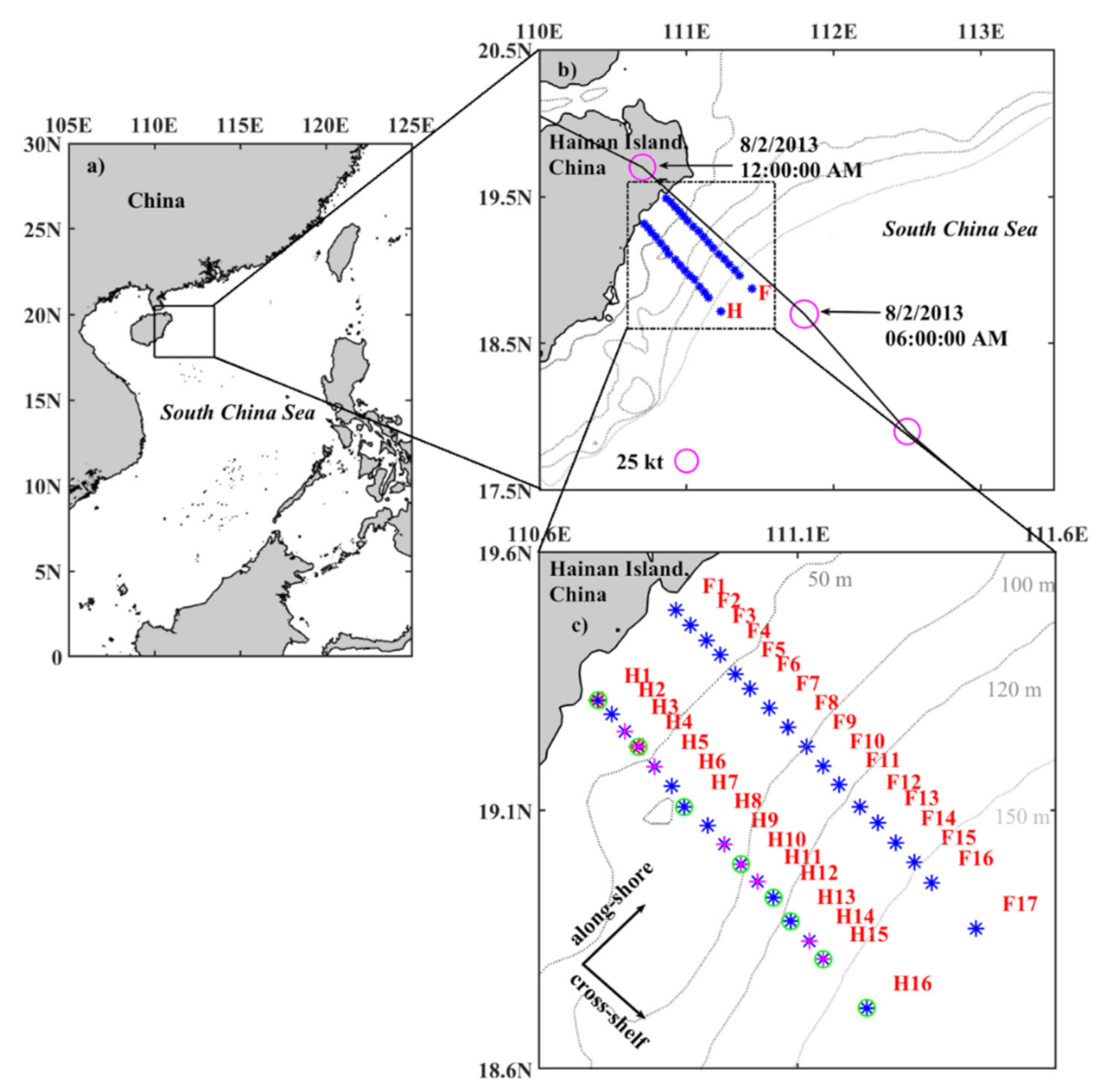
2.1. Study Area and Station Setting
2.2. Typhoon Chebi (2013)
2.3. Cruise Observation
2.4. Wind Data
2.5. Velocity Data Process
2.5.1. Tidal Currents
2.5.2. Along-Shore and Cross-Shelf Currents
2.6. Determination of Nutrients and Chlorophyll
2.7. Volume and Nutrient Fluxes
3. Results
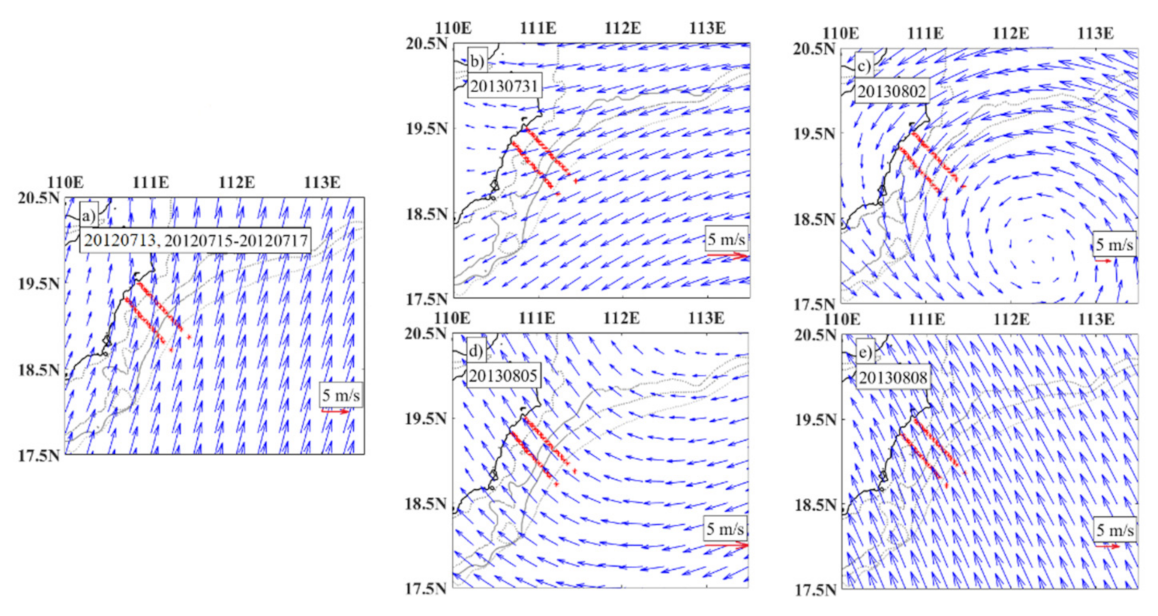
3.1. Wind Analysis
3.2. Changes in Current Field
3.2.1. Tidal Currents
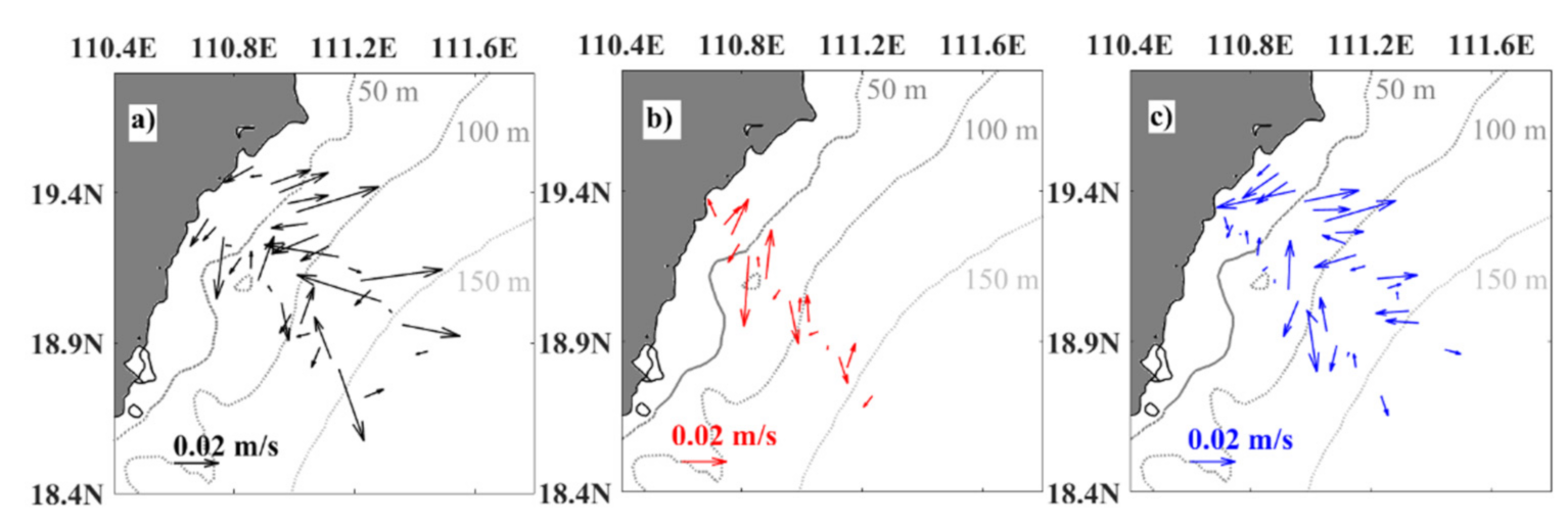
3.2.2. De-Tided Velocity Fields
3.2.3. Along-Shore and Cross-Shelf Currents
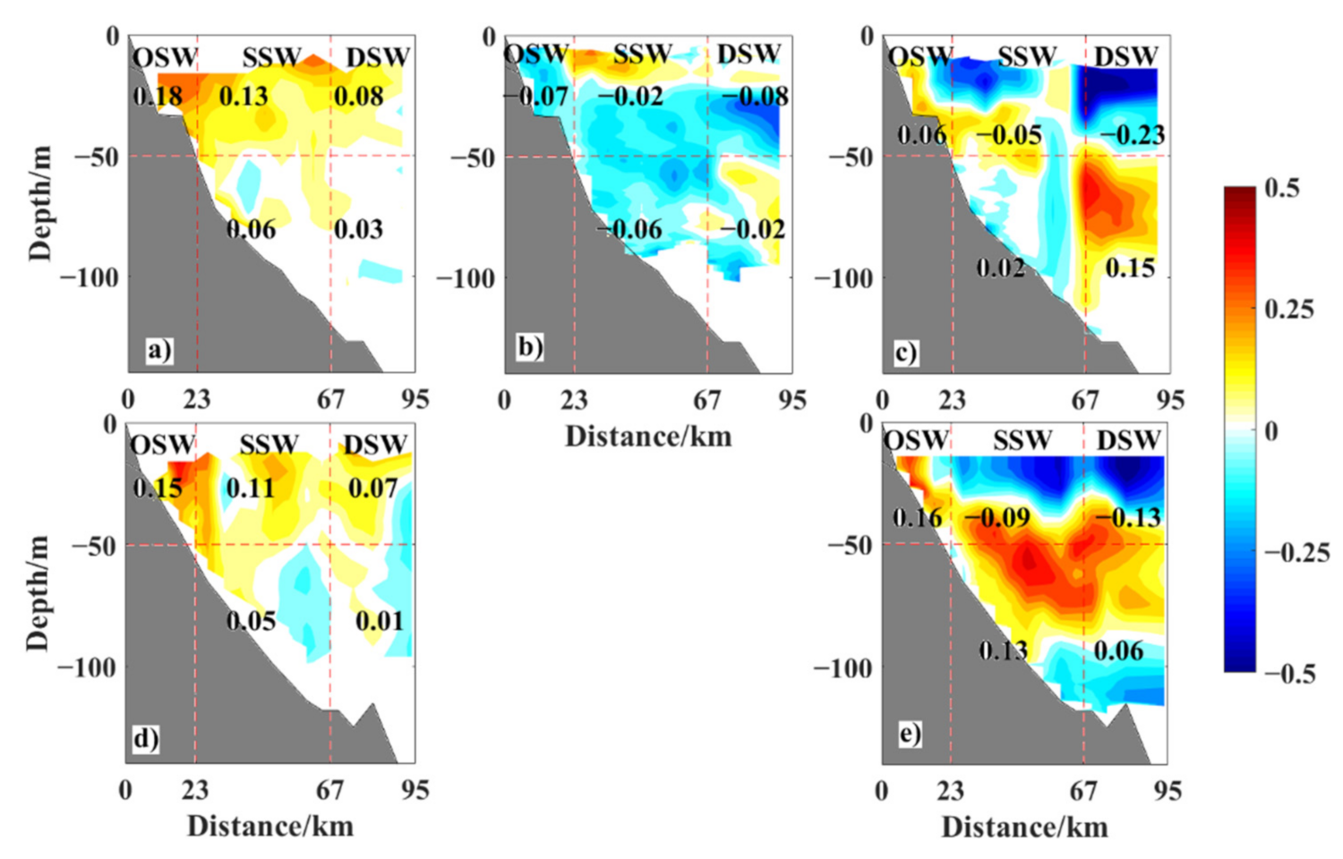
The Along-Shore Component
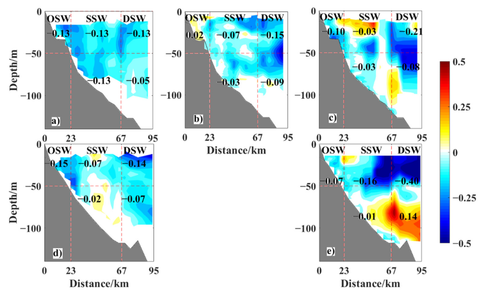
Cross-Shelf Component
3.3. Changes in Nutrient and Chl a
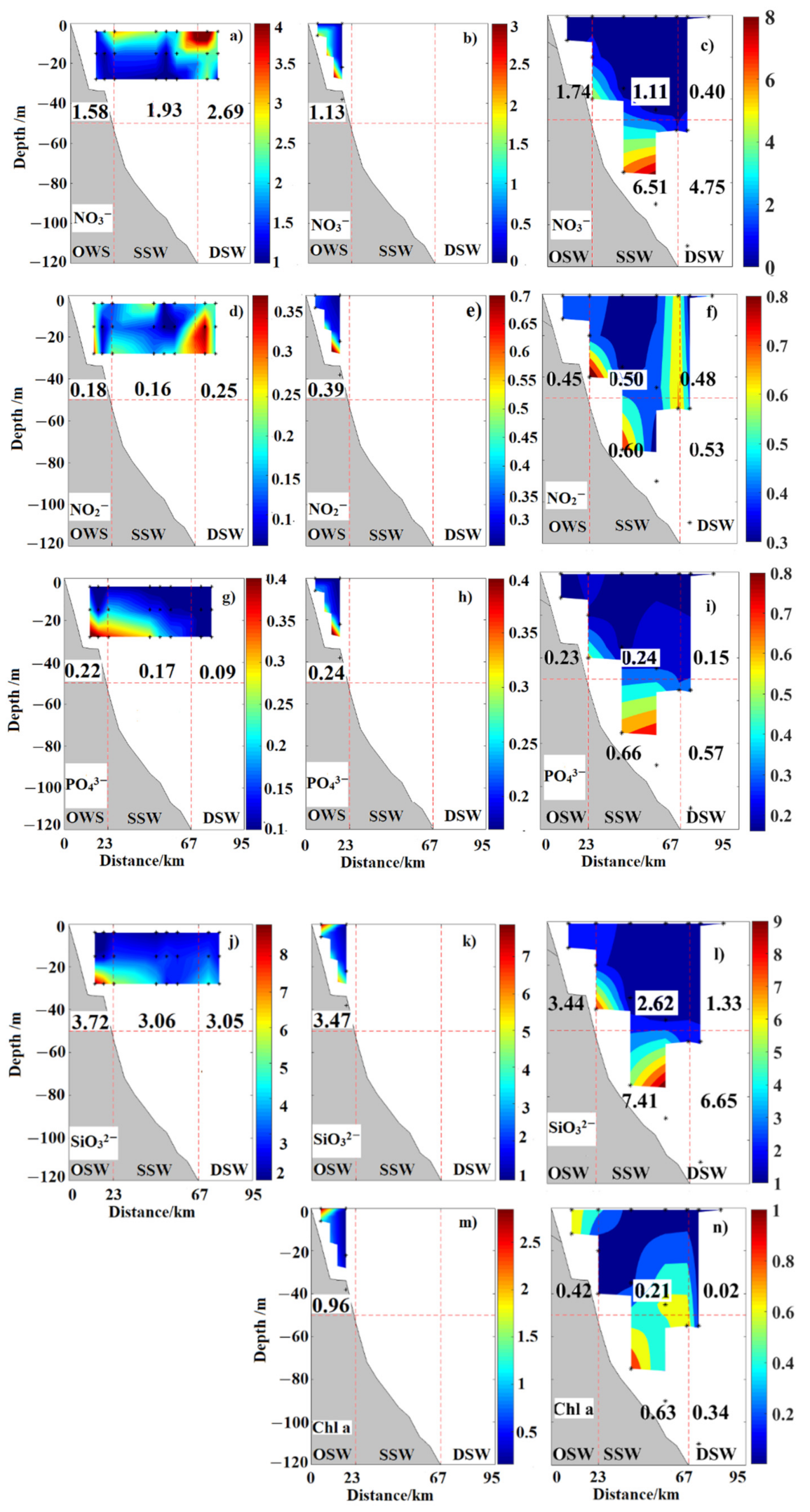
3.3.1. Distribution of Concentrations
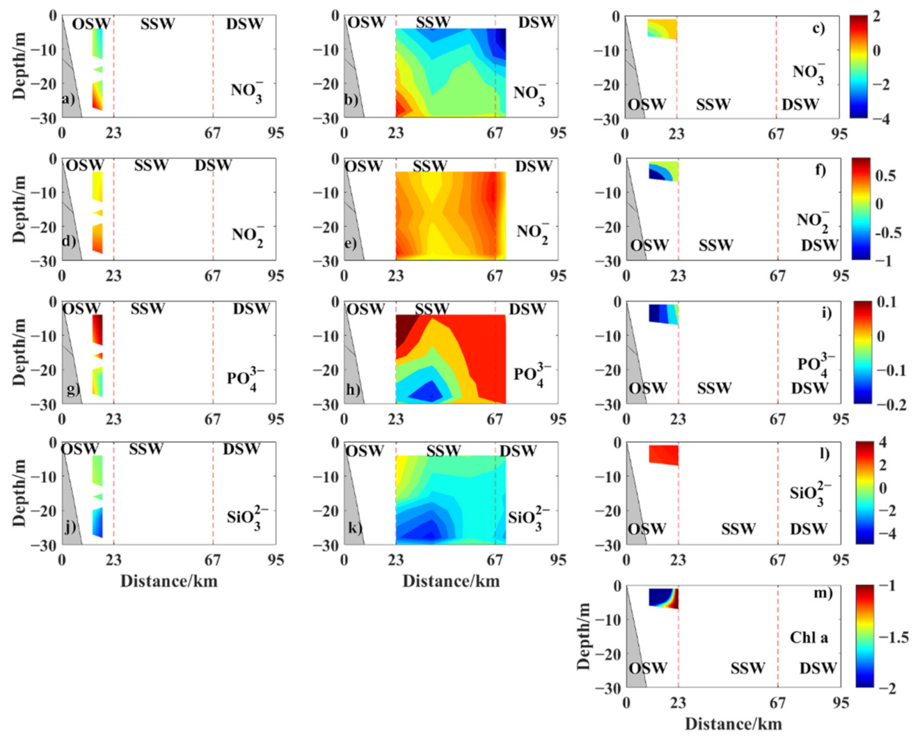
3.3.2. Variations of Concentrations
3.4. Volume and Nutrient Transports
3.4.1. Volume Transport
3.4.2. Nutrient Transports
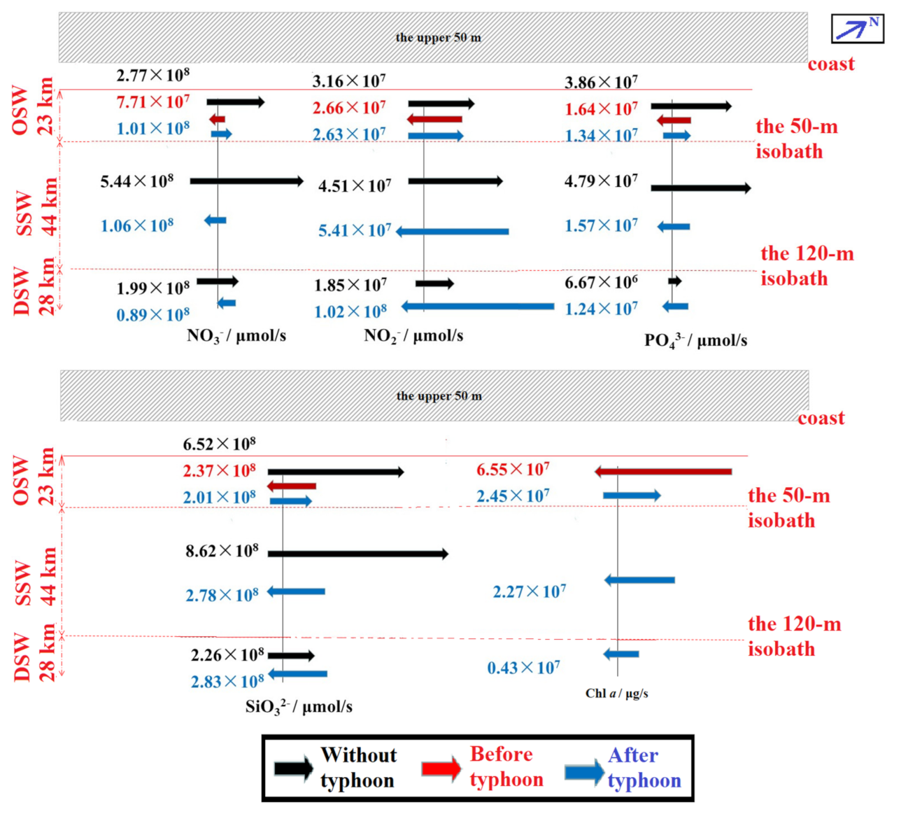
Along-Shore Fluxes
Cross-Shelf Fluxes
4. Discussion
4.1. Impacts of Tidal Current on Calculated Results
4.2. Volume Balance
4.3. Physical Mechanism
5. Conclusions
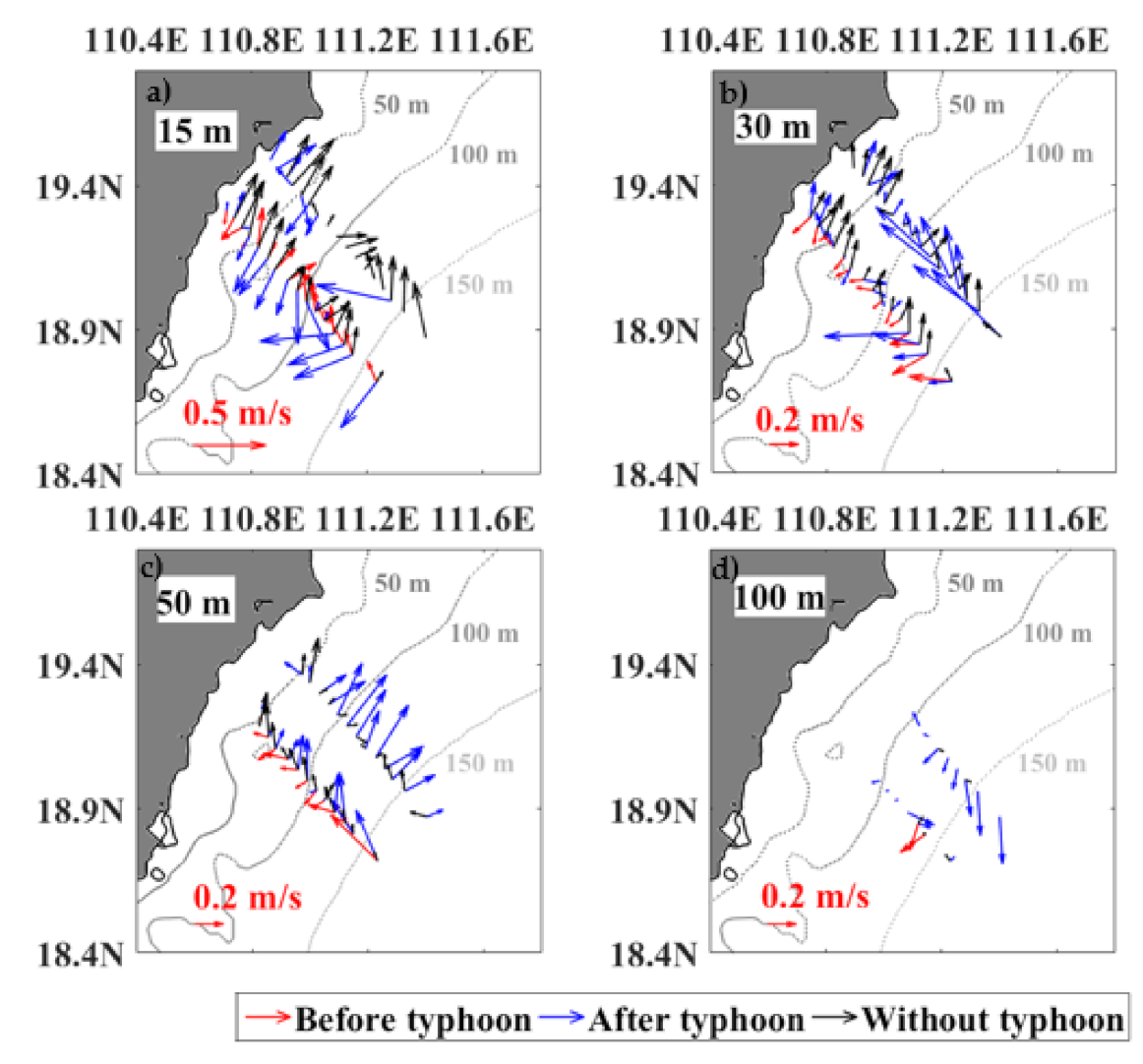
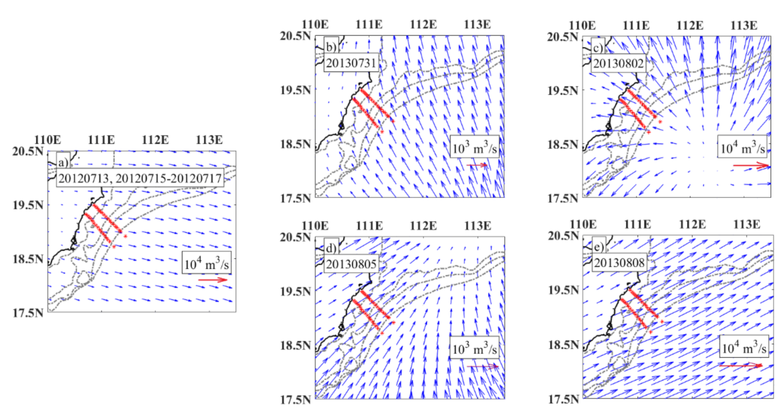
- In the case without the typhoon, the study area is controlled by the southwest monsoon. The current is mainly northeastward along the shore in the OSW and rotates counterclockwise to cross the shelf in the DSW and the deep layer below 50 m. The wind direction before the typhoon turns northeasterly. Meanwhile, the current direction changes into southwestward, starting from OSW to others, and velocity increases. In the case after the typhoon, the southerly winds prevail, and the current direction turns to be the same as that in the case without the typhoon. The vertical shear of horizontal velocity is greater than that in the case without the typhoon. There is water convergence near the 100 m isobath.
- In the case without the typhoon, the total along-shoreward volume transport mean is 0.64 × 10⁶ m3/s and the total cross-shelf transport mean is −0.28 × 10⁶ m3/s. In the case before the typhoon, however, the total along-shore transport is reversed southwestward and the average magnitude reduced to −0.34 × 10⁶ m3/s. The total cross-shelf transport mean is −0.27 × 10⁶ m3/s onshoreward, close to the value in the case without the typhoon. In the case after the typhoon, the total along-shore transport mean recovers to −0.09 × 10⁶ m3/s, while the total cross-shelf onshoreward transport mean increases by about 10% to −0.30 × 10⁶ m3/s.
- Compared with the along-shore nutrient fluxes in the case without the typhoon, in the case before the typhoon, all the fluxes in the OSW are reversed and smaller than those in the case without the typhoon, but Chl a is booming. In the case after the typhoon, the flux of NO3− in OSW has the same direction as, but decreases 64% in magnitude, while in the SSW and DSW, the fluxes are reversed and decrease 81% and 55% in magnitude, respectively. The fluxes of NO2−, PO34−, and SiO32− show similar behavior to that of NO3−, but have enhanced magnitudes, as high as 5.5, 1.9, and 1.3 times in DSW, respectively. However, the flux of Chl a in the OSW decreases to 37% of that in the case before the typhoon.
- Compared with the case without the typhoon, the typhoon passage, i.e., in the cases before and after the typhoon, greatly disturbs the distribution of nutrients. The averaged onshoreward transport fluxes in the OSW of NO3− decrease to 1/5 and 1/2, those of PO43− in the two cases decrease to 1/2, and those of SiO32− decrease to 1/3. On the contrary, the fluxes of NO2− in the two case changed little. Meanwhile, the onshoreward transport flux of Chl a decreases by 81% in the case after the typhoon in comparison to that in the case before the typhoon.
Author Contributions
Funding
Institutional Review Board Statement
Informed Consent Statement
Data Availability Statement
Conflicts of Interest
References
- Bauer, J.E.; Druffel, E.R.J.N. Ocean margins as a significant source of organic matter to the deep open ocean. Nature 1998, 392, 482. [Google Scholar] [CrossRef]
- Cai, W.J.; Dai, M.; Wang, Y. Air-sea exchange of carbon dioxide in ocean margins: A province-based synthesis. Geophys. Res. Lett. 2006, 33, 347–366. [Google Scholar] [CrossRef]
- Luo, X.F.; Wei, H. Progress on the study of continental shelf carbon cycle model. Adv. Mar. Sci. 2014, 32, 277–287. [Google Scholar]
- Su, J.L. Strengthening the investigation and study of offshore China. Adv. Earth Sci. 1996, 11, 7–9. [Google Scholar]
- Longhurst, A.; Sathyendranath, S.; Platt, T.; Caverhill, C. An estimate of global primary production in the ocean from satellite radiometer data. J. Plankton Res. 1995, 17, 1245–1271. [Google Scholar] [CrossRef]
- Wei-Jun, C. Comment on “Enhanced open ocean storage of CO2 from shelf sea pumping”. Science 2004, 306, 1477c. [Google Scholar]
- Brink, K.H. Cross-Shelf Exchange. Annu. Rev. Mar. Sci. 2016, 8, 59. [Google Scholar]
- Hong, B.; Wang, D.X. Dynamic diagnosis of winter upwind in the northern South China Sea. China Sci. Bull. 2006, 51, 9–14. [Google Scholar] [CrossRef]
- Fewings, M.; Lentz, S.J.; Fredericks, J. Observations of Cross-Shelf Flow Driven by Cross-Shelf Winds on the Inner Continental Shelf. J. Phys. Oceanogr. 2008, 38, 2358–2378. [Google Scholar] [CrossRef]
- Qiao, L.L.; Wang, Z.; Liu, S.D.; Li, G.X.; Liu, X.; Huang, L.L.; Xue, W.J.; Zhong, Y. From continental shelf seas to the western Pacific: The path and mechanism of cross-shelf suspended sediment transport in the Yellow Sea and East China Sea. Earth Sci. Front. 2017, 24, 134–140. [Google Scholar]
- Han, G. Three-dimensional seasonal-mean circulation and hydrography on the eastern Scotian Shelf. J. Geophys. Res. Ocean. 2003, 108, C53136. [Google Scholar] [CrossRef]
- Herman, F.; Rhodes, E.J.; Braun, J.; Heiniger, L. Uniform erosion rates and relief amplitude during glacial cycles in the Southern Alps of New Zealand, as revealed from OSL-thermochronology. Earth Planet. Sci. Lett. 2010, 297, 183–189. [Google Scholar] [CrossRef]
- Li, C. Cross-shelf passage of coastal water transport at the South Atlantic Bight observed with MODIS Ocean Color/SST. Geophys. Res. Lett. 2003, 30, 1257. [Google Scholar]
- Yuan, D.; Zhu, J.; Li, C.; Hu, D. Cross-shelf circulation in the Yellow and East China Seas indicated by MODIS satellite observations. J. Mar. Syst. 2008, 70, 134–149. [Google Scholar] [CrossRef]
- Dinniman, M.S.; Klinck, J.M. A model study of circulation and cross-shelf exchange on the west Antarctic Peninsula continental shelf. Deep-Sea Res. Part II 2004, 51, 2003–2022. [Google Scholar] [CrossRef]
- Dong, S.H.; Liu, S.M.; Ren, J.L.; Li, J.; Zhang, J. Preliminary estimates of cross shelf transport flux of nutrients in the East China Sea in spring. Mar. Environ. Sci. 2016, 35, 385–391. [Google Scholar]
- Wang, X.R.; Wang, Q.; Zhou, W.D.; Zhou, S.Q. Model diagnostic analysis of cross-shelf flow in the northern South China Sea. Chin. Sci. Bull. 2017, 62, 1059–1070. [Google Scholar]
- Liu, J.; Dai, J.; Xu, D.; Wang, J.; Yuan, Y. Seasonal and Interannual Variability in Coastal Circulations in the Northern South China Sea. Water 2018, 10, 520. [Google Scholar] [CrossRef]
- Deng, S.; Zhong, H.L.; Wang, M.W.; Yun, F.J. Upwelling along the coast of Qionghai and its relationship with fisheries. J. Oceanogr. Taiwan Strait 1995, 51–56. [Google Scholar]
- Jing, Z.; Qi, Y.; Du, Y.; Zhang, S.; Xie, L. Summer upwelling and thermal fronts in the northwestern South China Sea: Observational analysis of two mesoscale mapping surveys. J. Geophys. Res. Ocean. 2015, 120, 1993–2006. [Google Scholar] [CrossRef]
- Xie, L.L.; Guo, X.S.; Zhang, Y.W.; Kang, J.J. Reference velocity from bottom track in LADCP data processing. Ocean Technol. 2013, 32, 34. [Google Scholar]
- Chen, F.J.; Zeng, Z.; Meng, Y.F.; Zhu, Q.M.; Xie, L.L.; Zhang, S.W.; Chen, Q.X.; Chen, Q.X. Diel variation of nutrients and chlotophyll a concentration in the Qiongdong sea region during the summer of 2013. Haiyang Xuebao 2016, 38, 76–83. [Google Scholar]
- Jing, Z.; Qi, Y.; Du, Y. Upwelling in the continental shelf of northern South China Sea associated with 1997–1998 El Niño. J. Geophys. Res. Ocean. 2011, 116, C02033. [Google Scholar] [CrossRef]
- Xie, L.L.; He, C.F.; Li, M.M.; Tian, J.J.; Jing, Z.Y. Response of sea surface temperature to typhoon passages over the upwelling zone east of Hainan Island. Adv. Mar. Sci. 2017, 35, 8–19. [Google Scholar]
- Xie, L.; Zong, X.; Yi, X.; Li, M. The interannual variation and long-term trend of Qiongdong upwelling. Oceanol. Limnol. Sin. 2016, 47, 43–51. [Google Scholar]
- Zheng, M.L.; Li, M.M.; Xie, L.L.; Hong, Y.B.; He, Y.K.; Zong, X.L. Observational Analysis of Hydrographic Characteristics on the northwestern shelf of the South China Sea in winter 2012. Oceanol. Limnol. Sin. 2018, 49, 734–745. [Google Scholar]
- Su, J.; Wang, J.; Pohlmann, T.; Xu, D. The influence of meteorological variation on the upwelling system off eastern Hainan during summer 2007–2008. Ocean Dyn. 2011, 61, 717–730. [Google Scholar] [CrossRef]
- Tsai, Y.; Chern, C.S.; Wang, J. Numerical study of typhoon-induced ocean thermal content variations on the northern shelf of the South China Sea. Cont. Shelf Res. 2012, 42, 64–77. [Google Scholar] [CrossRef]
- Xie, L.; Pallàs-Sanz, E.; Zheng, Q.; Zhang, S.; Zong, X.; Yi, X.; Li, M. Diagnosis of 3D vertical circulation in the upwelling and frontal zones east of Hainan Island, China. J. Phys. Oceanogr. 2017, 47, 755–774. [Google Scholar] [CrossRef]
- Zhang, Y.; Tian, J. Enhanced turbulent mixing induced by strong wind on the South China Sea shelf. Ocean Dyn. 2014, 64, 781–796. [Google Scholar] [CrossRef]
- Zheng, Z.-W. Unusual warming in the coastal region of northern South China Sea and its impact on the sudden intensification of tropical cyclone Tembin (2012). Adv. Meteorol. 2014, 2014, 250752. [Google Scholar] [CrossRef]
- Guan, S.; Zhao, W.; Sun, L.; Zhou, C.; Liu, Z.; Hong, X.; Zhang, Y.; Tian, J.; Hou, Y. Tropical cyclone-induced sea surface cooling over the Yellow Sea and Bohai Sea in the 2019 Pacific typhoon season. J. Mar. Syst. 2021, 217, 103509. [Google Scholar] [CrossRef]
- Pan, A.; Guo, X.; Xu, J.; Jiang, H.; Xiaofang, W. Responses of Guangdong coastal upwelling to the summertime typhoons of 2006. Sci. China 2012, 55, 495–506. [Google Scholar] [CrossRef]
- Chang, Y.; Liao, H.T.; Lee, M.A.; Chan, J.W.; Lan, Y.C. Multisatellite observation on upwelling after the passage of Typhoon Hai-Tang in the southern East China Sea. Geophys. Res. Lett. 2008, 35, 154–175. [Google Scholar] [CrossRef]
- Shi, Y.X.; Xie, L.L.; Li, M.M.; Wan, L.; Zheng, M.L.; Shen, Y.F. Impacts of Typhoon Mujigea on Sea Surface Temperature and Chlorophyll-a Concentration in the Coastal Ocean of Western Guangdong. J. Guangdong Ocean Univ. 2017, 037, 49–58. [Google Scholar]
- Zhou, L.; Gao, S.; Yang, Y.; Zhao, Y.; Han, Z.; Li, G.; Jia, P.; Yin, Y. Typhoon events recorded in coastal lagoon deposits, southeastern Hainan Island. Acta Oceanol. Sin. 2017, 36, 37–45. [Google Scholar] [CrossRef]
- Li, J.; Zheng, Q.; Li, M.; Li, Q.; Xie, L.L. Spatiotemporal Distributions of Ocean Color Elements in Response to Tropical Cyclone: A Case Study of Typhoon Mangkhut (2018) Past Over the Northern South China Sea. Remote Sens. 2021, 13, 687. [Google Scholar]
- Yang, S.A.; He, L.F. Analysis of Atmosphere Circulation and Weather in August 2013. Meteorol. Mon. 2013, 39, 1521–1528. [Google Scholar]
- He, C.F. Analysis of the Impact and Mechanism of Tropical Cyclone on the Thermocline Features of Qiongdong Upwelling. Master’s Thesis, Guangdong Ocean University, Zhanjiang, China, 2016. [Google Scholar]
- Zeng, Z. Seasonal and Diel Variation of Nutrients and Chlorophyll a Concentration in the Qiongdong. Master’s Thesis, Guangdong Ocean University, Zhanjiang, China, 2015. [Google Scholar]
- Egbert, G.D.; Erofeeva, S.Y. Efficient Inverse Modeling of Barotropic Ocean Tides. J. Atmos. Ocean. Technol. 2002, 19, 183–204. [Google Scholar] [CrossRef]
- China National Standardization Management Committee. Specifications for Oceanographic Survey—Part 4: Survey of Chemical Parameters in Sea Water; China Standards Press: Beijing, China, 2007.
- China National Standardization Management Committee. Specifications for Oceanographic Survey—Part 6: Marine Biological Survey; China Standards Press: Beijing, China, 2007.
- Li, M.M.; Xie, L.L.; Zong, X.L.; Zhang, S.W.; Zhou, L.; Li, J.Y. The cruise observation of turbulent mixing in the upwelling region east of Hainan Island in the summer of 2012. Acta Oceanol. Sin. 2018, 37, 1–12. [Google Scholar] [CrossRef]
- Zhao, H.; Tang, D.L.; Wang, D. Phytoplankton blooms near the Pearl River Estuary induced by Typhoon Nuri. J. Geophys. Res. 2009, 114, C12027. [Google Scholar] [CrossRef]
- Wenping, G.; Jian, S.; Jianjun, J. Feedback between tidal hydrodynamics and morphological changes induced by natural process and human interventions in a wave-dominated tidal inlet: Xiaohai, Hainan, China. Acta Oceanol. Sin. 2009, 96–116. [Google Scholar]
- Wang, F.Y.; Qiu, L.G.; Liang, X.L.; Mo, W.Y.; Liang, N.A.; Wang, Y.Z. Response of human activities on tidal hydrodynamics of Hainan Qinglan tidal inlet system based on Delft 3D model. Quat. Sci. 2018, 38, 496–504. [Google Scholar]
- Zheng, M.L. Seasonal Variability of 3D Volume and Nutrient Transports in the Northwestern South China Sea. Master’s Thesis, Guangdong Ocean University, Zhanjiang, China, 2019. [Google Scholar]


| NO3− (μmol/s) | NO2− (μmol/s) | PO43− (μmol/s) | SiO32− (μmol/s) | Chl a (μg/s) | |
|---|---|---|---|---|---|
| Without the typhoon | 367.31 | 41.10 | 51.73 | 866.13 | N/A |
| Before the typhoon | −104.52 | −39.83 | −24.11 | −292.93 | −61.03 |
| After the typhoon | 134.07 | 34.21 | 17.96 | 267.01 | 11.30 |
| NO3− (μmol/s) | NO2− (μmol/s) | PO43− (μmol/s) | SiO32− (μmol/s) | Chl a (μg/s) | |
|---|---|---|---|---|---|
| Without the typhoon | −341.18 | −27.92 | −39.70 | −632.74 | N/A |
| Before the typhoon | −73.16 | −36.77 | −21.28 | −228.25 | −20.54 |
| After the typhoon | −153.33 | −22.58 | −11.33 | −239.61 | −3.89 |
| Section H (m/s) | Section F (m/s) | |
|---|---|---|
| Without the typhoon | 0.09/0.09 | 0.07/0.07 |
| Before the typhoon | −0.05/−0.05 | N/A |
| After the typhoon | 0.01/0.01 | 0.02/0.01 |
| Section H (m/s) | Section F (m/s) | |
|---|---|---|
| Without the typhoon | −0.11/−0.11 | −0.07/−0.07 |
| Before the typhoon | −0.06/−0.06 | N/A |
| After the typhoon | −0.05/−0.05 | −0.05/−0.07 |
Publisher’s Note: MDPI stays neutral with regard to jurisdictional claims in published maps and institutional affiliations. |
© 2021 by the authors. Licensee MDPI, Basel, Switzerland. This article is an open access article distributed under the terms and conditions of the Creative Commons Attribution (CC BY) license (http://creativecommons.org/licenses/by/4.0/).
Share and Cite
Zheng, M.; Xie, L.; Zheng, Q.; Li, M.; Chen, F.; Li, J. Volume and Nutrient Transports Disturbed by the Typhoon Chebi (2013) in the Upwelling Zone East of Hainan Island, China. J. Mar. Sci. Eng. 2021, 9, 324. https://doi.org/10.3390/jmse9030324
Zheng M, Xie L, Zheng Q, Li M, Chen F, Li J. Volume and Nutrient Transports Disturbed by the Typhoon Chebi (2013) in the Upwelling Zone East of Hainan Island, China. Journal of Marine Science and Engineering. 2021; 9(3):324. https://doi.org/10.3390/jmse9030324
Chicago/Turabian StyleZheng, Manli, Lingling Xie, Quanan Zheng, Mingming Li, Fajin Chen, and Junyi Li. 2021. "Volume and Nutrient Transports Disturbed by the Typhoon Chebi (2013) in the Upwelling Zone East of Hainan Island, China" Journal of Marine Science and Engineering 9, no. 3: 324. https://doi.org/10.3390/jmse9030324
APA StyleZheng, M., Xie, L., Zheng, Q., Li, M., Chen, F., & Li, J. (2021). Volume and Nutrient Transports Disturbed by the Typhoon Chebi (2013) in the Upwelling Zone East of Hainan Island, China. Journal of Marine Science and Engineering, 9(3), 324. https://doi.org/10.3390/jmse9030324