Numerical Study of Hydrodynamics of Heavily Loaded Hard-Chine Hulls in Calm Water

Abstract

Hard-chine boats are usually intended for high-speed regimes where they operate in the planing mode. These boats are often designed to be relatively light, but there are special applications that may occasionally require fast boats to be heavily loaded. In this study, steady-state hydrodynamic performance of nominal-weight and overloaded hard-chine hulls in calm water is investigated with computational fluid dynamics solver program STAR-CCM+. The resistance and attitude values of a constant-deadrise reference hull and its modifications with more pronounced bows of concave and convex shapes are obtained from numerical simulations. On average, 40% heavier hulls showed about 30% larger drag over the speed range from the displacement to planing modes. Among the studied configurations, the hull with a concave bow is found to have 5–12% lower resistance than the other hulls in the semi-displacement regime and heavy loadings and 2–10% lower drag in the displacement regime and nominal loading, while this hull is also capable of achieving fast planing speeds at the nominal weight with typical available thrust. The near-hull wave patterns and hull pressure distributions for selected conditions are presented and discussed as well.

1. Introduction

Fast planing boats usually employ hard-chine hulls to ease water separation at high speeds from their hulls, which leads to drag reduction. Relatively small areas on hull surfaces need to stay in contact with water to provide a hydrodynamic lift sufficient for carrying the boat weight. To achieve high speeds, power requirements for fast boats with hard chines are still much greater than those of displacement boats moving at low speeds. Therefore, to keep planing boats reasonably economical, they are usually designed to be relatively light. The weight $W$ of a fast boat can be normalized by the hull beam $B$, forming a beam-based loading coefficient,

$$C_B=\frac{W}{\gamma B^3},$$

(1)

where $\gamma$ is the specific weight of water. This coefficient is usually limited by 0.9 for planing hulls, while most fast boats are much lighter. However, hard-chine hulls operating with $C_B>1$ also exist.

When describing different speed regimes of boats and ships, a non-dimensional Froude number is commonly used,

$$F{r}_c=\frac{u}{\sqrt{gc}}$$

(2)

where $u$ is the speed, $g$ is the gravity constant, and $c$ is the characteristic length. Various length parameters are utilized for Froude number in ship hydrodynamics, including the hull length, $L$, waterline length, hull beam, and a cubic root of the volumetric displacement, $\sqrt[3]{V}$. The planing regime usually corresponds to the Foude length number $F{r}_L=u/\sqrt{gL}>1–1.2$ or the volumetric Froude number $F{r}_V=u/\sqrt{g{V}^{1/3}}>3–4$ [1,2,3].

Although not very common, there are applications demanding heavily loaded fast marine transports. For example, during rescue missions, a boat may have to carry a higher payload than it was designed for. There are also a variety of special operations when boats with relatively small footprints need to transport heavy cargo at high speeds. To assess the hydrodynamic performance of boats in such conditions, namely to estimate achievable speeds (which will be of course lower than at normal loading), thrust requirements and other parameters, one needs to know the hull drag and attitude behavior in a broad range of speeds and loadings. However, the literature on the hydrodynamics of hard-chine planing hulls is essentially limited to conditions with the beam loading coefficient around 0.9 at moderate Froude numbers.

Among the approaches used for predicting hydrodynamics of usual planing hulls, empirical correlations, such as the Savitsky’s method [2], are still very popular, but due to a small number of involved parameters and a broad range of possible conditions, they can be applied only for initial approximate estimations. A review of empirical methods and illustrations of hull forms intended for different high-speed regimes, including relatively heavy hard-chine hulls, is given by Almeter [4]. A variety of potential-flow modeling methods that can account for specific hull geometries have been developed in the past [5,6,7], but they ignore viscous effects and are often applicable only at sufficiently high Froude numbers. With the growth of available computational power, numerical methods accounting for viscosity and flow non-linearities are becoming widely used for ship hydrodynamics studies, including fast boats [8,9,10,11]. These computational fluid dynamics (CFD) tools can, therefore, be applied for modeling heavily loaded hard-chine hulls in the entire speed range. In the present study, one such CFD program (STAR-CCM+) is utilized. The authors of this paper have previously conducted a validation study of planing hulls employing a similar CFD approach [12].

The present paper has several objectives. One is to show validation of CFD for a relatively heavy constant-deadrise planning hull with $C_B\approx 0.9$, for which experimental data are available. Secondly, an overloaded (by 40%) condition of this and other hull forms is simulated to expand the knowledge base of heavy hard-chine hulls in the range of speeds from the displacement to planing states. In addition, more practical hulls with extended bow portions that have convex and concave shapes are also generated, and their hydrodynamic characteristics are quantified as well. Most simulations are conducted here with one common location of the longitudinal center of gravity (LCG), at 45% of the hull length from the transom. Several simulations of overloaded hulls in the transitional regime are also carried out with LCG = 40% to compare the performance of concave and convex bows.

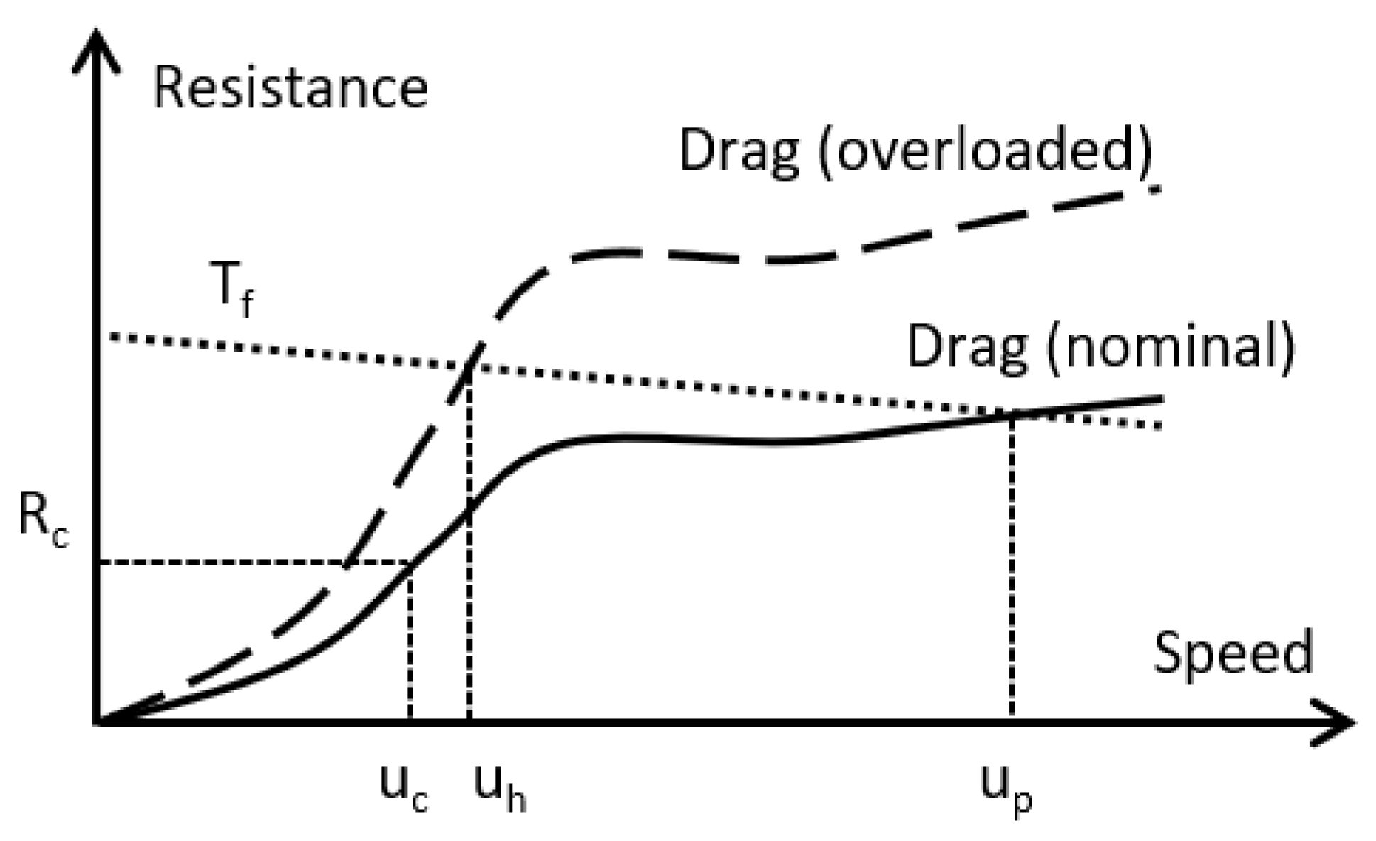
Figure 1 graphically illustrates some practical motivations that guided the present study. One of the intentions is to determine a suitable hull form that would be economical at the nominal weight in the semi-displacement mode at cruise speed $u_c$ (Figure 1), i.e., it will have reasonably low resistance $R_c$ within $F{r}_L ~ 0.5–0.8$ or $F{r}_V ~ 0.7–1.7$. At the same time, this hull at the nominal weight should be able to reach a planing speed $u_p$ ($F{r}_L ~ 1.2, F{r}_V ~ 3.0$) with full thrust typical for planing hulls $T_f$. The specific characteristic of most interest in the present study is the boat’s ability to archive the highest speed $u_h$ (among the considered hulls) under the same available thrust in the overloaded condition. It should be noted that only steady-state forward motion in calm water was analyzed here. Other important hydrodynamic characteristics, such as seaworthiness and maneuvering, are beyond the scope of this paper. Studies on those topics with applications to semi-displacement and planning hulls can be found in [3,9,13].

The novelty and contributions of this work include results for hydrodynamics of heavily loaded hard-chine hulls that are not available in the literature, so the practitioners can use these data to quickly access the performance of overloaded planing hulls. A systematic comparison of hydrodynamic performance is presented for various bow shapes, so a specific bow form can be used as a starting point in designing a heavy hull for intended speed regimes. Contributions are also made to the computational methodology for fast boat hydrodynamics. A three degree of freedom unsteady approach used to achieve steady states has been described. Comparisons are presented for different turbulence models and computational times at various speeds and loading conditions.

The rest of the paper is organized as follows. In Section 2, a description is given for the hull geometries, as well as speed and loading conditions. Section 3 elaborates on computational aspects, including the numerical domain, grid specifics, governing equations and modeling of the hull dynamics in transient regimes. The verification and validation studies, involving a comparison with experimental data, are shown in Section 4. The results of extensive parametric studies performed in this work for various hull geometries, loadings and speeds are presented and discussed in Section 5, which is followed by the conclusions.

2. Hull Geometries and Studied Conditions

The hull geometries studied in this work are relatively basic (Figure 2 and Figure 3). Three different bow shapes were analyzed: constant-deadrise, concave, and convex hull shapes. Only two locations of the center of gravity were investigated, 40% and 45% of the hull total length from the transom. Two loading conditions were looked at, $C_B$ = 0.912 and $C_B$ = 1.276. The lower value corresponds to a relatively heavy planing hull, but within a common range of loadings. The higher value, obtained by increasing the hull weight by 40%, imitates an overloaded state or a special compact fast boat intended for heavy cargo.

The constant-deadrise basis hull with the selected loading $C_B$ = 0.912 comes from the family of hulls experimentally studied by Fridsma [13]. Its length-to-beam ratio is 5, and the deadrise angle is 10°. The experimental hull was 1.143 m long, and the length of the non-prismatic bow section was 0.229 m or 20% of the hull length (Figure 2).

Two modified hull shapes were numerically generated in this study with the purpose to improve hydrodynamic characteristics in the semi-displacement regime. They have convex and concave bow shapes, shown in Figure 3, while the curved bow portion was extended to 40% of the fore part of the hull. (Initially, hulls with curved bows of 20% length overall (LOA) were also tried in this work, but due to the bow exit out of water with increasing speeds, their performance difference from the original hull was limited to a narrow range of relatively low speeds.) The aft body of hulls with curved bows was kept prismatic and identical to the constant-deadrise hull.

In most simulations, the longitudinal center of gravity (LCG) was placed at 45% of the overall length, as measured from the stern (Figure 2), although a limited set of simulations was also conducted with LCG at 40%. The vertical position of the center of gravity was 47% of the hull height or 5.9% of LOA, counted up from the keel line on the prismatic hull portion.

The lines plan for hulls of the three different bow shapes are shown in Figure 3. The geometry of hulls with curved bows was parameterized with three equally spaced transverse splines in the bow region such that the convexity and concavity were arced by the same amount, but in different directions. The maximum arc for the three splines, going from bow to stern were 4.44%, 1.11%, and 0.56% of the hull beam, respectively.

An additional hull feature in experiments of Fridsma [13] was a very small strip positioned at the chine along the prismatic portion of the hulls. This thin strip was used to prevent wetting of the hull side walls at sufficiently high speeds on the model scale that would likely not be seen if the hull was operating in full-scale conditions. This thin strip was modeled in all simulations in the same manner as described by Wheeler et al. [12].

In the parametric simulations of this study for LCG = 45% conditions, the speed range was selected between 0.25 and 1.50 of length-based Froude numbers defined by Equation (2). Given the limitation of accessible computational resources, only the model-scale hulls were investigated, corresponding to experimental dimensions [13]. The range of length-based Reynolds numbers in the chosen speed range was between 5.4 × 10⁵ and 3.2 × 10⁶. For the LCG = 40% conditions, the parametric calculations were carried out only in the transitional speed regime at heavy loading and in a wider speed range at nominal loading for validation purposes.

3. Computational Approach

The present study consisted of a number of simulations, and in order to ensure similar numerical accuracy for all cases, a mesh template was employed such that all geometries and simulated conditions had as similar computational grids as possible. For the reference length in the meshing procedure, a base size of L/25 (L being the hull length) or 4.6 cm in dimensional units was selected, and all meshing parameters were based on this length.

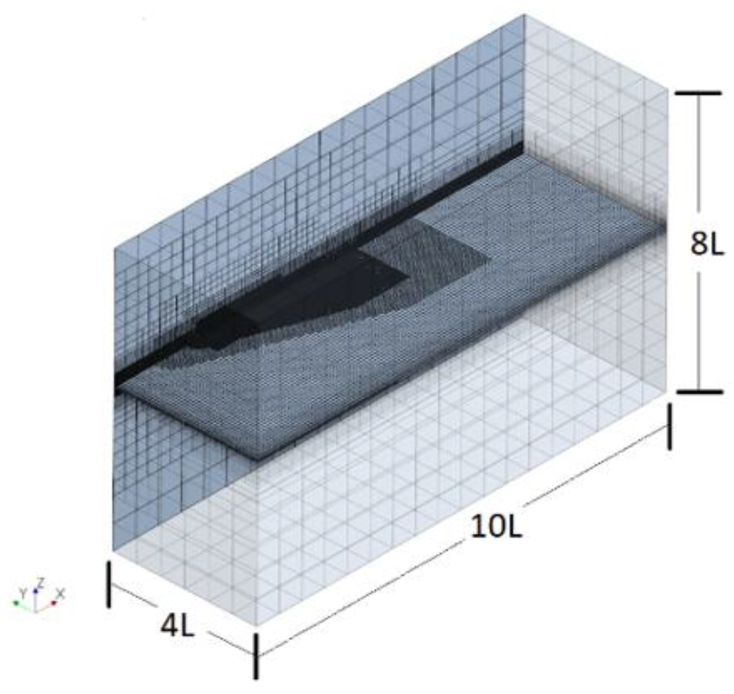
There were two primary fluid domains used in the computations. The first region was a larger, background region, which consisted of octree-formed hexahedral cells (Figure 4). Mesh refinements were implemented in the area near the free surface and in the areas in the wake region of the hull. The domain used an anisotropic refinement in the Z (vertical) direction of 25% of base size throughout those zones. In addition, isotropically refined cells of 25% base size were used in the areas near the hull and the area of the expected near-field wave generation. Only half of the fluid region on the port side from the hull centerplane was considered. The dimensions of the fluid domain were based on the hull length and were selected as 10 L × 4 L × 8 L (Figure 4).

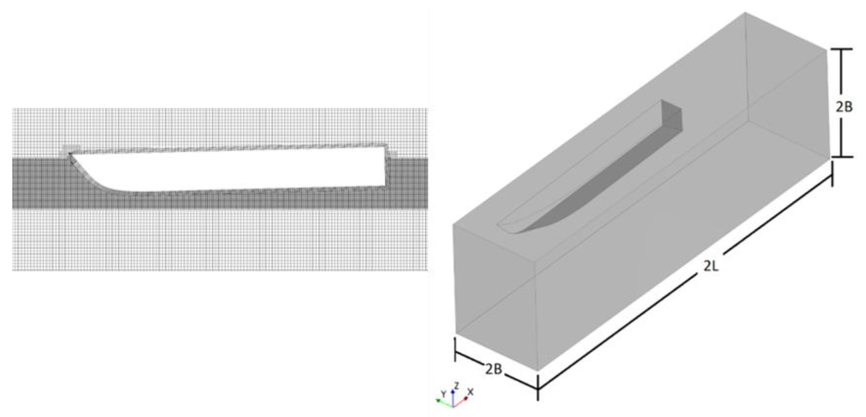
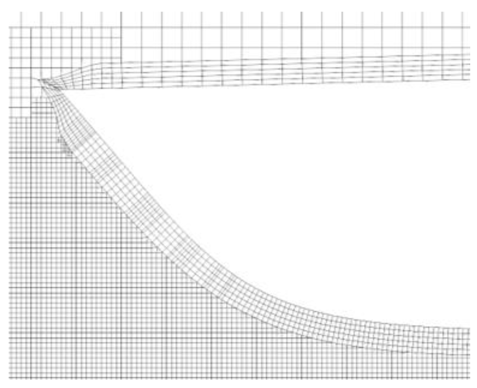
The second (overset) region encompassed the vessel and used an octree formed trimmed cell mesh with five prism layers along the surface of the hull. The size of this region was chosen by using both length and beam, with the dimensions being 2L × 2B × 2B as shown in Figure 5. Special care was used in the prism layer generation process to ensure the wall Y+ was within the acceptable range. All simulations had surface averaged Y+ values in the range between 30 and 100; therefore, empirical wall functions were used to approximate the flow turbulence. The near wall cell size of the hull was set to 6.25% of the base size. In addition, the prism layer thickness and number of layers were carefully chosen such that the cell size in the outermost layer of the prism layer mesh matched the cell size in the near-wall trimmed mesh (Figure 6). This matching produced a more uniform mesh, which, together with moderate Reynolds numbers used in this study, helped eliminate numerical ventilation. Numerical ventilation is known to be a challenging problem arising in ship hull simulations that rely on the volume-of-fluid (VOF) approach. To address this problem, a common recommendation is to employ very fine numerical grids and very small time steps which, however, may be very computationally prohibitive. Alternative methods include the artificial suppression of the ventilation, such as the phase replacement, corrections to the interface capturing scheme and more gradual transitions between the prism mesh and the volume mesh [12,14,15].

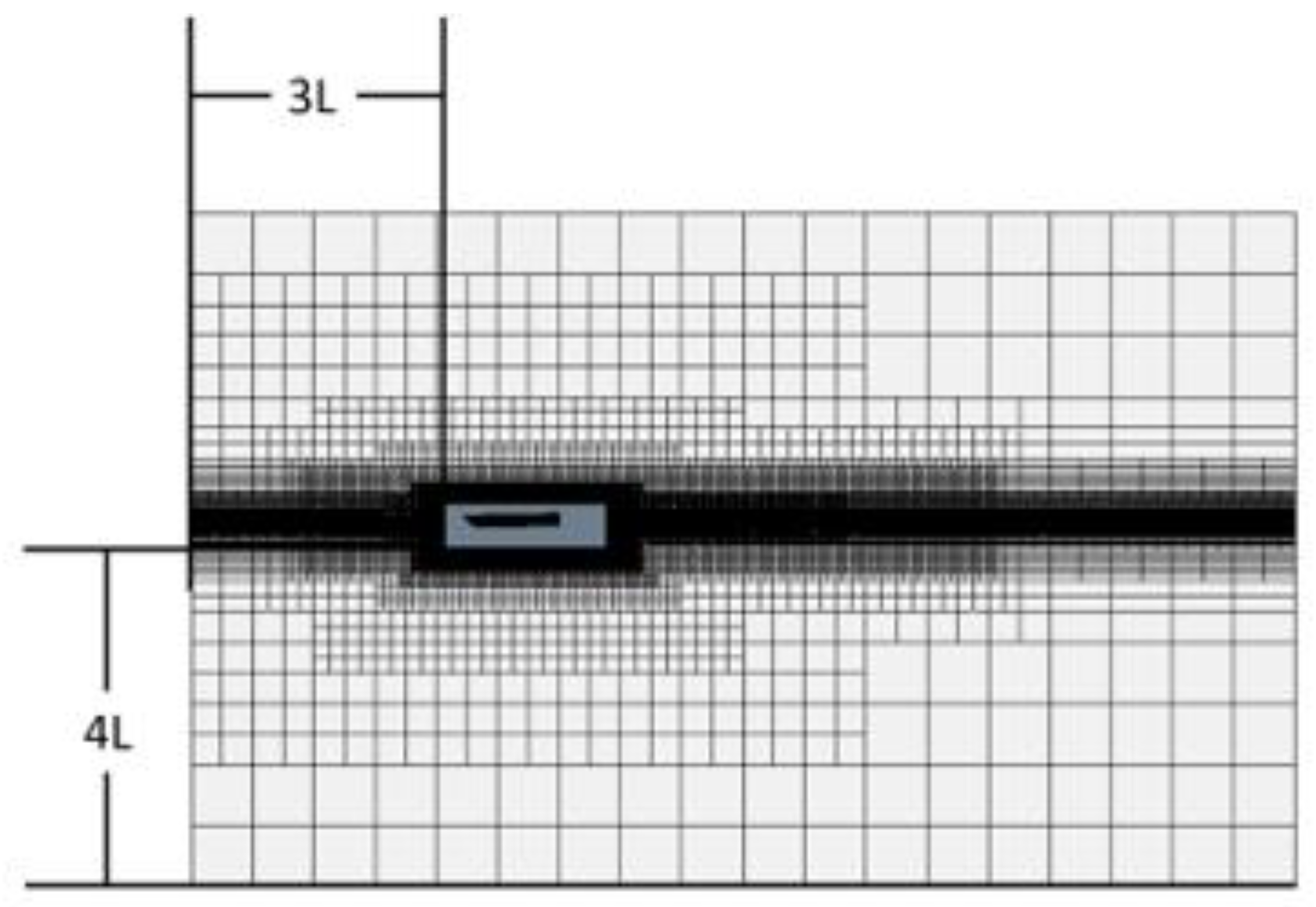
The two regions (background and overset) were then interfaced together using overset interfaces with the linear interpolation scheme. The overset region was placed 3 L behind the inlet and 4 L above the domain bottom as shown in Figure 7. A three-degree-of-freedom (3-DOF) unsteady approach was used to find the steady-state resistance, trim, and sinkage of the vessel. The three degrees of freedom of the vessel were surge, pitch, and heave, or in other words, translation in X and Z directions and rotation about the Y axis passing through of the hull’s center of gravity. The background and overset region moved in surge, but only the overset region pitched and heaved. The vessel was initially at rest in a calculated hydrostatic equilibrium state. The vessel was then artificially accelerated from rest using an assumed constant acceleration (1 m/s²) via a point force attached to the hull’s center of mass. The force applied was equal to the drag of the vessel plus the mass of the hull multiplied by the assumed acceleration. This force was exerted until the vessel reached the speed of interest, at which the applied point force became simply equal to the vessel’s instantaneous drag force. The reason for using this approach in lieu of the more traditional 2-DOF approach with the constant incoming flow was due to significant hull motions when the simulation was started with at-rest initial conditions. It was found that some hulls would initially exhibit severe motions due to the abrupt (unrealistic) start of the flow if the starting conditions were far from the steady-state conditions at speed. These oscillating motions would then require a long time to dampen out in the simulation. Since the final steady-state condition was not known beforehand, but it was the main objective in these simulations, the 3-DOF method was used. The hydrostatic resting position of the hull can be calculated quickly and accelerating it from rest provides a natural and more realistic evolution of the vessel’s sinkage and trim. This approach proved to have a much faster turnaround for this study than the traditional 2-DOF method [10,16].

The STAR-CCM+ segregated flow solver employing the SIMPLE (Semi-Implicit Method for Pressure Linked Equations) algorithm with second-order convection terms was utilized in this study. The first-order implicit stepping in time was conducted until the time-averaged flow characteristics were no longer evolving. The Eulerian multi-phase method with constant-density air and water, properties of which were consistent with experimental conditions [13]. The high-resolution interface capturing the (HRIC) approach within the volume-of-fluid (VOF) method was employed for resolving the air–water interface. The main fluid mechanics equations used by the solver include the continuity, momentum and VOF equations,

$$\nabla \cdot \overline{v}=0,$$

(3)

$$\frac{\partial }{\partial t}\left(\rho \overline{v}\right)+\nabla \cdot \left(\rho \overline{v}\otimes \overline{v}\right)=-\nabla \cdot \left(\overline{p}I\right)+\nabla \cdot \left(T+T_t\right)+f_b,$$

(4)

$$\frac{\partial c}{\partial t}+\nabla \cdot \left(c\overline{v}\right)=0,$$

(5)

where $v$ is the flow velocity vector, $\rho$ is the density of the mixture, $p$ is the pressure, $I$ is the identity tensor, $T$ is the viscous stress tensor,$T_t$ is the Reynolds stress tensor, $f_b$ is the gravitational body force, and $c$ stands for the volume fraction taken by air. Then, the effective fluid density ρ and viscosity µ are found as $\rho ={\rho }_{air}c+{\rho }_{water}\left(1-c\right)$ and $\mu ={\mu }_{air}c+{\mu }_{water}\left(1-c\right)$. The overbar in Equations (3)–(5) correspond to mean flow properties. The Boussinesq hypothesis is used to model the Reynolds stresses,

$$-\rho \overline{{u^{\prime }}_i{u^{\prime }}_j}={\mu }_t\left(\frac{\partial u_i}{\partial x_j}+\frac{\partial u_j}{\partial x_i}\right)-\frac{2}{3}\rho k{\delta }_{ij},$$

(6)

where $k$ is the turbulent kinetic energy and ${\mu }_t$ is the turbulent eddy viscosity.

The Reynolds averaged Navier–Stokes (RANS) approach with the realizable $k-\epsilon$ Two-Layer All-Y+ turbulence model available in Star-CCM+ was utilized [17,18]. The realizable $k-\epsilon$ model is the most common method in CFD ship hydrodynamics [19]. Other turbulence models were also tried in several conditions (as described in the next section), but they produced results very similar to the Realizable $k-\epsilon$ model. The governing equations of this model for the turbulent kinetic energy $k$ and the turbulent dissipation rate $\epsilon$, as well as the expression for the turbulent viscosity ${\mu }_t$, are given as follows,

$$\frac{\partial \left(\rho k\right)}{\partial t}+\frac{\partial \left(\rho k{\overline{u}}_j\right)}{\partial x_j}=\frac{\partial }{\partial x_j}\left[\left(\mu +\frac{{\mu }_t}{{\sigma }_k}\right)\frac{\partial k}{\partial x_j}\right]+G_k-\rho \epsilon ,$$

(7)

$$\frac{\partial \left(\rho \epsilon \right)}{\partial t}+\frac{\partial \left(\rho \epsilon {\overline{u}}_j\right)}{\partial x_j}=\frac{\partial }{\partial x_j}\left[\left(\mu +\frac{{\mu }_t}{{\sigma }_{\epsilon }}\right)\frac{\partial \epsilon }{\partial x_j}\right]+\rho C_{\epsilon 1}S\epsilon -\rho C_{\epsilon 2}\frac{{\epsilon }^2}{k+\sqrt{\nu \epsilon }},$$

(8)

$${\mu }_t=\rho C_{\mu }\frac{k^2}{\epsilon },$$

(9)

where $G_k$ is responsible for turbulent production, $S$ is the magnitude of the mean strain rate tensor, $\nu$ is the kinematic viscosity, ${\sigma }_k$, ${\sigma }_{\epsilon }$, $C_{\epsilon 1}$, $C_{\epsilon 2}$ are the model parameters [20], and $C_{\mu }$ depends on both the mean flow and turbulence properties [21].

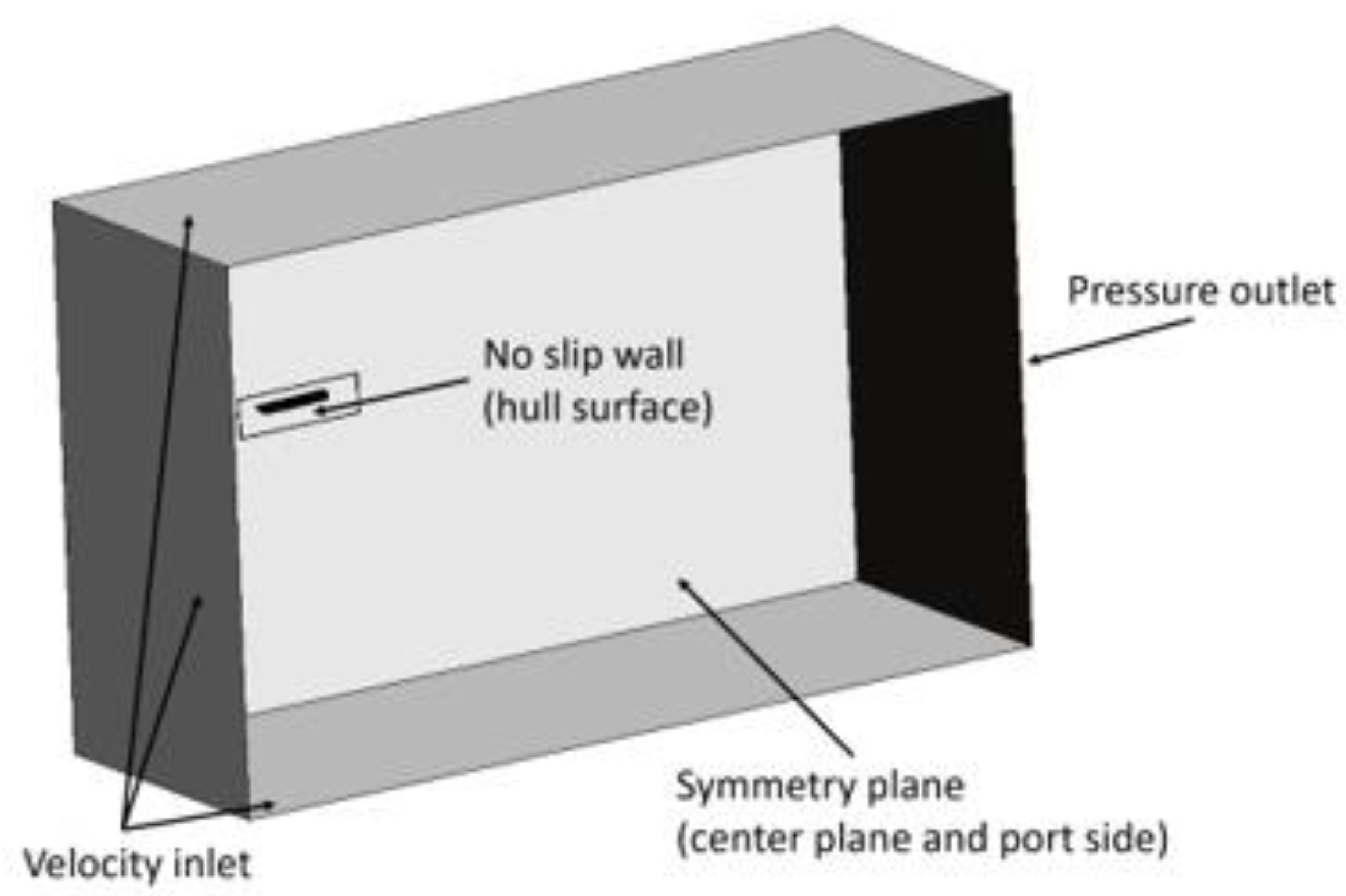
Following ITTC recommendations on CFD simulations [22], near and at steady-state regimes the time step was selected as L/(250 U), where U is the hull velocity. Five inner iterations were performed at each time step during the simulations. The initial conditions included the undisturbed fluid at rest. The boundary conditions were specified as shown in Figure 8. The downstream boundary is the pressure outlet with the hydrostatic pressure gradient. The symmetry plane passed through the hull centerplane. The no-slip condition was imposed on the hull surface. Other sides of the domain were treated as the velocity inlets with zero flow condition since the entire mesh moves forward at a rate equivalent to the hull speed. The wave forcing zones of 80% of hull length were applied at the port-side boundary and the upstream and downstream boundaries. The wave forcing method involves activation of momentum sources near domain boundaries that adapt the solution to specified boundary conditions [20]. This way, one can minimize undesirable numerical wave reflections and thus use more compact (economical) numerical domains.

4. Verification and Validation

Solution verification study was conducted at two conditions with $C_B$ = 0.912, for which experimental data [13] are also available. Condition (1) involves LCG = 45% and Fr_V = 1.67 (transitional regime), whereas condition (2) corresponds to LCG = 40% and Fr_V = 2.68 (close to planing regime). To perform the verification, solutions were obtained on three mesh levels with different characteristic cell size. The base size was changed by factors of $\sqrt{2}$ for three mesh levels. The corresponding time step was also changed by a factor of $\sqrt{2}$ as well to keep the Courant number the same between grids. As an indicator of the solution convergence, the drag coefficient based on beam [23] was used,

$$C_R=\frac{R}{0.5\rho u^2{B}^2},$$

(10)

where $R$ is the total hull resistance, $\rho$ is the water density, $B$ is the hull beam, and $u$ is the hull speed. Expressed in this form, the resistance coefficient becomes directly proportional to the actual resistance for hulls with the same beam, as in this work. The results for C_R obtained in the verification study are given in

Table 1. Resistance coefficient obtained at three mesh levels and two operating conditions.

Mesh Type		Resistance Coefficient, CR
	Mesh Size	Condition (1)	Condition (2)
		LCG = 45%	LCG = 40%
		FrV = 1.67	FrV = 2.68
Fine	4.32 Million	0.110	0.0458
Medium	2.04 Million	0.111	0.0469
Coarse	1.48 Million	0.114	0.0506
Numerical uncertainty		0.006	0.006

, showing monotonic convergence. The finest mesh had 4.3 million cells, and this mesh template was used in the rest of the study.

To estimate the numerical uncertainty, first the Richardson extrapolation was used to determine the solution corrections [24],

$${\delta }_{RE}=\frac{{∆}_{21}}{{\beta }^p-1},$$

(11)

where ${∆}_{21}$ is the difference between solutions found on fine and medium grids, $\beta =\sqrt{2}$ in this study, and $p$ is the observed order of accuracy. Then, these corrections were multiplied by the factors of safety following one of the standard methods [25]. The numerical uncertainties came out as 5.7% and 13.6% for conditions (1) and (2), respectively. These and percentage uncertainties given below are evaluated with respect to the solution values obtained on the fine grids.

The total validation uncertainty $U_V$ combines both the experimental $U_D$ and numerical $U_{NS}$ uncertainties as follows,

$$U_V=\sqrt{U_D{}^2+U_{NS}{}^2}.$$

(12)

Although the experimental uncertainty was not specified, it is assumed to be about 8%, common for this type of test. Then, the validation uncertainties for the two cases become 9.8% and 15.8%, respectively. The corresponding differences between the numerically calculated and experimental values are about 4.9% and 14.9%. Since these differences are within the validation uncertainties, the CFD models can be considered as validated at these two conditions.

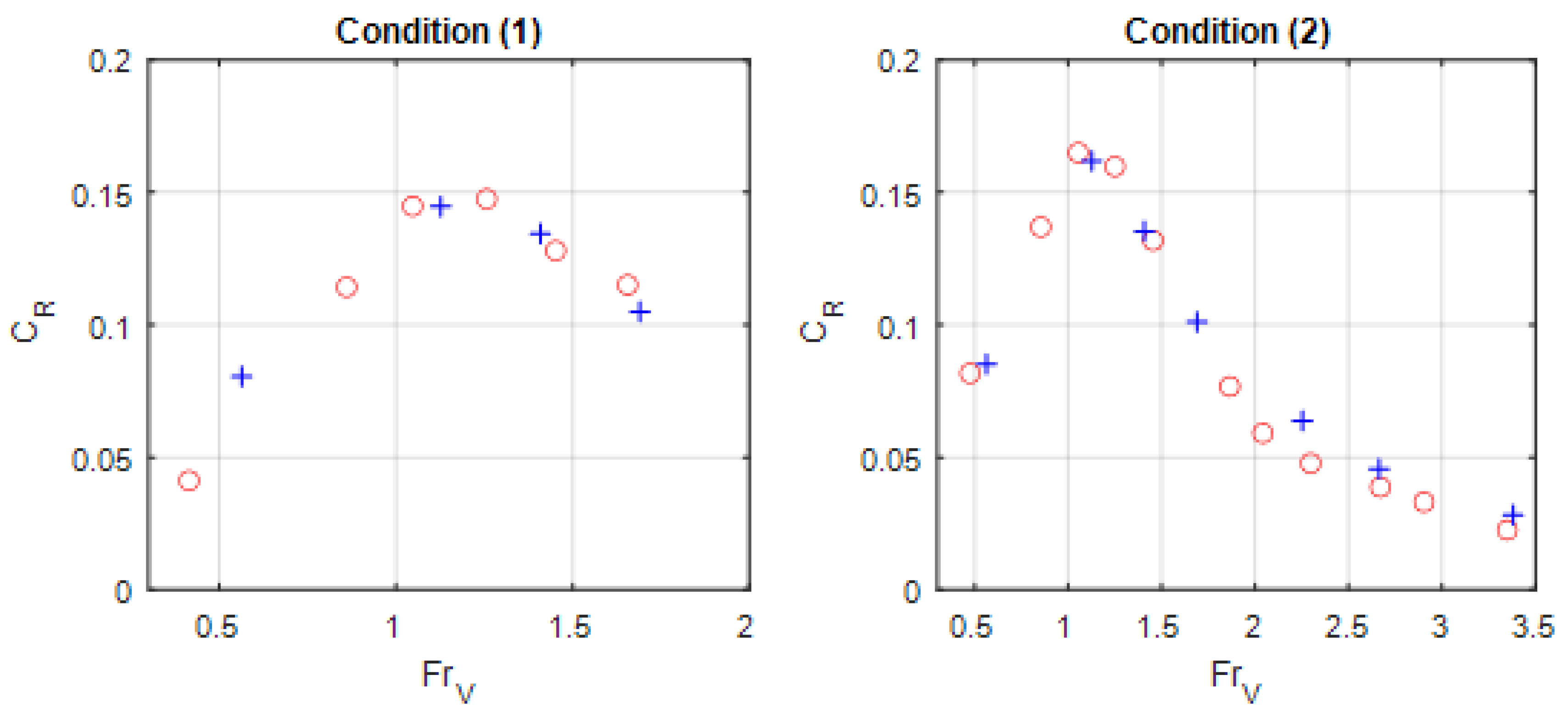
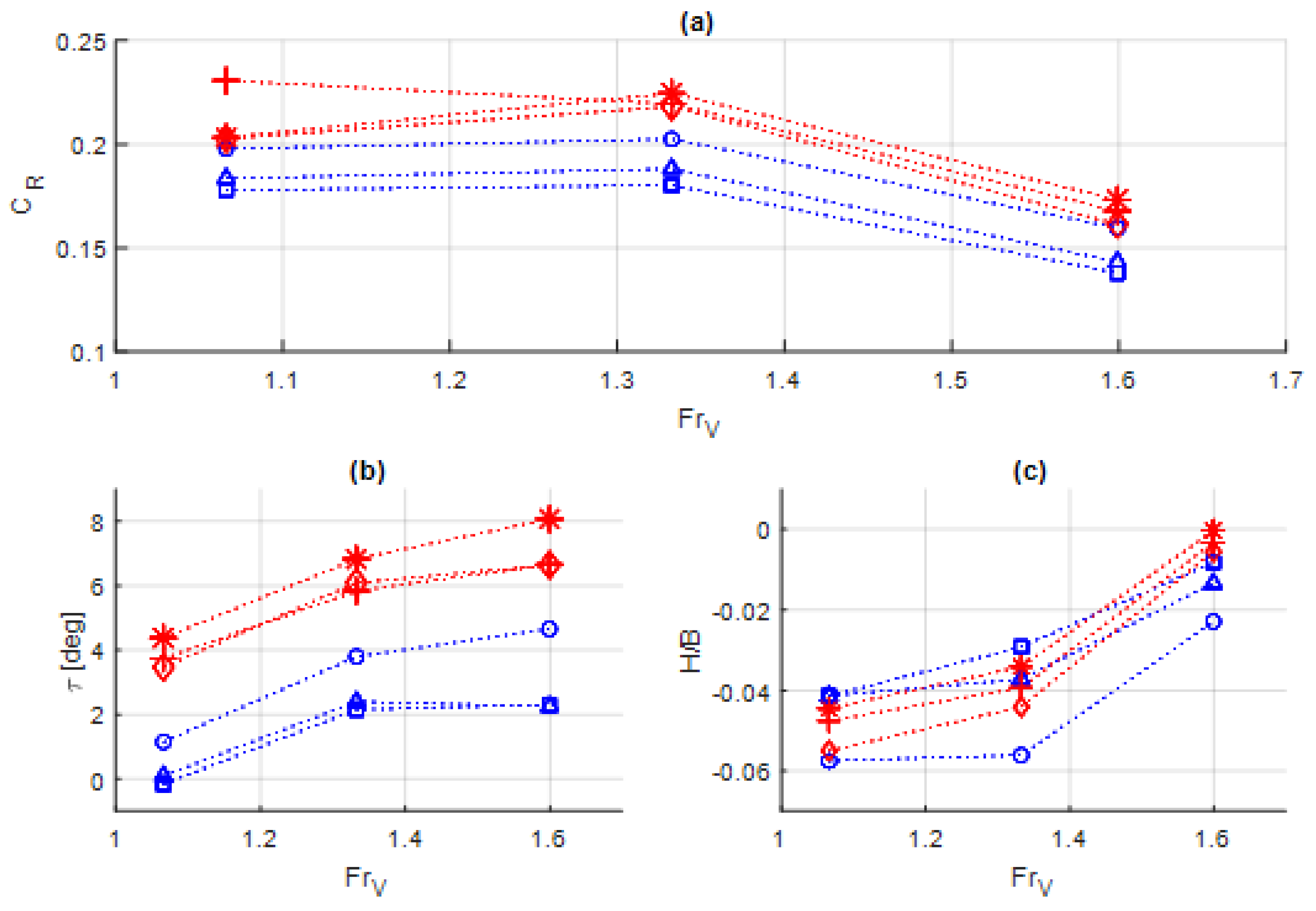
A comparison between numerical and experimental results in the range of speeds for two LCG values is shown in Figure 9. The agreement at transitional speeds, which are the primary interest in this study, is very good. The numerical results show somewhat higher drag than test data in the planing regimes. As stated above, the numerical and experimental uncertainties can be responsible for part of these differences. It is also noted that previous CFD simulations with planing hulls, which employed a much higher number of numerical cells than the present study, produced results demonstrating similar discrepancy with the experimental data [9,10]. Insufficiently accurate modeling of spray at high speeds is a possible cause for this discrepancy. Numerical grids of very high resolution or the development of different models for spray may be needed to address this issue.

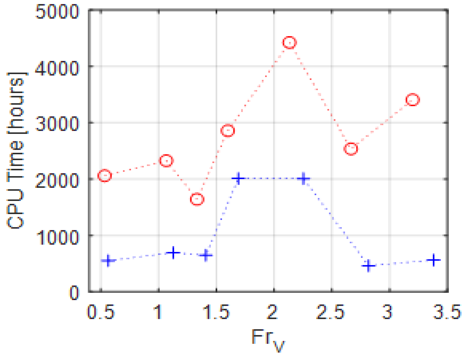
The computational times needed to achieve steady states for the hulls used in the validation study have been assessed as well. The central processing unit (CPU) times, defined as the actual time multiplied by the number of employed processors, is given in Figure 10 for the range of Froude numbers. The heavier hulls and intermediate Froude numbers, which correspond to semi-planing regimes, required longer CPU times.

Additional simulations have been conducted here with different turbulence models on the fine mesh. These models included the $k-\omega$ SST (shear stress transport) and the Reynolds stress turbulence (RST) models. The simulations were carried out for both LCG and Froude numbers used in the verification study. Results for the resistance coefficient are summarized in

Table 2. Resistance coefficient obtained with different turbulence models at two operating conditions.

Turbulence Models	Resistance Coefficient, CR
	Condition (1)	Condition (2)
	LCG = 45%	LCG = 40%
	FrV = 1.67	FrV = 2.68
Realizable $k-\epsilon$	0.110	0.0458
$k-\omega$ SST	0.110	0.0466
Reynolds Stress Turbulence	0.110	0.0485

. The differences in the resistance values were less than 1% for the transitional case, so accuracy of all three turbulence models is about the same at this condition. In the planing regime, the experimental value for $C_R$ was about 0.4, so the error between the experiment and the RST model result was larger and, therefore, the RST model was not used. The realizable $k-\epsilon$ model was chosen since it was closer to the experimental data point and showed lower oscillations in the monitored values compared to the $k-\omega$ SST values.

5. Parametric Results

Since the focus of this study is on heavy hulls that perform well in the transitional speed range, the initial parametric calculations were carried for three hull geometries at the loading coefficient $C_B$ = 1.276, two centers of gravity LCG = 40% and 45%, and speeds corresponding to $F{r}_V$ = 1.0–1.6. To present results in the non-dimensional form, three metrics are used: the resistance coefficient defined by Equation (10), the hull trim, $\tau$, and the rise of the center of gravity (in comparison with the rest position) normalized by the hull beam, $H/B.$

The resistance coefficient and attitude data obtained for heavy hulls in the transitional regime are shown in Figure 11. As one can notice, the hulls with LCG = 45% consistently outperform those with LCG = 40% (Figure 11a). The trim angles of the configurations with the rearward CG are noticeably higher (by 3–4 degrees) than trims of the hull with more forward CG (Figure 11b). At moderate speeds, excessive trim angles result in larger pressure drag, while the hydrodynamic lift is not yet developed to raise these hulls to higher positions. On the contrary, the dynamic suction at these speeds increases the hull submergences. Differences between sinkages of hulls with different CG locations are not as pronounced as differences in drag and trim (Figure 11c). Thus, the hull configurations with LCG = 45% were selected for further studies in a broader speed range.

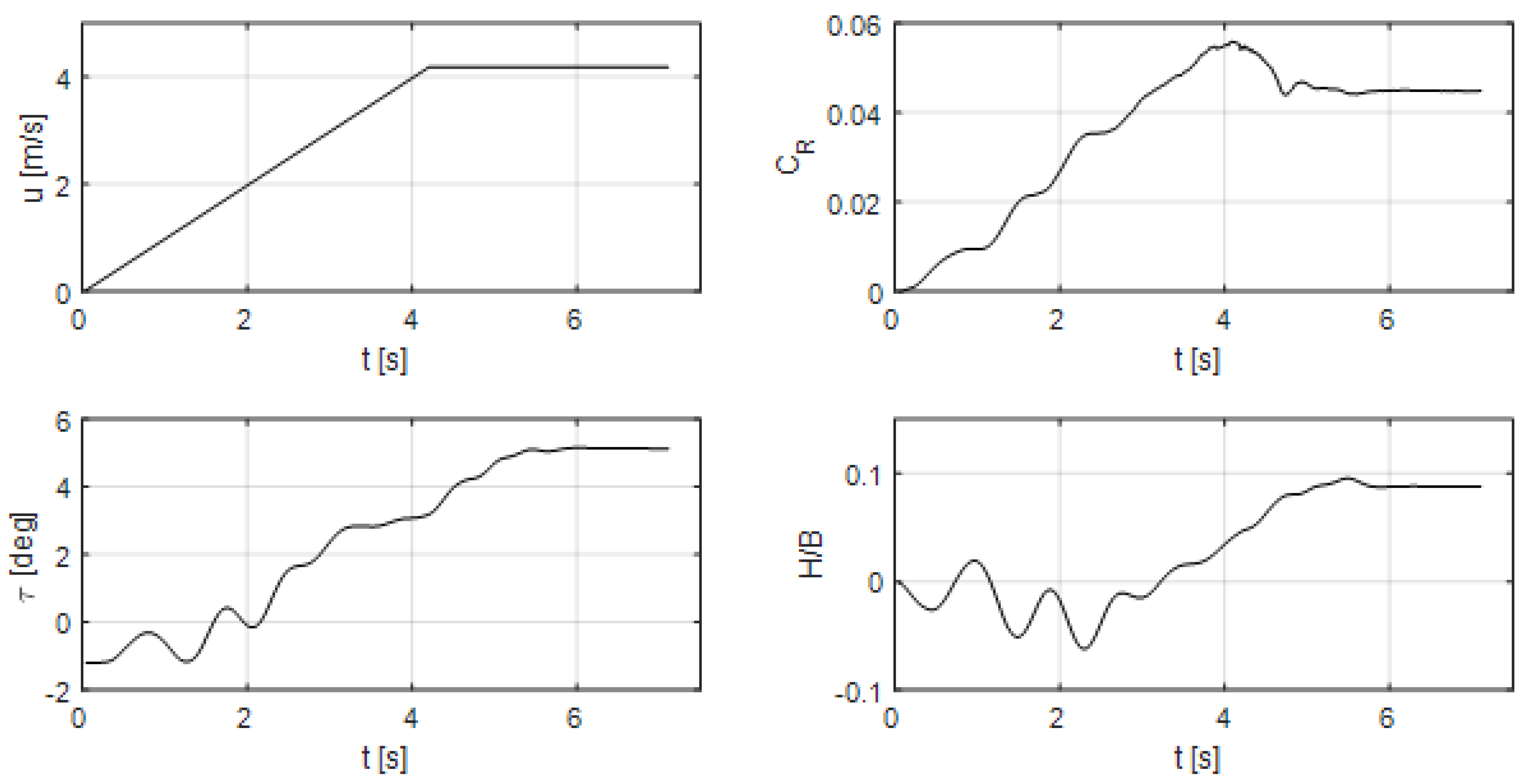
Both nominal and heavy hulls with $C_B$ = 0.912 and 1.276 and three bow geometries were computationally simulated in $F{r}_V$ interval from 0.5 up to 3.5, covering all important regimes from the displacement to planing modes. Starting from zero speed, hulls were accelerated at 1 m/s² till their speeds reached required values. 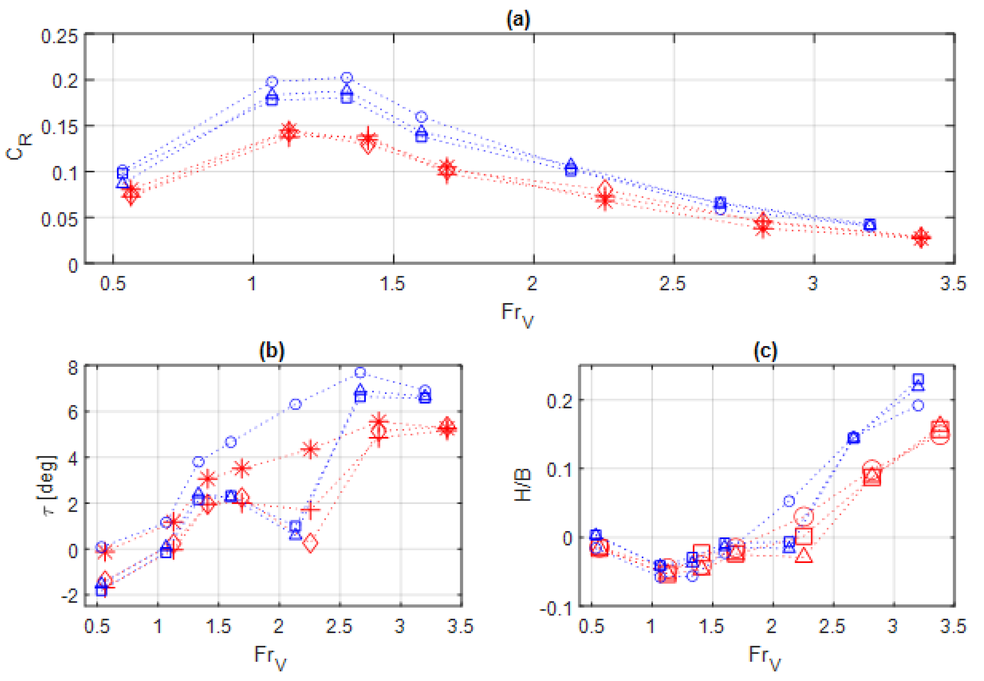An example of time-dependent hull characteristics, demonstrating attainment of a steady-state regime, is shown in Figure 12 for one of the studied hulls. The steady-state results for the resistance coefficient, trim and CG rise for all hull configurations are summarized in Figure 13. General shapes of the resistance coefficient curves (Figure 13a) are rather common to hard-chine hulls. There is a steep drag increase at the transitional speeds, followed by the resistance coefficient peak around $F{r}_V$ = 1.2 and some reduction of resistance at the post-hump planing speeds. As expected, heavy hulls demonstrate higher drag, and the drag increase is roughly similar to the relative increase of hull displacements.

The trim angles generally increase with speed (Figure 13b), demonstrating faster growth at the transitional speeds and saturation at the high planing speeds. However, the hulls with curved bows (both nominal-weight and heavy) exhibit a significant drop in trim at $F{r}_V$ = 2.2. This is caused by earlier exits of finer bows at this speed (in comparison with the original constant deadrise hulls), accompanied by the loss of lift at the front portion of the hull, which results in the bow-down adjustment.

The vertical positions of the hulls’ centers of gravity initially descend due to dynamic suction near $F{r}_V$ = 1.2 but, later, with increasing trim and speed, the hulls rise due to higher hydrodynamic lift (Figure 13c). Again, at $F{r}_V$ = 2.2, the hulls with finer bows do not experience significant elevation increase (as the constant-deadrise hulls) due to trim reduction and some loss of hydrodynamic lift. At higher speeds, resistance and attitude characteristics of hulls of different geometries approach each other, since the bows almost exit the water and the rear prismatic-type hull portions are identical for all three hulls studied here.

When comparing the performance of different hull forms in the overloaded condition, one can notice that the hull with concave bow has consistently lower resistance in the transitional regime, $F{r}_V$= 1.0–1.7. Its finest bow shape (Figure 3), among those of the hulls studied here, helps this hull cut through the water more efficiently at semi-displacement speeds. At the nominal (lighter) loading and lower speeds, $F{r}_V$ < 1.0, the hull with concave bow is also superior in terms of resistance, which will allow it to operate more economically in that regime. When a high speed is needed at the nominal loading, the concave-bow hull will be able to reach planing speeds $F{r}_V$ > 2.5 with the available thrust-weight ratio of 0.2. Thus, the hull with the concave bow would be the best performer for the specific operational regimes of interest to this study. It should be noted that only calm-water conditions were considered here, and additional studies will be needed if operations in rough seas are taken into consideration.

The convex-bow hull (Figure 3), while inferior to the concave counterpart in calm water, slightly outperforms the constant-deadrise hull in the transitional regimes (Figure 13). However, the hull with convex bow exhibits the largest peak of the actual drag force near $F{r}_V$ = 2.2 in both nominal and heavy loadings. The constant-deadrise hull is superior at the planing speeds due to its pronounced prismatic hull surfaces. Again, if operations in waves are considered, relative performances of different hull forms may change.

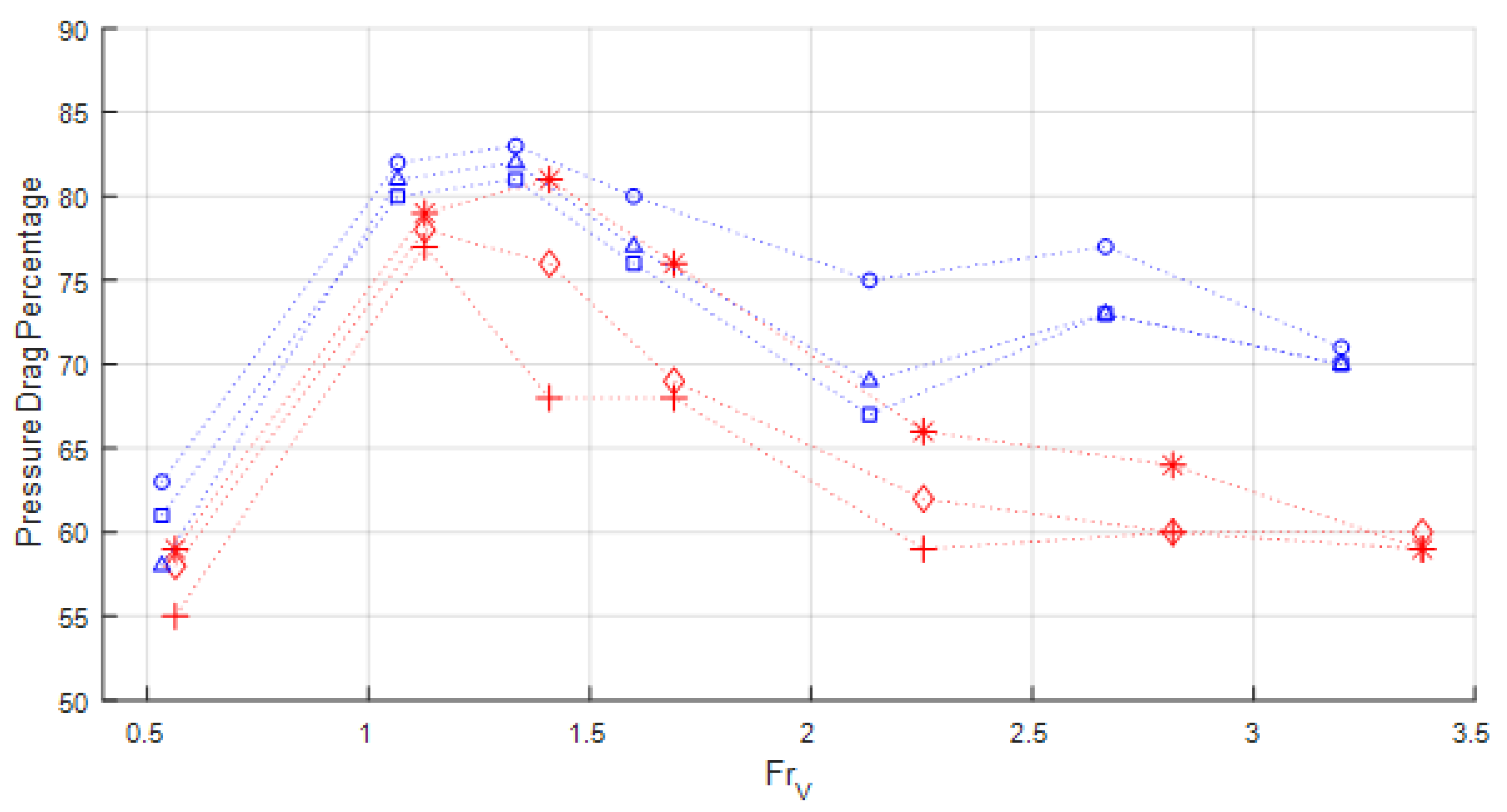
One of the interesting metrics of hulls intended for a broad speed range is the correspondence between pressure and friction (shear) drag components. The fraction of the pressure drag in the total hull resistance is shown in Figure 14. Obviously, heavily loaded hulls have a higher pressure drag contribution in comparison with lighter hulls. The pressure-drag fraction peaks at Froude number around 1.3. These speeds belong to the transitional regime where the hulls experience large drag but relatively low hydrodynamic lift. The secondary peak in the pressure-drag fraction is noticeable for heavy hulls at early planing speeds, $F{r}_V$ = 2.7. As commonly known, the frictional drag becomes more pronounced at the lowest (displacement) and highest (developed planing) speeds (Figure 14), although hulls with the finer bows also tend to have a larger frictional contribution at $F{r}_V$ = 2.2, when hull trim angles drop slightly (Figure 13b).

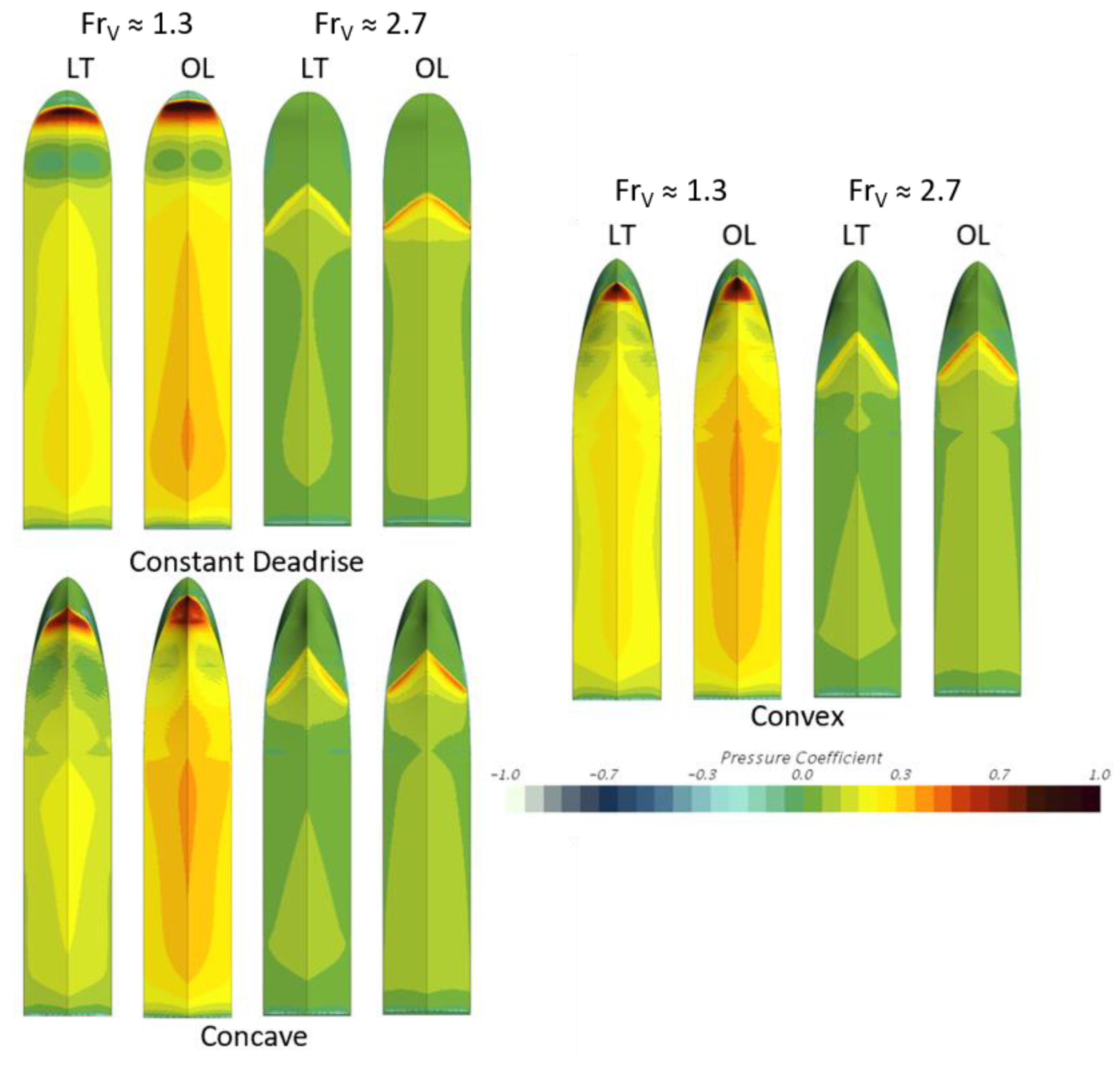
More detailed insight on the flow characteristics near hulls can be gained from the distribution of pressure coefficients, $C_p$, on the hull bottom and the water surface deformations around hulls, which are given for selected states in Figure 15 and Figure 16, respectively. One can notice a slightly larger wet area of a constant-deadrise hull bottom at the lower speed ($F{r}_V$ ≈ 1.3) in comparison with other hulls that have finer bows (Figure 15). The highest pressure coefficient is observed at the water impingement zone at the bow. In the overloaded cases and lower speeds, this high-pressure zone is more pronounced for the constant-deadrise hull (Figure 15), while $C_p$ magnitudes in this region are the lowest for the concave-bow hull. This is consistent with the resistance coefficient values shown in Figure 13a, where the constant-deadrise and concave-bow heavy hulls have the highest and lowest resistances, respectively, at $F{r}_V$ ≈ 1.3. On the other hand, small regions with reduced pressure are visible near hull transoms, where pressure recovers back to atmospheric and, therefore, does not significantly contribute to the boat lift. At $F{r}_V$ ≈ 2.7, pressure coefficient values are generally smaller since the flow speeds are higher, but loadings are the same. The wet area of the constant-deadrise hull is smaller at higher speed ($F{r}_V$ ≈ 2.7) than wet areas of concave- and convex-bow hulls due to larger trim angles of the constant-deadrise hull (Figure 13b).

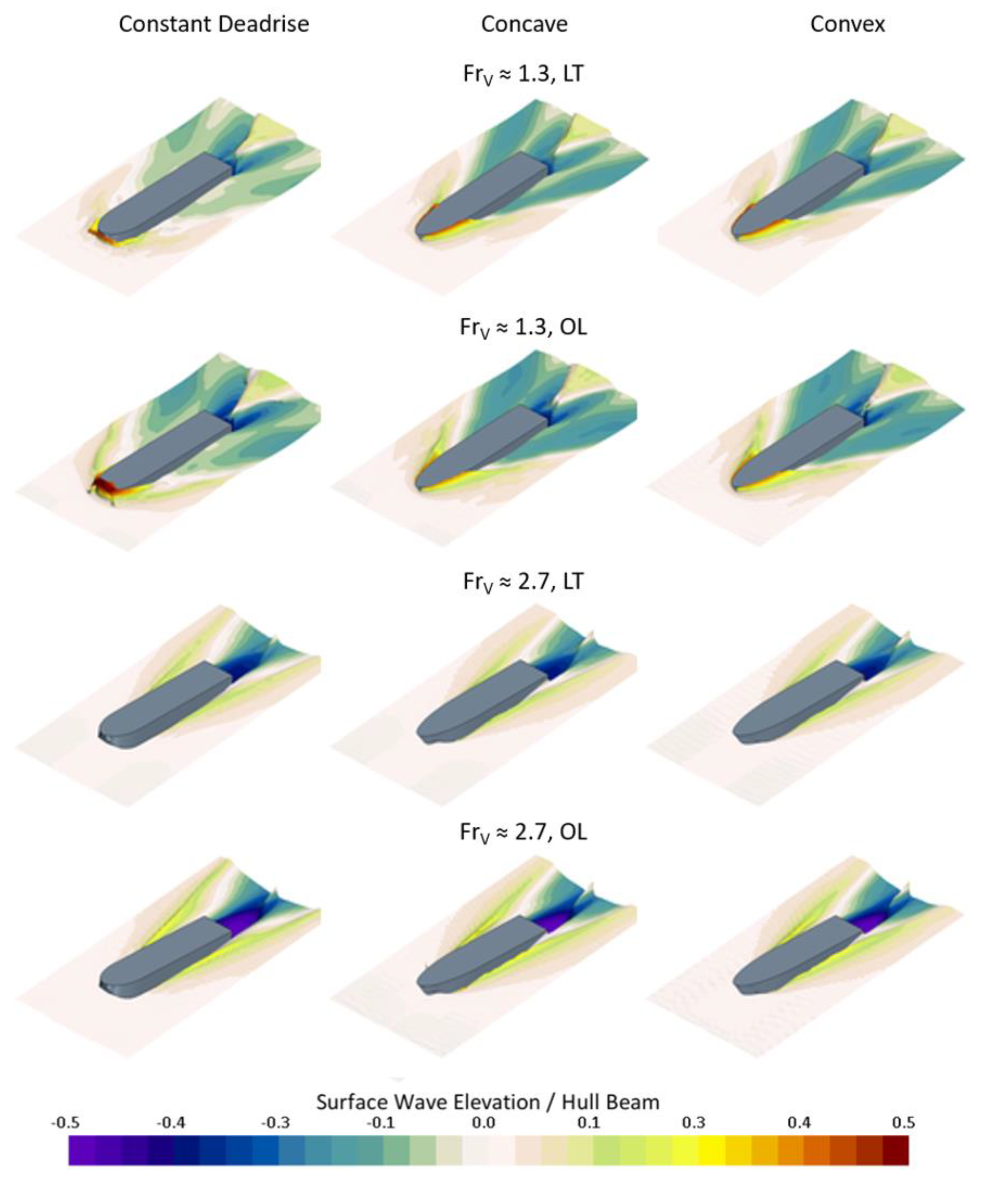
The near-hull water surface elevations for the same 12 cases are illustrated in Figure 16. At lower speeds ($F{r}_V$ ≈ 1.3), significant water build-up with wave breaking features appears in front of the bow of the constant-deadrise hull, whereas the bow waves extend further along the hulls with finer bows. The concave-hull bow nose is slightly less wet than the convex-hull counterpart. The water depression at the transom and the following “rooster tail” are more pronounced for heavier hulls. At higher speed ($F{r}_V$ ≈ 2.7), the constant deadrise-hull has a noticeably larger trim than other hulls. The “rooster tails” of convex and concave hulls are located closer to the transom than for a more prismatic hull. The divergent waves generated by heavier hulls are more pronounced, since those hulls displace more water. The wake zones of faster hulls are narrower than those behind hulls operating at lower speeds. The water depression zones behind the transom become more aligned with the hull centerline at higher speeds in comparison with wave hollows nearly split in two parts behind most hulls at lower speeds.

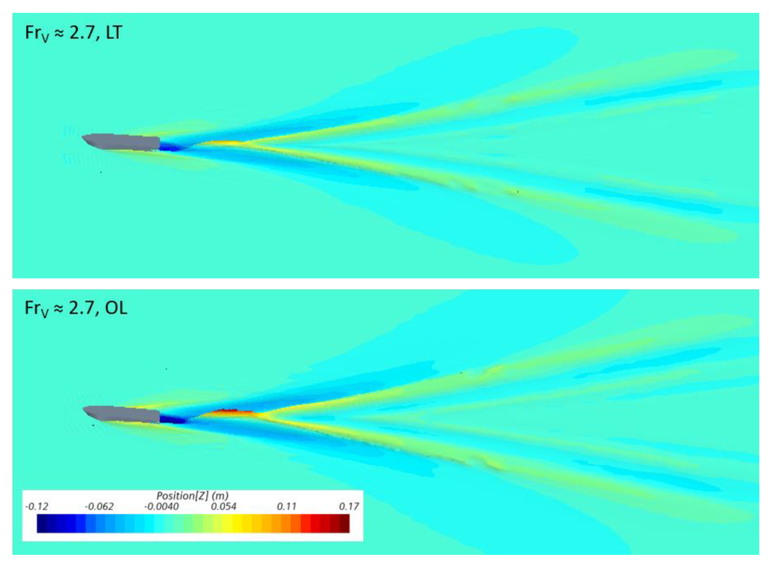
The full-domain wave patterns behind one of the hulls at two loadings are illustrated in Figure 17. At this high speed ($F{r}_V$ ≈ 2.7), the well-defined divergent waves are clearly visible. The heavier hull sits deeper in the water and produces larger wave amplitudes. Near the downstream boundary on the right side of computational domains in Figure 17, the numerical forcing zone suppresses the waves, resulting in diminishing magnitudes of water surface elevations.

6. Conclusions

A computational study has been undertaken to evaluate the performance of basic hard-chine hull forms in heavily loaded conditions and in the broad speed range from the displacement to planing regimes. The resistance coefficient curves demonstrated a typical behavior with the peaks around the displacement Froude number of 1.2. Hulls with 40% heavier displacements manifested about 30% larger resistance than lighter hulls over the studied speed range. In the overloaded regime and transitional speeds, the concave-bow hull is found to have about 5% and 12% lower drag than the convex-bow hull and the more prismatic constant-deadrise hull, respectively. The same convex-bow hull at the nominal loading and displacement speeds showed 2–10% lower drag than the other hulls, as well as moderate resistance up to the planing speeds. The hulls with finer bows exhibited a significant 2–3° trim decrease at the hump speed. The original constant-deadrise hull with a long prismatic portion of the hull performs better at the planing speeds, demonstrating 5–15% lower drag than other hulls.

Future research directions can involve investigating the performance of heavy hulls in the presence of waves to provide recommendations for overloaded hard-chine hulls intended for variable sea conditions. The present computational approach is also suitable for determining the effects of finer geometric details on the hull surfaces, such as spray rails, steps, and appendages, and conducting hull optimization studies at the design stage.