
Deep Learning for Deep Waters: An Expert-in-the-Loop Machine Learning Framework for Marine Sciences

 , , and
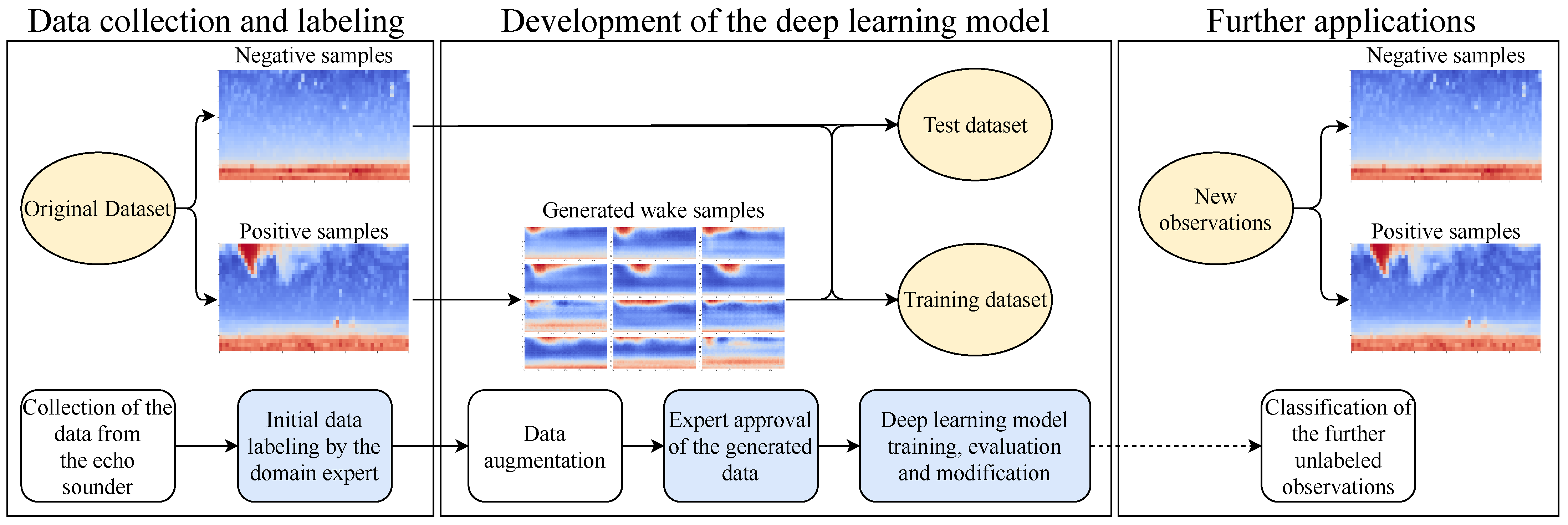
Abstract
1. Introduction
2. Background: Bridging Machine Learning and Marine Science
2.1. Deep Learning for Signal and Image Analysis
2.2. Machine Learning for Acoustic Detection in Marine Science
3. Materials and Methods
- In situ collection of acoustic data (Section 3.4);
- Initial data labelling by the domain expert (Section 3.5);
- Data augmentation and its approval by the expert (Section 3.6);
- Training baseline deep learning model (Section 3.7);
- Evaluating baseline model’s performance (Section 3.8);
- Implementing algorithms to make the model robust against data imbalance and noise with an additional input from the expert (Section 3.7 and Section 3.8);
- Evaluating the final model (Section 4).
3.1. Expert-in-the-Loop
3.2. Machine Learning: Classification
3.2.1. Convolutional Neural Network
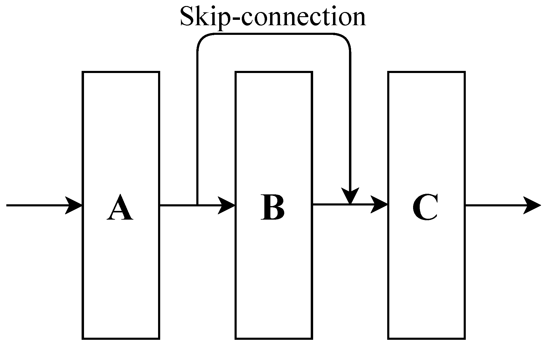
3.2.2. Residual Neural Network
3.3. Approaches for Scarce Data
3.3.1. Data Augmentation
3.3.2. Probabilistic Models
3.4. In-Situ Data Collection
3.4.1. ADCP Measurements
3.4.2. AIS Data
3.5. Data Labelling and Preparation
3.5.1. Data Labelling
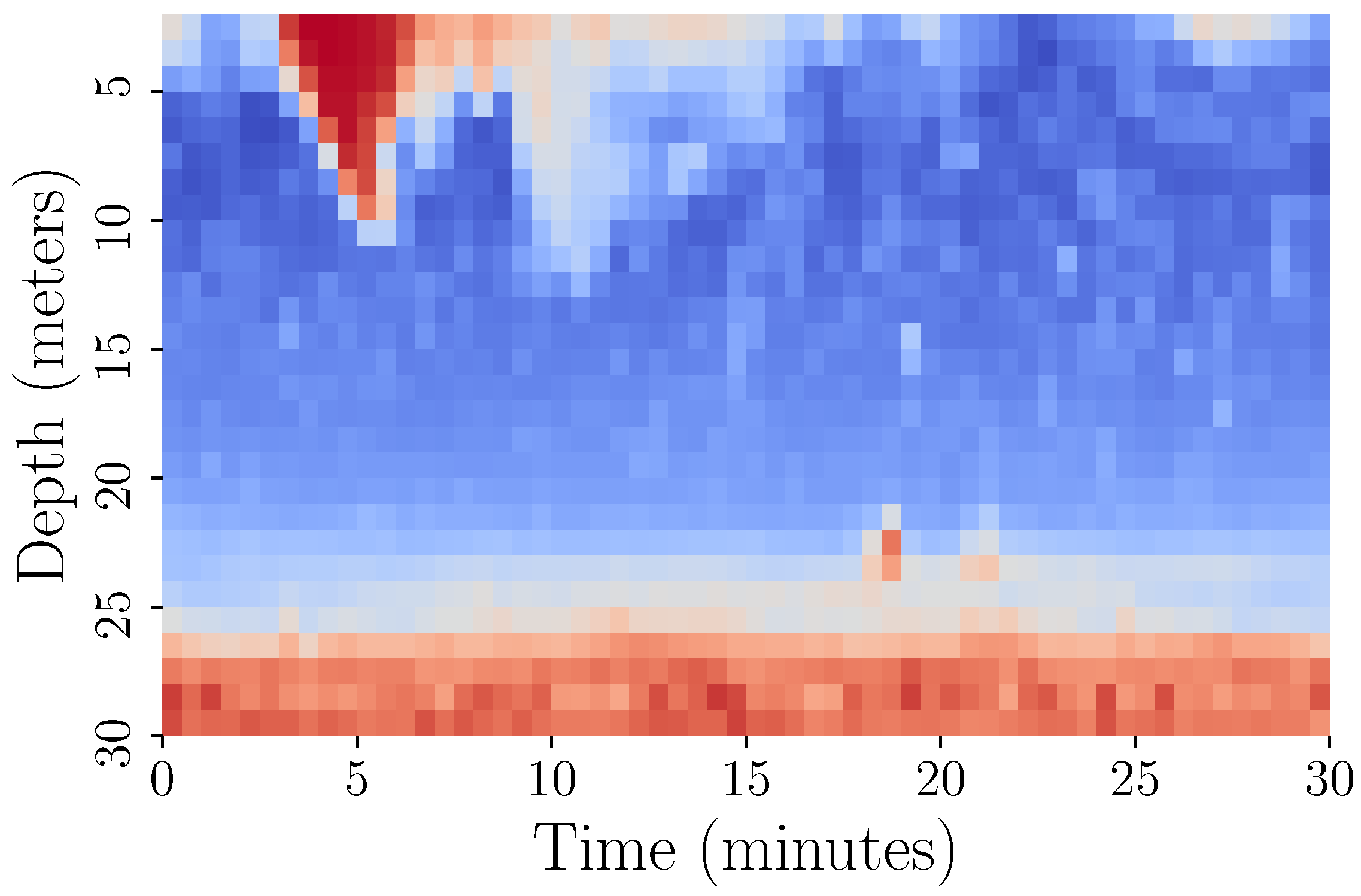
3.5.2. Data Representation and Visualisation
3.5.3. Set-Aside Dataset
3.6. Data Augmentation
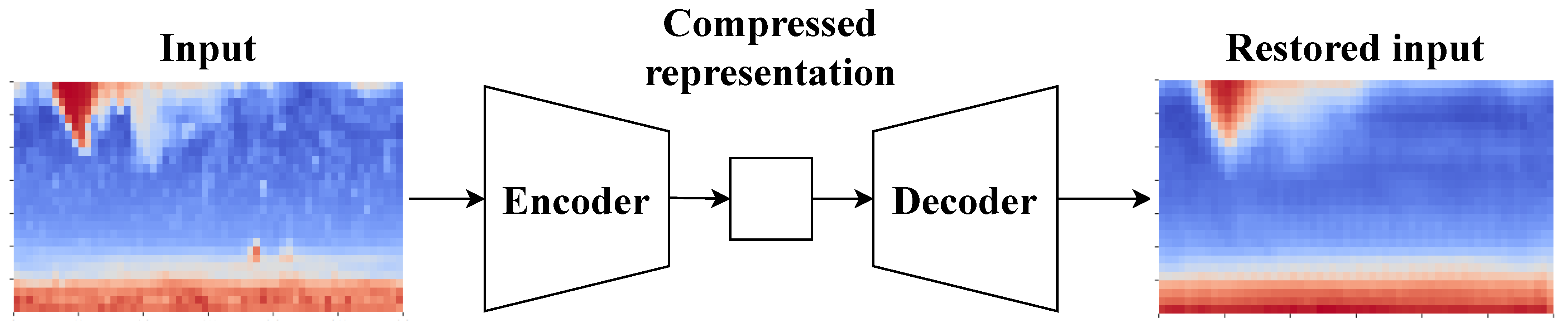
3.6.1. Data Compression
3.6.2. Sample Generation
3.7. Deep Learning Models
3.8. Evaluation Metrics
4. Results
4.1. Baseline ResNet Model
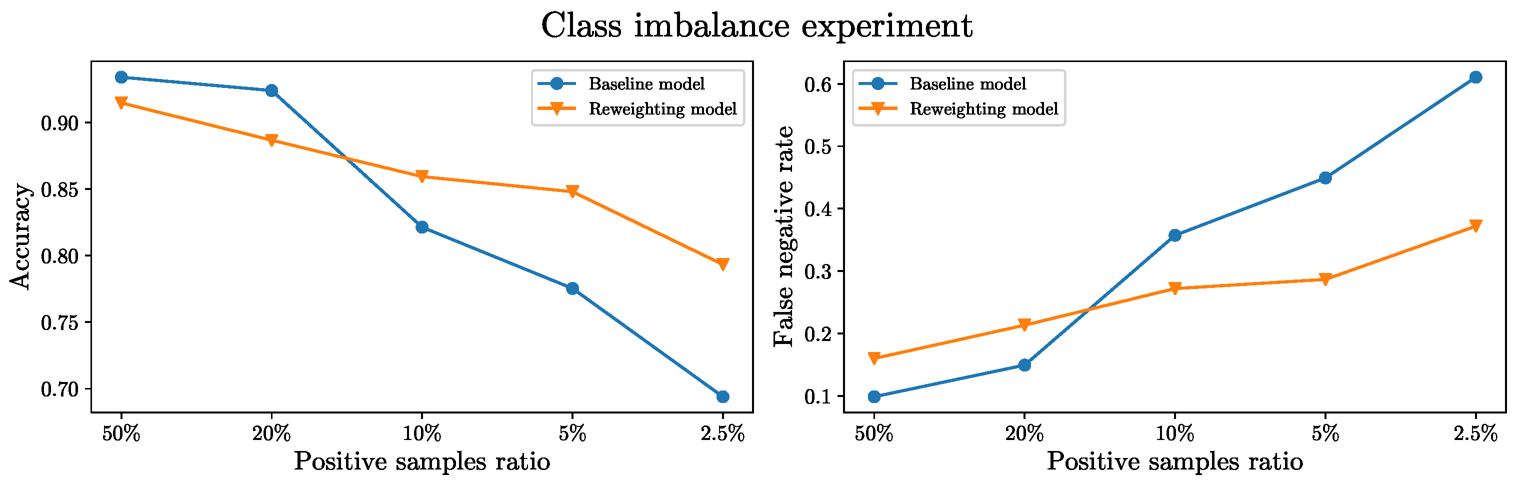
4.2. Example Reweighting Model
4.3. Set-Aside Dataset Experiment
5. Discussion
6. Conclusions
Author Contributions
Funding
Institutional Review Board Statement
Informed Consent Statement
Data Availability Statement
Acknowledgments
Conflicts of Interest
Abbreviations
| ADCP | Acoustic Doppler Current Profiler |
| AI | Artificial Intelligence |
| AIC | Akaike Information Criterion |
| AIS | Automatic Information System |
| ANN | Artificial Neural Networks |
| AUC ROC | Area Under Receiver Operating Characteristic Curve |
| CNN | Convolutional Neural Networks |
| EMB | European Marine Board |
| EMODnet | The European Marine Observation and Data Network |
| EU | European Union |
| FNR | False Negative Rate |
| GAN | Generative Adversarial Network |
| GMM | Gaussian Mixture Model |
| HELCOM | Baltic Marine Environment Protection Commission |
| IOC | Intergovernmental Oceanographic Commission |
| ML | Machine Learning |
| MSFD | Marine Strategy Framework Directive |
| PCA | Principal Component Analysis |
| ResNet | Residual Neural Network |
| SIME | Swedish Institute for the Marine Environment |
| UN | United Nations |
| VGG | Visual Geometry Group |
References
- Guidi, L.; Fernandez Guerra, A.; Canchaya, C.; Curry, E.; Foglini, F.; Irisson, J.O.; Malde, K.; Marshall, C.T.; Obst, M.; Ribeiro, R.P.; et al. Big Data in Marine Science; Future Science Brief 6 of the European Marine Board: Ostend, Belgium, 2020. [Google Scholar]
- Malde, K.; Handegard, N.O.; Eikvil, L.; Salberg, A.B. Machine intelligence and the data-driven future of marine science. ICES J. Mar. Sci. 2020, 77, 1274–1285. [Google Scholar] [CrossRef]
- Intergovernmental Oceanographic Commission (IOC). The Science we Need for the Ocean We Want: The United Nations Decade of Ocean Science for Sustainable Development (2021–2030); (English) IOC Brochure 2018-7 (IOC/BRO/2018/7 Rev); IOC: Paris, France, 2019; 24p.
- GOOS. Global Ocean Observing System-GOOS. 2020. Available online: https://www.goosocean.org/ (accessed on 22 June 2020).
- The European Marine Observation and Data Network (EMODnet). Central Portal|Your Gateway to Marine Data in Europe. 2020. Available online: https://www.emodnet.eu/ (accessed on 22 June 2020).
- Copernicus-The European Earth Observation Programme. Copernicus-Marine Environment Monitoring Service. 2020. Available online: https://marine.copernicus.eu/ (accessed on 22 June 2020).
- Allken, V.; Handegard, N.O.; Rosen, S.; Schreyeck, T.; Mahiout, T.; Malde, K. Fish species identification using a convolutional neural network trained on synthetic data. ICES J. Mar. Sci. 2018, 76, 342–349. [Google Scholar] [CrossRef]
- Horne, J.K. Acoustic approaches to remote species identification: A review. Fish. Oceanogr. 2000, 9, 356–371. [Google Scholar] [CrossRef]
- Godø, O.R.; Handegard, N.O.; Browman, H.I.; Macaulay, G.J.; Kaartvedt, S.; Giske, J.; Ona, E.; Huse, G.; Johnsen, E. Marine ecosystem acoustics (MEA): Quantifying processes in the sea at the spatio-temporal scales on which they occur. ICES J. Mar. Sci. 2014, 71, 2357–2369. [Google Scholar] [CrossRef]
- Benoit-Bird, K.J.; Lawson, G.L. Ecological Insights from Pelagic Habitats Acquired Using Active Acoustic Techniques. Annu. Rev. Mar. Sci. 2016, 8, 463–490. [Google Scholar] [CrossRef]
- Bennion, M.; Fisher, J.; Yesson, C.; Brodie, J. Remote Sensing of Kelp (Laminariales, Ochrophyta): Monitoring Tools and Implications for Wild Harvesting. Rev. Fish. Sci. Aquac. 2019, 27, 127–141. [Google Scholar] [CrossRef]
- Zampoukas, N.; Palialexis, A.; Duffek, A.; Graveland, J.; Giorgi, G.; Hagebro, C.; Hanke, G.; Korpinen, S.; Tasker, M.; Tornero, V.; et al. Technical Guidance on Monitoring for the Marine Strategy Framework Directive; Publications Office of the European Union: Luxembourg, 2014; ISSN 831-9424. ISBN 978-92-79-35426-7. [Google Scholar]
- Brown, C.J.; Smith, S.J.; Lawton, P.; Anderson, J.T. Benthic habitat mapping: A review of progress towards improved understanding of the spatial ecology of the seafloor using acoustic techniques. Estuar. Coast. Shelf Sci. 2011, 92, 502–520. [Google Scholar] [CrossRef]
- Gumusay, M.U.; Bakirman, T.; Tuney Kizilkaya, I.; Aykut, N.O. A review of seagrass detection, mapping and monitoring applications using acoustic systems. Eur. J. Remote Sens. 2019, 52, 1–29. [Google Scholar] [CrossRef]
- Misund, O.A. Underwater acoustics in marine fisheries and fisheries research. Rev. Fish Biol. Fish. 1997, 7, 1–34. [Google Scholar] [CrossRef]
- Ross, T.; Gaboury, I.; Lueck, R. Simultaneous acoustic observations of turbulence and zooplankton in the ocean. Deep. Sea Res. Part I Oceanogr. Res. Pap. 2007, 54, 143–153. [Google Scholar] [CrossRef]
- Lombard, F.; Boss, E.; Waite, A.M.; Vogt, M.; Uitz, J.; Stemmann, L.; Sosik, H.M.; Schulz, J.; Romagnan, J.B.; Picheral, M.; et al. Globally Consistent Quantitative Observations of Planktonic Ecosystems. Front. Mar. Sci. 2019, 6, 196. [Google Scholar] [CrossRef]
- Williamson, B.J.; Blondel, P.; Armstrong, E.; Bell, P.S.; Hall, C.; Waggitt, J.J.; Scott, B.E. A self-contained subsea platform for acoustic monitoring of the environment around Marine Renewable Energy Devices-Field deployments at wave and tidal energy sites in Orkney, Scotland. IEEE J. Ocean. Eng. 2015, 41, 67–81. [Google Scholar]
- Francisco, F.; Sundberg, J. Detection of Visual Signatures of Marine Mammals and Fish within Marine Renewable Energy Farms using Multibeam Imaging Sonar. J. Mar. Sci. Eng. 2019, 7, 22. [Google Scholar] [CrossRef]
- Stranne, C.; Mayer, L.; Jakobsson, M.; Weidner, E.; Jerram, K.; Weber, T.C.; Anderson, L.G.; Nilsson, J.; Björk, G.; Gårdfeldt, K. Acoustic mapping of mixed layer depth. Ocean Sci. 2018, 14, 503–514. [Google Scholar] [CrossRef]
- Stranne, C.; Mayer, L.; Weber, T.C.; Ruddick, B.R.; Jakobsson, M.; Jerram, K.; Weidner, E.; Nilsson, J.; Gårdfeldt, K. Acoustic mapping of thermohaline staircases in the arctic ocean. Sci. Rep. 2017, 7, 1–9. [Google Scholar] [CrossRef]
- Lavery, A.C.; Geyer, W.R.; Scully, M.E. Broadband acoustic quantification of stratified turbulence. J. Acoust. Soc. Am. 2013, 134, 40–54. [Google Scholar] [CrossRef] [PubMed]
- European Parliament. Directive 2008/56/EC of the European Parliament and of the Council of 17 June 2008 establishing a framework for community action in the field of marine environmental policy (Marine Strategy Framework Directive). Off. J. Eur. Union L 2008, 164, 19–40. [Google Scholar]
- Kelpšaite, L.; Parnell, K.; Soomere, T. Energy pollution: The relative influence of wind-wave and vessel-wake energy in Tallinn Bay, the Baltic Sea. J. Coast. Res. 2009, 56, 812–816. [Google Scholar]
- Zaggia, L.; Lorenzetti, G.; Manfé, G.; Scarpa, G.M.; Molinaroli, E.; Parnell, K.E.; Rapaglia, J.P.; Gionta, M.; Soomere, T. Fast shoreline erosion induced by ship wakes in a coastal lagoon: Field evidence and remote sensing analysis. PLoS ONE 2017, 12, e0187210. [Google Scholar] [CrossRef] [PubMed]
- NDRC. The Physics of Sound in the Sea; United States Office of Scientific Research and Development, National Defense Research Committee, Division 6: Washington, DC, USA, 1946. Available online: https://www.loc.gov/item/2015490953/ (accessed on 27 April 2020).
- Soloviev, A.; Gilman, M.; Young, K.; Brusch, S.; Lehner, S. Sonar measurements in ship wakes simultaneous with TerraSAR-X overpasses. IEEE Trans. Geosci. Remote Sens. 2010, 48, 841–851. [Google Scholar] [CrossRef]
- Voropayev, S.; Nath, C.; Fernando, H. Thermal surface signatures of ship propeller wakes in stratified waters. Phys. Fluids 2012, 24, 116603. [Google Scholar] [CrossRef]
- Francisco, F.; Carpman, N.; Dolguntseva, I.; Sundberg, J. Use of Multibeam and Dual-Beam Sonar Systems to Observe Cavitating Flow Produced by Ferryboats: In a Marine Renewable Energy Perspective. J. Mar. Sci. Eng. 2017, 5, 30. [Google Scholar] [CrossRef]
- Trevorrow, M.V.; Vagle, S.; Farmer, D.M. Acoustical measurements of microbubbles within ship wakes. J. Acoust. Soc. Am. 1994, 95, 1922–1930. [Google Scholar] [CrossRef]
- Weber, T.C.; Lyons, A.P.; Bradley, D.L. An estimate of the gas transfer rate from oceanic bubbles derived from multibeam sonar observations of a ship wake. J. Geophys. Res. Ocean. 2005, 110. [Google Scholar] [CrossRef]
- Emerson, S.; Bushinsky, S. The role of bubbles during air-sea gas exchange. J. Geophys. Res. Ocean. 2016, 121, 4360–4376. [Google Scholar] [CrossRef]
- Uliczka, K.; Kondziella, B. Ship-Induced Sediment Transport in Coastal Waterways (SeST). In Proceedings of the 4th MASHCON-International Conference on Ship Manoeuvring in Shallow and Confined Water with Special Focus on Ship Bottom Interaction, Hamburg, Germany, 23–25 May 2016; pp. 2–8. [Google Scholar]
- Katz, C.; Chadwick, D.; Rohr, J.; Hyman, M.; Ondercin, D. Field measurements and modeling of dilution in the wake of a US navy frigate. Mar. Pollut. Bull. 2003, 46, 991–1005. [Google Scholar] [CrossRef][Green Version]
- Loehr, L.C.; Beegle-Krause, C.J.; George, K.; McGee, C.D.; Mearns, A.J.; Atkinson, M.J. The significance of dilution in evaluating possible impacts of wastewater discharges from large cruise ships. Mar. Pollut. Bull. 2006, 52, 681–688. [Google Scholar] [CrossRef]
- Marmorino, G.; Trump, C. Preliminary side-scan ADCP measurements across a ship’s wake. J. Atmos. Ocean. Technol. 1996, 13, 507–513. [Google Scholar] [CrossRef]
- Ermakov, S.A.; Kapustin, I.A. Experimental study of turbulent-wake expansion from a surface ship. Izv. Atmos. Ocean. Phys. 2010, 46, 524–529. [Google Scholar] [CrossRef]
- Kang, L. Wave Monitoring Based on Improved Convolution Neural Network. J. Coast. Res. 2019, 94, 186–190. [Google Scholar] [CrossRef]
- Holzinger, A. Interactive machine learning for health informatics: When do we need the human-in-the-loop? Brain Inform. 2016, 3, 119–131. [Google Scholar] [CrossRef] [PubMed]
- Holzinger, A.; Plass, M.; Holzinger, K.; Crisan, G.C.; Pintea, C.M.; Palade, V. A glass-box interactive machine learning approach for solving NP-hard problems with the human-in-the-loop. Creat. Math. Inform. 2019, 28, 121–134. [Google Scholar]
- Guo, X.; Yu, Q.; Li, R.; Alm, C.O.; Calvelli, C.; Shi, P.; Haake, A. An expert-in-the-loop paradigm for learning medical image grouping. In Pacific-Asia Conference on Knowledge Discovery and Data Mining; Springer: Cham, Switzerland, 2016; pp. 477–488. [Google Scholar]
- Schmidhuber, J. Deep learning in neural networks: An overview. Neural Netw. 2015, 61, 85–117. [Google Scholar] [CrossRef]
- LeCun, Y.; Bengio, Y.; Hinton, G. Deep learning. Nature 2015, 521, 436–444. [Google Scholar] [CrossRef]
- Alexandrou, D.; Pantzartzis, D. A methodology for acoustic seafloor classification. IEEE J. Ocean. Eng. 1993, 18, 81–86. [Google Scholar] [CrossRef]
- Marsh, I.; Brown, C. Neural network classification of multibeam backscatter and bathymetry data from Stanton Bank (Area IV). Appl. Acoust. 2009, 70, 1269–1276. [Google Scholar] [CrossRef]
- Feldens, P.; Darr, A.; Feldens, A.; Tauber, F. Detection of boulders in side scan sonar mosaics by a neural network. Geosciences 2019, 9, 159. [Google Scholar] [CrossRef]
- van Overmeeren, R.; Craeymeersch, J.; van Dalfsen, J.; Fey, F.; van Heteren, S.; Meesters, E. Acoustic habitat and shellfish mapping and monitoring in shallow coastal water—Sidescan sonar experiences in The Netherlands. Estuar. Coast. Shelf Sci. 2009, 85, 437–448. [Google Scholar] [CrossRef]
- Lawson, G.L.; Barange, M.; Fréon, P. Species identification of pelagic fish schools on the South African continental shelf using acoustic descriptors and ancillary information. ICES J. Mar. Sci. 2001, 58, 275–287. [Google Scholar] [CrossRef]
- Korneliussen, R.J.; Heggelund, Y.; Macaulay, G.J.; Patel, D.; Johnsen, E.; Eliassen, I.K. Acoustic identification of marine species using a feature library. Methods Oceanogr. 2016, 17, 187–205. [Google Scholar] [CrossRef]
- Williamson, B.J.; Fraser, S.; Blondel, P.; Bell, P.S.; Waggitt, J.J.; Scott, B.E. Multisensor Acoustic Tracking of Fish and Seabird Behavior Around Tidal Turbine Structures in Scotland. IEEE J. Ocean. Eng. 2017, 42, 948–965. [Google Scholar] [CrossRef]
- Fraser, S.; Nikora, V.; Williamson, B.J.; Scott, B.E. Automatic active acoustic target detection in turbulent aquatic environments. Limnol. Oceanogr. Methods 2017, 15, 184–199. [Google Scholar] [CrossRef]
- Fernandes, P.G. Classification trees for species identification of fish-school echotraces. ICES J. Mar. Sci. 2009, 66, 1073–1080. [Google Scholar] [CrossRef]
- Haralabous, J.; Georgakarakos, S. Artificial neural networks as a tool for species identification of fish schools. ICES J. Mar. Sci. 1996, 53, 173–180. [Google Scholar] [CrossRef]
- Simmonds, J.E.; Armstrong, F.; Copland, P.J. Species identification using wideband backscatter with neural network and discriminant analysis. ICES J. Mar. Sci. 1996, 53, 189–195. [Google Scholar] [CrossRef]
- Ramani, N.; Patrick, P.H. Fish detection and identification using neural networks-some laboratory results. IEEE J. Ocean. Eng. 1992, 17, 364–368. [Google Scholar] [CrossRef]
- Cabreira, A.G.; Tripode, M.; Madirolas, A. Artificial neural networks for fish-species identification. ICES J. Mar. Sci. 2009, 66, 1119–1129. [Google Scholar] [CrossRef]
- Brautaset, O.; Waldeland, A.U.; Johnsen, E.; Malde, K.; Eikvil, L.; Salberg, A.B.; Handegard, N.O. Acoustic classification in multifrequency echosounder data using deep convolutional neural networks. ICES J. Mar. Sci. 2020, 77, 1391–1400. [Google Scholar] [CrossRef]
- Krizhevsky, A.; Sutskever, I.; Hinton, G.E. Imagenet classification with deep convolutional neural networks. In Advances in Neural Information Processing Systems; The MIT Press: Cambridge, MA, USA, 2012; pp. 1097–1105. [Google Scholar]
- Simonyan, K.; Zisserman, A. Very deep convolutional networks for large-scale image recognition. arXiv 2014, arXiv:1409.1556. [Google Scholar]
- He, K.; Zhang, X.; Ren, S.; Sun, J. Deep residual learning for image recognition. In Proceedings of the IEEE Conference on Computer Vision and Pattern Recognition, Las Vegas, NV, USA, 27–30 June 2016; pp. 770–778. [Google Scholar]
- Van Dyk, D.A.; Meng, X.L. The art of data augmentation. J. Comput. Graph. Stat. 2001, 10, 1–50. [Google Scholar] [CrossRef]
- Reynolds, D.A. Gaussian Mixture Models. Encycl. Biom. 2009, 741, 659–663. [Google Scholar]
- Hurvich, C.M.; Simonoff, J.S.; Tsai, C.L. Smoothing parameter selection in nonparametric regression using an improved Akaike information criterion. J. R. Stat. Soc. Ser. B (Stat. Methodol.) 1998, 60, 271–293. [Google Scholar] [CrossRef]
- Cao, L.; Chua, K.S.; Chong, W.; Lee, H.; Gu, Q. A comparison of PCA, KPCA and ICA for dimensionality reduction in support vector machine. Neurocomputing 2003, 55, 321–336. [Google Scholar] [CrossRef]
- Port of Gothenburg. 2020. Available online: https://www.portofgothenburg.com/FileDownload/?contentReferenceID=12900 (accessed on 18 May 2020).
- HELCOM. HELCOM Assessment on Maritime Activities in the Baltic Sea 2018. Baltic Sea Environment Proceedings No.152. 2018. Available online: https://www.helcom.fi/wp-content/uploads/2019/08/BSEP152-1.pdf (accessed on 14 January 2021).
- Goodfellow, I.; Pouget-Abadie, J.; Mirza, M.; Xu, B.; Warde-Farley, D.; Ozair, S.; Courville, A.; Bengio, Y. Generative adversarial nets. In Advances in Neural Information Processing Systems; The MIT Press: Cambridge, MA, USA, 2014; pp. 2672–2680. [Google Scholar]
- Ren, M.; Zeng, W.; Yang, B.; Urtasun, R. Learning to reweight examples for robust deep learning. arXiv 2018, arXiv:1803.09050. [Google Scholar]
- Shanmugam, D.; Blalock, D.; Balakrishnan, G.; Guttag, J. When and Why Test-Time Augmentation Works. arXiv 2020, arXiv:2011.11156. [Google Scholar]
- Wang, G.; Li, W.; Aertsen, M.; Deprest, J.; Ourselin, S.; Vercauteren, T. Aleatoric uncertainty estimation with test-time augmentation for medical image segmentation with convolutional neural networks. Neurocomputing 2019, 338, 34–45. [Google Scholar] [CrossRef]
- Zheng, Q.; Yang, M.; Tian, X.; Jiang, N.; Wang, D. A Full Stage Data Augmentation Method in Deep Convolutional Neural Network for Natural Image Classification. Discret. Dyn. Nat. Soc. 2020, 2020, 4706576. [Google Scholar] [CrossRef]
- Pan, S.J.; Yang, Q. A survey on transfer learning. IEEE Trans. Knowl. Data Eng. 2009, 22, 1345–1359. [Google Scholar] [CrossRef]
- Lasseck, M. Bird song classification in field recordings: Winning solution for NIPS4B 2013 competition. In Proceedings of the Int. Symp. Neural Information Scaled for Bioacoustics, sabiod.org/nips4b, Joint to NIPS, Reno, NV, USA, 10 December 2013; pp. 176–181. [Google Scholar]


Publisher’s Note: MDPI stays neutral with regard to jurisdictional claims in published maps and institutional affiliations. |
© 2021 by the authors. Licensee MDPI, Basel, Switzerland. This article is an open access article distributed under the terms and conditions of the Creative Commons Attribution (CC BY) license (http://creativecommons.org/licenses/by/4.0/).
Share and Cite
Ryazanov, I.; Nylund, A.T.; Basu, D.; Hassellöv, I.-M.; Schliep, A. Deep Learning for Deep Waters: An Expert-in-the-Loop Machine Learning Framework for Marine Sciences. J. Mar. Sci. Eng. 2021, 9, 169. https://doi.org/10.3390/jmse9020169
Ryazanov I, Nylund AT, Basu D, Hassellöv I-M, Schliep A. Deep Learning for Deep Waters: An Expert-in-the-Loop Machine Learning Framework for Marine Sciences. Journal of Marine Science and Engineering. 2021; 9(2):169. https://doi.org/10.3390/jmse9020169
Chicago/Turabian StyleRyazanov, Igor, Amanda T. Nylund, Debabrota Basu, Ida-Maja Hassellöv, and Alexander Schliep. 2021. "Deep Learning for Deep Waters: An Expert-in-the-Loop Machine Learning Framework for Marine Sciences" Journal of Marine Science and Engineering 9, no. 2: 169. https://doi.org/10.3390/jmse9020169
APA StyleRyazanov, I., Nylund, A. T., Basu, D., Hassellöv, I.-M., & Schliep, A. (2021). Deep Learning for Deep Waters: An Expert-in-the-Loop Machine Learning Framework for Marine Sciences. Journal of Marine Science and Engineering, 9(2), 169. https://doi.org/10.3390/jmse9020169