Evaluation of PNT Error Limits Using Real World Close Encounters from AIS Data

Abstract

Collision avoidance is one of the main tasks on board ships to ensure safety at sea. To comply with this requirement, the direct ship environment, which is often modelled as the ship’s domain, has to be kept free of other vessels and objects. This paper addresses the question to which extent inaccuracies in position (P), navigation (N), and timing (T) data impact the reliability of collision avoidance. Employing a simplified model of the ship domain, the determined error bounds are used to derive requirements for ship-side PNT data provision. For this purpose, vessel traffic data obtained in the western Baltic Sea based on the automatic identification system (AIS) is analysed to extract all close encounters between ships considered as real-world traffic situations with a potential risk of collision. This study assumes that in these situations, erroneous data can lead to an incorrect assessment of the situation with regard to existing collision risks. The size of the error determines whether collisions are detected, spatially incorrectly assigned, or not detected. Therefore, the non-recognition of collision risks ultimately determines the limits of tolerable errors in the PNT data. The results indicate that under certain conditions, the probability of non-recognition of existing collision risks can reach non-negligible values, e.g., more than 1%, even though position accuracies are better than 10 m.

1. Introduction

1.1. PNT Data as Study Subject

The knowledge of current position (P), navigation (N) and time (T) data of the own ship and ships operating in the same traffic area is one of the key factors for successful collision avoidance [1,2,3,4,5,6,7]. This is reflected by the e-navigation strategy of the International Maritime Organization, which considers the reliable provision of PNT data onboard ships as a major challenge for the further improvement in bridge systems [8,9]. The maritime community has already implemented two complementary steps to improve PNT data provision: First, a performance standard (PS) for multisystem radio navigation receivers, which allows the use of multisystem- and multifrequency-based positioning techniques [10]. And second, guidelines for ship-side position, navigation and timing data processing to provide guidance for the provision of integrity weighted PNT data [11]. Performance standards in the maritime sector are predominantly device-specific and describe either the guaranteed performance of the employed technology or the minimum requirements from the user’s perspective [12]. A remaining challenge is the comprehensive and homogeneous specification of the requirements for the provision of PNT data onboard ships (e.g., accuracy, integrity, continuity, availability and reliability) in the application context, i.e., with regard to the variety of nautical tasks, navigation applications, and related decision processes, considering the different traffic situations. This paper is a step towards closing this gap.

1.2. Study Approach

The idea of determining performance requirements for ship-side PNT data provision based on collision avoidance using the concept of ship domain is not new [13]. In general, a ship domain models the space, which the officer of the watch (OOW) intends to keep free of any obstacles to avoid groundings and collisions [2,14,15]. The corresponding parameter that is commonly used for situation assessment is the distance at the closest point of approach (DCPA or just CPA) of an encounter situation. Therefore, the ship domain specifies the environment of a ship that has to be analysed during situation assessment for reliable and correct decision-making. Since the 1970s, various ship domains have been specified, which differ in the fineness of the modelling and the intended application scenarios. The research focused on improving the representation of existing collision risks to better support manoeuvring decisions, e.g., by considering the available manoeuvring space as well as nautical experiences or by translating the risk parameters into a representation more related to potential evasive manoeuvres [2,14,15,16,17,18,19,20,21,22,23]. Especially in the last decade, an integrated consideration of ship dynamic aspects and environmental factors has been pursued within the framework of the further development of onboard and shore-based decision support systems [24,25,26,27,28,29,30,31].

The focus of this study lies in the influence that navigational data inaccuracies have on the detection rate of evolving collisions. Ship domain models often define the ship domain on a horizontal level. It is important to note that the employed ship domain determines which of the PNT data can be examined with respect to the prediction of potential collisions.

An early approach discussed human element aspects in combination with technical aspects of accuracy and reliability of navigation equipment in relation to collision avoidance [19]. It provided suggestions for time, range and CPA-thresholds for decision-making using the CPA as fundamental input data. Determination of CPA on board is supported by technical devices, such as Automatic Radar Plotting Aid (ARPA) nowadays with integrated ECDIS and automatic identification system (AIS) features and, therefore, linked to PNT-data that are used for CPA estimations. That is why knowledge about the error margins of input data and their effects on decision making—here, the right detection of collision risks—are essential. For our investigation, we used the CPA approach with a circular ship domain as the simplest form.

A domain in the horizontal plane limits the investigation of the performance requirements to PNT data of Grade I or II (see Figure 1, without speed-through-water (STW) and course-through-water (CTW)). Grade I represents the data output of the global navigation satellite system (GNSS) receiver, the so-called position, velocity and time (PVT) data. If performance requirements for PNT data of Grade III and IV were to be analysed, a three-dimensional ship domain has to be specified, which is employed, e.g., during manoeuvring in shallow fairways and during docking.

A previous study presented in [13] focused on the demonstration that the aforementioned approach is capable of providing realistic performance requirements of PNT data. Furthermore, the approach should illustrate that the performance of all applied data must be considered to allow a comprehensive investigation of all relevant safety aspects.

It was shown in [13] that the detection probability of an existing collision risk could be approximately 99% if the horizontal position error (95%) is less than 100 m. This value was achieved when inaccuracies of other data, such as speed-over-ground (SOG) or course-over-ground (COG), were neglected. However, additional inaccuracies in both SOG and COG data led to a further reduction in the detection probability. The initial study presented in [13] applied a highly simplified simulation model and generated most traffic situation parameters synthetically. To avoid that these simplifications could lead to incorrect conclusions, the study was repeated by using real traffic scenarios gained from recorded automatic identification system (AIS) data, which is detailed in Section 2. Section 3 briefly discusses the investigation approach and the simulation scenarios. The results are presented and discussed in Section 4. Finally, Section 5 concludes this work.

2. AIS-Based Determination of Real-World Situations

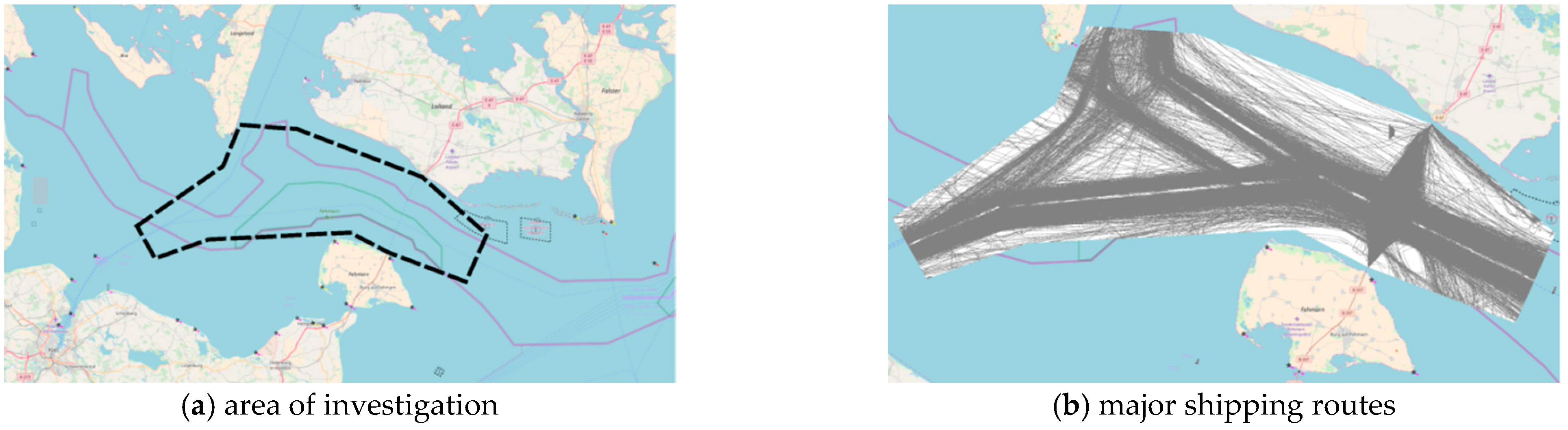
2.1. Database

For the intended simulation study, we focused on close encounters between vessels on the factual traffic data to reflect the reality as close as possible. Currently, the best source of data suitable for tracking vessels’ movements is the automatic identification system (AIS). The AIS data used for this analysis were obtained from the German Waterways and Shipping Administration (WSV). The full dataset covers the period of March 2016. To reflect the specifics of unconstrained waters, the AIS data were spatially extracted for a single region of interest. It contained the vicinity of the Strait of Fehmarn, which is a much-frequented shipping route inbound and outbound of the Baltic Sea and crossed by a busy ferry connection between Puttgarden, Germany, and Rødby, Denmark.

AIS data describing ship movements in constraint waters, such as the Kiel Canal, were excluded from this study, keeping in mind that in constrained waters, close encounters between vessels are unavoidable and happen under controlled conditions. In comparison, in unconstraint waters, close encounters generally have to be avoided for safety reasons. The area of investigation and the major shipping routes obtained from the AIS data within it are shown in Figure 2.

2.2. Incident Detection Method

The AIS data originating from vessels crossing the area of investigation were searched for situations when a pair of vessels reached their closest point of approach (CPA) at a given moment of their voyage. Encounters, whose distance at CPA was more than 6 nautical miles (nm), were excluded from the analysis. If two vessels had multiple close encounters with distances less than 6 nm in the considered area, each such event was accounted for.

2.3. Detected Encounters

Figure 3a depicts the positions of all relevant encounters between vessels in the area of investigation during March 2016.

It is noticeable that a high concentration of close encounters followed the pattern of the major traffic routes within the area of investigation. The routes are defined by two main groups of vessels: those, which use the Kiel Canal, and those, which have to pass Skagen due to their size and draught. A full range of situations, including crossing and overtaking, can be observed, too. Additionally, the ferries connecting Puttgarden, Germany, with Rødby, Denmark, contributed to a high volume of traffic in the Strait of Fehmarn while crossing the busy route inbound and outbound of the Baltic Sea. Figure 3b shows the histogram of the smallest distances between pairs of vessels during their encounters. An increased frequency is seen at three distances: 0.3 nm (1.3% of all encounters), 0.8 nm (2%), and 2.7 nm (2.5%).

The location of encounters, which occurred at distances of about 0.3 nm, are shown in Figure 4a. It can be noticed that there were two main routes within the area of investigation, on which vessels approached each other at the distance of 0.3 nm. First, the vessels operating between Kiel and the Baltic Sea tended to overtake one another with such a narrow berth. Second, the ferries commuting between Puttgarden and Rødby seemingly often passed one another at about 0.3 nm. There were always two ferries inbound to Germany and the other two ferries outbound to Denmark at the same time, probably due to the ferry schedules. They passed one another at three characteristic points of their voyage—at the harbour approaches and halfway between the two ports.

Figure 4b depicts the positions of encounters, which occurred at a distance of about 0.8 nm. It can be observed that the majority of vessels passing one another at the closest distance of 0.8 nm were en route between Kiel Bay and Street of Fehmarn, either inbound or outbound of the Kiel Canal. Those passing situations were complemented by the crossing encounters between the merchant vessels and the Puttgarden–Rødby ferries in the area northeast of the Fehmarn island.

The positions of encounters, which occurred at a distance of about 2.7 nm, are shown in Figure 4c. It should be noted that the encounter distance of 2.7 nm between vessels within the investigation area corresponded mostly to the layout of the recommended routes in the Strait of Fehmarn. The spatial separation between the safe water route to Skagen and the one from Skagen is a good example. Due to the fact that vessels stayed close to the recommended route centreline, the closest points of approach at 2.7 nm are less related to the need for collision avoidance actions and reflect more the regular traffic behaviour.

3. Methodology

3.1. Background

In the seventies, the first ship domains were developed to model the space, which a navigator intends to keep free of obstacles to avoid collisions [14,15]. In the following years, work was carried out on improved modelling to enable the use of the ship domain approach for collision avoidance even in narrow channels, port approach areas, and ports, as well as in specific traffic situations [1,2,16,17,18,22]. Other studies dealt with the application and adaptation of ship domains, either to assess collision risks in specific traffic areas or to support bridge teams in identifying and reducing collision risks [33,34,35]. As a result, it appears reasonable to derive performance requirements for navigation-relevant data from ship-domain-based considerations of collision avoidance emerged [13].

The study in this work assumed that existing collision risks could be mitigated if they were detected early and reliably enough to execute successful evasive manoeuvers as regulated and required (see Figure 5). This means an existing collision risk at the time t_cp can be resolved if its detection at t_cp-δt provides the necessary time span t for the successful implementation of necessary actions, including evasive manoeuvers. Consequently, accuracy requirements for navigation data can be derived by determining under which inaccuracies existing collision risks are not or only incorrectly detected at time point t_cp-δt.

3.2. Modelling

Simulations, as well as theoretical considerations performed for this study, followed the approach presented in [13]. The starting point was a fictitious accident at time t_cp, which takes place in the origin of an accident-centered coordinate system as a fictitious collision point (see Figure 5). Dynamic ship data, such as COG and SOG, were used to determine the position of the two colliding ships A and B at time t_SA = t_cp-δt, where t_SA represents the time at which the decisive situation assessment for the specific accident scenario was performed. The true values of position, COG and SOG were falsified with normally distributed errors for both ships and represented the actual navigational data used for situation assessment at t_SA.

Figure 6 depicts three scenarios for the accuracy of the forecasting of a collision. In Scenario I, the existing collision risk was predicted correctly in time and space, i.e., in or nearby the origin of the coordinate system, because the inaccuracies of the navigational data were small enough. As can be seen in Scenario II, increasing inaccuracies can lead to a non-negligible shift in time and space of the detected collision risk compared to the considered fictitious collision. This implicates that errors in the nautical data lead to an incorrect assessment of the situation and consequently to suboptimal evasive manoeuvers. Finally, Scenario III highlights that extremely large inaccuracies can result in not detecting collision risks because the predicted closest point of approach (CPA), as well as the distance D_CPA of both at this point wrongly indicated a safe passage. As a result, no evasive manoeuvers were initiated, and the collision of both ships became unavoidable.

3.3. Mathematical Formulation

In general, the risk of collision is assessed by estimating the CPA at which the distance D_A,B between both ships A and B reaches its minimum. That means, the CPA is characterised by the minimum distance D_CPA = min(D_A,B) and the remaining time until the CPA occurs, defined as the time to closest point of approach T_CPA.

It is generally known that the CPA parameters can be derived from the relative positions and movements of both ships, as illustrated in Figure 7 [36,37,38,39,40]. P_A and P_B indicate the positions of ships A and B, employing the corresponding x and y coordinates, at the time when situation awareness is performed:

$${\underset{\_}{\mathrm{P}}}_{\mathrm{A}}=\left[\begin{array}{c}{\mathrm{x}}_{\mathrm{A},0}\\ {\mathrm{y}}_{\mathrm{A},0}\end{array}\right];\begin{array}{cc}& {\underset{\_}{\mathrm{P}}}_{\mathrm{B}}=\left[\begin{array}{c}{\mathrm{x}}_{\mathrm{B},0}\\ {\mathrm{y}}_{\mathrm{B},0}\end{array}\right]\end{array}.$$

(1)

Furthermore, the movement of ships A and B is characterised by the velocity vectors S_A and S_B, whose magnitude is determined by the respective SOG values (S_A and S_B) and whose direction is defined by the respective COG values (φ_A and φ_Β):

$${\underset{\_}{\mathrm{S}}}_{\mathrm{A}}={\mathrm{S}}_{\mathrm{A}}\left[\begin{array}{c}\sin \left({\mathsf{\phi }}_{\mathrm{A}}\right)\\ \cos \left({\mathsf{\phi }}_{\mathrm{A}}\right)\end{array}\right];\begin{array}{cc}& {\underset{\_}{\mathrm{S}}}_{\mathrm{B}}={\mathrm{S}}_{\mathrm{B}}\left[\begin{array}{c}\sin \left({\mathsf{\phi }}_{\mathrm{B}}\right)\\ \cos \left({\mathsf{\phi }}_{\mathrm{B}}\right)\end{array}\right]\end{array}$$

(2)

Using the formulas of [36], the time to CPA is given by

$${\mathrm{T}}_{\mathrm{C}\mathrm{P}\mathrm{A}}=-\frac{{\mathrm{S}}_{\mathrm{R},\mathrm{x}}^{}\left({\mathrm{x}}_{\mathrm{A},0}^{}-{\mathrm{x}}_{\mathrm{B},0}^{}\right)+{\mathrm{S}}_{\mathrm{R},\mathrm{y}}^{}\left({\mathrm{y}}_{\mathrm{A},0}^{}-{\mathrm{y}}_{\mathrm{B},0}^{}\right)}{{\mathrm{S}}_{\mathrm{R}}^2}$$

(3)

and the distance at CPA is determined as

$${\mathrm{D}}_{\mathrm{C}\mathrm{P}\mathrm{A}}=\left|\frac{{\mathrm{S}}_{\mathrm{R},\mathrm{y}}\left({\mathrm{x}}_{\mathrm{A},0}^{}-{\mathrm{x}}_{\mathrm{B},0}^{}\right)-{\mathrm{S}}_{\mathrm{R},\mathrm{x}}\left({\mathrm{y}}_{\mathrm{A},0}^{}-{\mathrm{y}}_{\mathrm{B},0}^{}\right)}{{\mathrm{S}}_{\mathrm{R}}}\right|,$$

(4)

where S_R is the relative velocity between the ships A and B and defined by:

$${\underset{\_}{\mathrm{S}}}_{\mathrm{R}}=\left[\begin{array}{c}{\mathrm{S}}_{\mathrm{R},\mathrm{x}}\\ {\mathrm{S}}_{\mathrm{R},\mathrm{y}}\end{array}\right]=\left[\begin{array}{c}{\mathrm{S}}_{\mathrm{A}}\sin {\mathsf{\phi }}_{\mathrm{A}}-{\mathrm{S}}_{\mathrm{B}}\sin {\mathsf{\phi }}_{\mathrm{B}}\\ {\mathrm{S}}_{\mathrm{A}}\cos {\mathsf{\phi }}_{\mathrm{A}}-{\mathrm{S}}_{\mathrm{B}}\cos {\mathsf{\phi }}_{\mathrm{B}}\end{array}\right]={\mathrm{S}}_{\mathrm{R}}\left[\begin{array}{c}\sin {\mathsf{\phi }}_{\mathrm{R}}\\ \cos {\mathsf{\phi }}_{\mathrm{R}}\end{array}\right]$$

(5)

where φ_A and φ_B indicate the course angles of both ships A and B, while φ_R means the course angle of the relative velocity_. The investigations focused on how inaccuracies of individual nautical data affect the correct recognition of existing collision risks. The assumed ship positions P_A^* and P_B^* at the time of situation awareness are determined as the sum of the true position at the time t = -δt and the position errors δx_A, δy_A, δx_B, and δy_B:

$$\begin{array}{l}{\underset{\_}{\mathrm{P}}}_{\mathrm{A}}{}^{\ast }={\underset{\_}{\mathrm{P}}}_{\mathrm{A}}{}^{}+\left[\begin{array}{c}\mathsf{\delta }{\mathrm{x}}_{\mathrm{A}}\\ \mathsf{\delta }{\mathrm{y}}_{\mathrm{A}}\end{array}\right]=-\mathsf{\delta }\mathrm{t}\cdot \left[\begin{array}{c}{\mathrm{S}}_{\mathrm{A}}\sin {\mathsf{\phi }}_{\mathrm{A}}\\ {\mathrm{S}}_{\mathrm{A}}\cos {\mathsf{\phi }}_{\mathrm{A}}\end{array}\right]+\left[\begin{array}{c}\mathsf{\delta }{\mathrm{x}}_{\mathrm{A}}\\ \mathsf{\delta }{\mathrm{y}}_{\mathrm{A}}\end{array}\right]\\ {\underset{\_}{\mathrm{P}}}_{\mathrm{B}}{}^{\ast }={\underset{\_}{\mathrm{P}}}_{\mathrm{B}}{}^{}+\left[\begin{array}{c}\mathsf{\delta }{\mathrm{x}}_{\mathrm{B}}\\ \mathsf{\delta }{\mathrm{y}}_{\mathrm{B}}\end{array}\right]=-\mathsf{\delta }\mathrm{t}\cdot \left[\begin{array}{c}{\mathrm{S}}_{\mathrm{B}}\sin {\mathsf{\phi }}_{\mathrm{B}}\\ {\mathrm{S}}_{\mathrm{B}}\cos {\mathsf{\phi }}_{\mathrm{B}}\end{array}\right]+\left[\begin{array}{c}\mathsf{\delta }{\mathrm{x}}_{\mathrm{B}}\\ \mathsf{\delta }{\mathrm{y}}_{\mathrm{B}}\end{array}\right]\end{array}$$

(6)

The relative velocity S_R^* distorted by errors of SOG and COG follows from:

$${\underset{\_}{\mathrm{S}}}_{\mathrm{R}}{}^{\ast }=\left[\begin{array}{c}{\mathrm{S}}_{\mathrm{R},\mathrm{x}}{}^{\ast }\\ {\mathrm{S}}_{\mathrm{R},\mathrm{y}}{}^{\ast }\end{array}\right]=\left[\begin{array}{c}\left({\mathrm{S}}_{\mathrm{A}}+\mathsf{\delta }{\mathrm{S}}_{\mathrm{A}}\right)\sin \left({\mathsf{\phi }}_{\mathrm{A}}+\mathsf{\delta }{\mathsf{\phi }}_{\mathrm{A}}\right)-\left({\mathrm{S}}_{\mathrm{B}}+\mathsf{\delta }{\mathrm{S}}_{\mathrm{B}}\right)\sin \left({\mathsf{\phi }}_{\mathrm{B}}+\mathsf{\delta }{\mathsf{\phi }}_{\mathrm{B}}\right)\\ \left({\mathrm{S}}_{\mathrm{A}}+\mathsf{\delta }{\mathrm{S}}_{\mathrm{A}}\right)\cos \left({\mathsf{\phi }}_{\mathrm{A}}+\mathsf{\delta }{\mathsf{\phi }}_{\mathrm{A}}\right)-\left({\mathrm{S}}_{\mathrm{B}}+\mathsf{\delta }{\mathrm{S}}_{\mathrm{B}}\right)\cos \left({\mathsf{\phi }}_{\mathrm{B}}+\mathsf{\delta }{\mathsf{\phi }}_{\mathrm{B}}\right)\end{array}\right]={\mathrm{S}}_{\mathrm{R}}{}^{\ast }\left[\begin{array}{c}\sin {\mathsf{\phi }}_{\mathrm{R}}{}^{\ast }\\ \cos {\mathsf{\phi }}_{\mathrm{R}}{}^{\ast }\end{array}\right].$$

(7)

A distortion of ship positions and/or relative ship motion implies that the resulting D_CPA and T_CPA values differ from their correct, true values.

4. Study Results

4.1. Conditions for Critical Misinterpretation

A critical misinterpretation of the current situation occurs when an existing collision risk cannot be detected. This case occurs if D_CPA never becomes smaller than the specified diameter L of an assumed circular ship domain. The resulting conditions are specified in Table 1 for the sole occurrence of different errors based on the mathematical formulation introduced in Section 3.3.

Table 1. Conditions at which individual errors may result in dangerous misinterpretation of an existing collision risk.

(a) Position error only
$$\left|\cos {\mathsf{\phi }}_{\mathrm{R}}\left(\mathsf{\delta }{\mathrm{x}}_{\mathrm{A}}-\mathsf{\delta }{\mathrm{x}}_{\mathrm{B}}\right)-\sin {\mathsf{\phi }}_{\mathrm{R}}\left(\mathsf{\delta }{\mathrm{y}}_{\mathrm{A}}-\mathsf{\delta }{\mathrm{y}}_{\mathrm{B}}\right)\right|\ge \mathrm{L}$$ (8)
(b) SOG error only
$$\left|\frac{\left({\mathrm{S}}_{\mathrm{A}}^{}\mathsf{\delta }{\mathrm{S}}_{\mathrm{B}}^{}-{\mathrm{S}}_{\mathrm{B}}^{}\mathsf{\delta }{\mathrm{S}}_{\mathrm{A}}^{}\right)\sin \left({\mathsf{\phi }}_{\mathrm{A}}^{}-{\mathsf{\phi }}_{\mathrm{B}}^{}\right)}{\sqrt{{\left({\mathrm{S}}_{\mathrm{A}}^{}+\mathsf{\delta }{\mathrm{S}}_{\mathrm{A}}^{}\right)}^2+{\left({\mathrm{S}}_{\mathrm{B}}^{}+\mathsf{\delta }{\mathrm{S}}_{\mathrm{B}}^{}\right)}^2-2\left({\mathrm{S}}_{\mathrm{A}}^{}+\mathsf{\delta }{\mathrm{S}}_{\mathrm{A}}^{}\right)\left({\mathrm{S}}_{\mathrm{B}}^{}+\mathsf{\delta }{\mathrm{S}}_{\mathrm{B}}^{}\right)\cos \left({\mathsf{\phi }}_{\mathrm{A}}^{}-{\mathsf{\phi }}_{\mathrm{B}}^{}\right)}}\right|\cdot \mathsf{\delta }\mathrm{t}\ge \mathrm{L}$$ (9)
(c) COG error only
$$\left|\frac{{\mathrm{S}}_{\mathrm{A}}{}^2\sin \left(\mathsf{\delta }{\mathsf{\phi }}_{\mathrm{A}}\right)+{\mathrm{S}}_{\mathrm{B}}{}^2\sin \left(\mathsf{\delta }{\mathsf{\phi }}_{\mathrm{B}}\right)-2{\mathrm{S}}_{\mathrm{A}}{\mathrm{S}}_{\mathrm{B}}\sin \left(\frac{\mathsf{\delta }{\mathsf{\phi }}_{\mathrm{A}}+\mathsf{\delta }{\mathsf{\phi }}_{\mathrm{B}}}{2}\right)\cos \left({\mathsf{\phi }}_{\mathrm{A}}^{}-{\mathsf{\phi }}_{\mathrm{B}}^{}+\frac{\mathsf{\delta }{\mathsf{\varphi }}_{\mathrm{A}}-\mathsf{\delta }{\mathsf{\varphi }}_{\mathrm{B}}}{2}\right)}{\sqrt{{\mathrm{S}}_{\mathrm{A}}^{}{}^2+{\mathrm{S}}_{\mathrm{B}}^{}{}^2-2{\mathrm{S}}_{\mathrm{A}}^{}{\mathrm{S}}_{\mathrm{B}}^{}\cos \left({\mathsf{\phi }}_{\mathrm{A}}^{}-{\mathsf{\phi }}_{\mathrm{B}}^{}+\mathsf{\delta }{\mathsf{\phi }}_{\mathrm{A}}^{}-\mathsf{\delta }{\mathsf{\phi }}_{\mathrm{B}}^{}\right)}}\right|\cdot \mathsf{\delta }\mathrm{t}\ge \mathrm{L}$$ (10)

Table 1. Conditions at which individual errors may result in dangerous misinterpretation of an existing collision risk.

(a) Position error only
$$\left|\cos {\mathsf{\phi }}_{\mathrm{R}}\left(\mathsf{\delta }{\mathrm{x}}_{\mathrm{A}}-\mathsf{\delta }{\mathrm{x}}_{\mathrm{B}}\right)-\sin {\mathsf{\phi }}_{\mathrm{R}}\left(\mathsf{\delta }{\mathrm{y}}_{\mathrm{A}}-\mathsf{\delta }{\mathrm{y}}_{\mathrm{B}}\right)\right|\ge \mathrm{L}$$ (8)
(b) SOG error only
$$\left|\frac{\left({\mathrm{S}}_{\mathrm{A}}^{}\mathsf{\delta }{\mathrm{S}}_{\mathrm{B}}^{}-{\mathrm{S}}_{\mathrm{B}}^{}\mathsf{\delta }{\mathrm{S}}_{\mathrm{A}}^{}\right)\sin \left({\mathsf{\phi }}_{\mathrm{A}}^{}-{\mathsf{\phi }}_{\mathrm{B}}^{}\right)}{\sqrt{{\left({\mathrm{S}}_{\mathrm{A}}^{}+\mathsf{\delta }{\mathrm{S}}_{\mathrm{A}}^{}\right)}^2+{\left({\mathrm{S}}_{\mathrm{B}}^{}+\mathsf{\delta }{\mathrm{S}}_{\mathrm{B}}^{}\right)}^2-2\left({\mathrm{S}}_{\mathrm{A}}^{}+\mathsf{\delta }{\mathrm{S}}_{\mathrm{A}}^{}\right)\left({\mathrm{S}}_{\mathrm{B}}^{}+\mathsf{\delta }{\mathrm{S}}_{\mathrm{B}}^{}\right)\cos \left({\mathsf{\phi }}_{\mathrm{A}}^{}-{\mathsf{\phi }}_{\mathrm{B}}^{}\right)}}\right|\cdot \mathsf{\delta }\mathrm{t}\ge \mathrm{L}$$ (9)
(c) COG error only
$$\left|\frac{{\mathrm{S}}_{\mathrm{A}}{}^2\sin \left(\mathsf{\delta }{\mathsf{\phi }}_{\mathrm{A}}\right)+{\mathrm{S}}_{\mathrm{B}}{}^2\sin \left(\mathsf{\delta }{\mathsf{\phi }}_{\mathrm{B}}\right)-2{\mathrm{S}}_{\mathrm{A}}{\mathrm{S}}_{\mathrm{B}}\sin \left(\frac{\mathsf{\delta }{\mathsf{\phi }}_{\mathrm{A}}+\mathsf{\delta }{\mathsf{\phi }}_{\mathrm{B}}}{2}\right)\cos \left({\mathsf{\phi }}_{\mathrm{A}}^{}-{\mathsf{\phi }}_{\mathrm{B}}^{}+\frac{\mathsf{\delta }{\mathsf{\varphi }}_{\mathrm{A}}-\mathsf{\delta }{\mathsf{\varphi }}_{\mathrm{B}}}{2}\right)}{\sqrt{{\mathrm{S}}_{\mathrm{A}}^{}{}^2+{\mathrm{S}}_{\mathrm{B}}^{}{}^2-2{\mathrm{S}}_{\mathrm{A}}^{}{\mathrm{S}}_{\mathrm{B}}^{}\cos \left({\mathsf{\phi }}_{\mathrm{A}}^{}-{\mathsf{\phi }}_{\mathrm{B}}^{}+\mathsf{\delta }{\mathsf{\phi }}_{\mathrm{A}}^{}-\mathsf{\delta }{\mathsf{\phi }}_{\mathrm{B}}^{}\right)}}\right|\cdot \mathsf{\delta }\mathrm{t}\ge \mathrm{L}$$ (10)

4.2. Position Error

In Equation (8), the sole occurrence of position errors is considered. In this case, the probability of undetected existing collision risks is only indirectly co-determined by SOG and COG because both specify the course angle of the relative velocity. A north- or southward directed relative velocity (with φ_R~n^.π, integer n) leads to a situation in which the x-component of the relative position error decides primarily on whether an existing collision risk is detected or not. The same is valid for the y-component of the relative positions error if the relative velocity (with φ_R~(n + 0.5)^.π, integer n) is oriented east- or westward. In both cases, an existing collision risk is not detected if the amount of x- or y-components exceeds L. It should be mentioned that other course angles φ_R of the relative velocity are determined by the relative error in the x and y components. If the relative position error is described in polar coordinates, Equation (8) can be transformed as follows:

$$\left|\mathsf{\delta }{\mathrm{r}}_{\mathrm{A},\mathrm{B}}\cdot \sin \left(\mathsf{\delta }{\mathsf{\phi }}_{\mathrm{A},\mathrm{B}}-{\mathsf{\phi }}_{\mathrm{R}}\right)\right|\ge \mathrm{L}$$

(11)

where δr_A,B denotes the absolute value of the relative position error and δφ_A,B means its direction angle. Consequently, if the direction angle δφ_A,B of the relative position error is almost identical to the course angle δφ_R of the relative velocity, it becomes increasingly unlikely that an existing collision risk cannot be detected. This angular dependence can be used to evaluate and display the probability of not recognizing collision risks dependent on the traffic situation, i.e., relative distance and speeds, and the confidence of the position information. From a statistical point of view, however, the course of the relative velocity has no influence on the overall probability that existing collision risks will not be detected. This applies to the case when the position errors of the x and y components follow an average-free normal distribution with standard deviations σ_x and σ_y as assumed for this study. If the errors of the x and y components are assumed to be uncorrelated, then the probability density of position error is:

$$\mathrm{f}\left(\mathsf{\delta }\mathrm{x},\mathsf{\delta }\mathrm{y}\right)=\frac{1}{2\mathsf{\pi }{\mathsf{\sigma }}^2}\exp \left[-\frac{1}{2}\left(\frac{\mathsf{\delta }{\mathrm{x}}^2+\mathsf{\delta }{\mathrm{y}}^2}{{\mathsf{\sigma }}^2}\right)\right]\begin{array}{ccc}& \mathrm{w}\mathrm{i}\mathrm{t}\mathrm{h}& {\mathsf{\sigma }}_{\mathrm{x}}={\mathsf{\sigma }}_{\mathrm{y}}=\mathsf{\sigma }\end{array}.$$

(12)

This implies that the angle difference δφ_A,B-φ_R is equally distributed and, therefore, no longer has statistical relevance.

Figure 8 depicts for exemplary ship domains diameters the probability of not detecting an existing collision risk dependent on the standard deviations of σx and σy using Equation (12). The obtained results indicate that the position errors follow the same curve regardless of the used forecast time t and the ship positions at the time of performed collision risk assessment. The curve (L = 100 m) shows an almost identical behaviour of the curve determined in [13] with the help of synthetically generated AIS data. The probability of scenario III, i.e., the occurrence of an undetected collision risk, follows directly from Equation (12) and is given by:

$$\mathrm{Pr}({\mathrm{S}}_{\mathrm{I}\mathrm{I}\mathrm{I}})=\mathrm{e}\mathrm{r}\mathrm{f}\mathrm{c}(\mathrm{L}/2\cdot \mathsf{\sigma }),$$

(13)

where Pr(^.) denotes the probability of an event and erfc(^.) means the complementary error function.

This result coincided well with the curves shown in Figure 8. Equation (13) illustrates that with an increasing standard deviation of the position error, the probability that existing collision risks are not recognised as such increased. One should note that the size of the ship’s domain, which is the basis on which the collision risk is assessed, also determines the non-detectability of collision risks. It follows that the larger the diameter of the ship domain, the lower the sensitivity to increasing position errors.

4.3. SOG Inaccuracies

Equation9 illustrates the extent to which inaccuracies in SOG measurements can lead to existing collision risks not being detected. It follows that the CPA depends on ships’ course difference φ_A-φ_B, the forecast time δt, as well as the SOG values S_A and S_B and their associated measuring errors δS_A and δS_B. The CPA is influenced by the relative ships’ motion—both real and estimated—but not by the mapping of this into the traffic space. The CPA is also directly proportional to δt. Hence, it becomes unlikely that the collision point will not be detected as such as temporal and spatial proximity increase. On the other hand, detecting collision risks as early as possible ensures that sufficient time is available to resolve the critical situation by appropriate evasive manoeuvers.

Figure 9 shows the effect of SOG inaccuracies on the non-detectability of collision risks P(S_III) dependent on COG differences between both ships. During the simulations on which Figure 9 is based, it was assumed that the SOG inaccuracies of both ships followed the same error distribution, while the ships’ SOG was uniformly distributed between 0 and 25 kn. This explains why the curves showed identical behaviour when the product of forecast time and standard deviation of the SOG inaccuracy was equal. Furthermore, the plots prove the analytical result that an increase in δt at comparable speed inaccuracies leads to an increase in Pr(S_III). It can clearly be seen that Pr(S_III) also increased with increasing standard deviation of the SOG inaccuracies. Pr(S_III) can be greater than 10% if the product of forecast time and SOG standard deviation is higher than 55 m (0.10 kn with 18 min or 0.30 kn with 6 min) and the shipping routes intersect at angles of 40 to 80 degrees. It can be expected that Pr(S_III) changes if the standard deviations of the normally distributed SOG inaccuracies of both ships are different.

Figure 10 shows P(S_III) at (φ_A-φ_B = + π/4) normalised to its maximum of 37.7%. It can be seen that Pr(S_III) is mirror-symmetrical to the line given by σ(δS_A) = σ(δS_B). Furthermore, Pr(S_III) at the point [σ(δS_A) = σ(δS_B) = σ_S] represents the worst case for all SOG inaccuracies with smaller standard deviations, e.g., σ(δS_A) <σ_S or σ(δS_B) <σ_S.

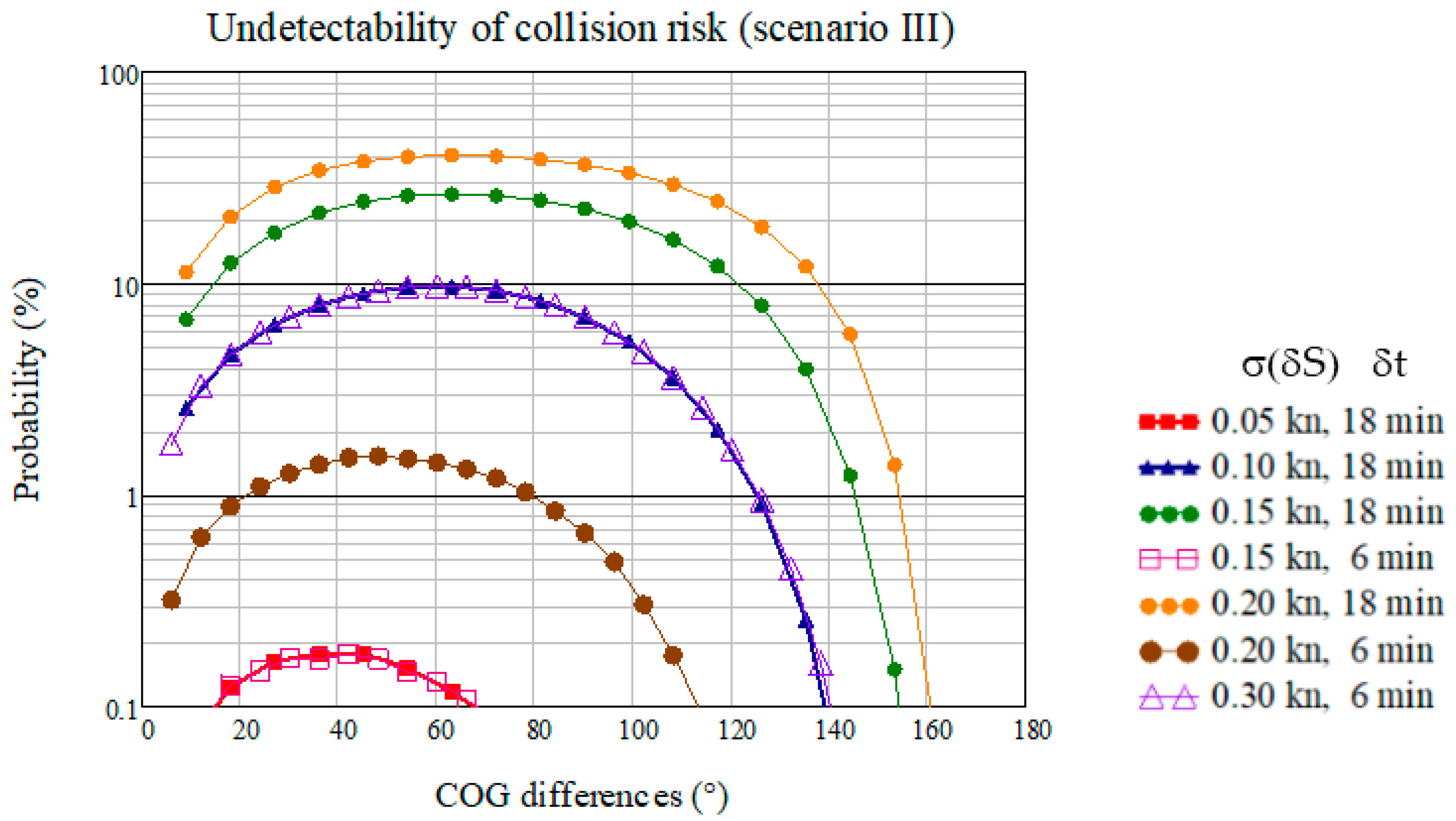
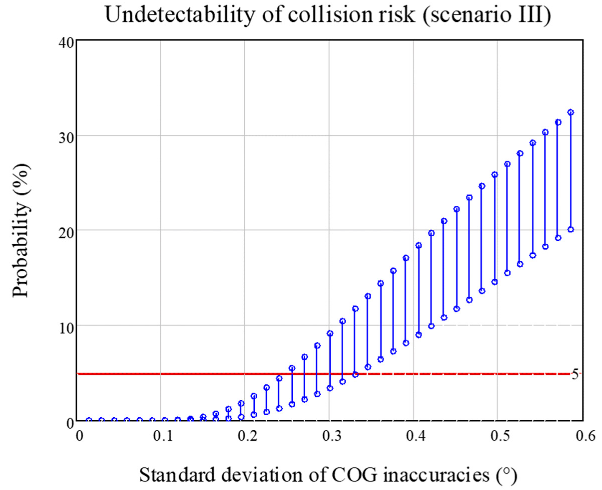
4.4. COG Inaccuracies

The impact of inaccuracies in COG measurements on existing collision risks not being detected is given by Equation (10) and illustrated in Figure 11.

The estimated CPA is determined by the ships’ course difference φ_A-φ_B, the measuring errors δφ_A and δφ_B, the forecast time δt, as well as the SOG values S_A and S_B. It applies here as well that the estimate of CPA is determined by the relative ships’ motion, but not by its mapping into the traffic space. Figure 11 shows the effect of exemplarily selected COG inaccuracies on the detectability of collision risks dependent on occurred COG differences between both ships. During the simulations on which Figure 11 is based, it was assumed that the COG inaccuracies of both ships followed the same error distribution, whereby ships’ SOG was uniformly distributed between 0 and 25 kn. As expected, Pr(S_III) increased with growing forecast time δt. Consequently, Pr(S_III) decreased also with increasing proximity to the real collision point.

It is more surprising that curves showed identical behaviour when the product of forecast time and standard deviation of the COG inaccuracy was equal (0.15° and 18 min vs. 0.45° and 6 min). However, this can be explained by the fact that the following approximation holds for small angles α:

$$\sin \left(\alpha \right)~\alpha \begin{array}{ccc}& \mathrm{w}\mathrm{i}\mathrm{t}\mathrm{h}& \alpha <<1\end{array}.$$

(14)

A standard deviation for COG errors of 0.15° implicates that the value range of COG inaccuracies was limited to (−0.5°, +0.5°), assuming a mean-free normal distribution of COG inaccuracies. If the standard deviation was 0.45°, the value range was well described by (−1.5°, +1.5°), respectively. The residual error of approximation did not exceed 3·10⁻⁶ for a COG inaccuracy of 1.5°. This explains why D_CPA increased proportionally with time as well as proportionally with the standard deviation of the COG inaccuracies.

Figure 11 shows that the highest probability of not detecting existing collision risks is achieved in ship encounters where the ships follow the same COG (φ_A = φ_B) or opposite COG (φ_A = φ_B + π). Of course, this is only true if the behaviour of the COG inaccuracies follows the same distribution function. Consequently, it was justified to make a worst-case estimation for the influence of COG inaccuracies on the non-detectability of collision risks with (φ_A-φ_B = 0) or (φ_A-φ_B = +π).

Figure 12 provides the value range of Pr(S_III) dependent on COG inaccuracies. If Pr(S_III) remains below 5 %, the standard deviation of COG inaccuracies should be below 0.32. This corresponds approximately to the requirement that the error in the COG measurement values must remain below 1°.

4.5. Combination of SOG and COG Inaccuracies

If COG and SOG measurements are inaccurate, P(S_III) is described by Equation (15). The estimated CPA is determined by the ships’ course difference φ_A-φ_B, the measuring errors δφ_A, δφ_B, δS_A and δS_B, the forecast time δt, as well as the SOG values S_A and S_B.

$$\begin{array}{c}\left|\left[\begin{array}{l}\left({\mathrm{S}}_{\mathrm{A}}+\mathsf{\delta }{\mathrm{S}}_{\mathrm{A}}\right)\cdot \sin \left(\mathsf{\delta }{\mathsf{\phi }}_{\mathrm{A}}\right)\cdot \left[{\mathrm{S}}_{\mathrm{A}}-{\mathrm{S}}_{\mathrm{B}}\mathrm{c}\mathrm{o}\mathrm{s}\left({\mathsf{\phi }}_{\mathrm{A}}-{\mathsf{\phi }}_{\mathrm{B}}\right)\right]+\\ \left({\mathrm{S}}_{\mathrm{B}}+\mathsf{\delta }{\mathrm{S}}_{\mathrm{B}}\right)\cdot \sin \left(\mathsf{\delta }{\mathsf{\phi }}_{\mathrm{B}}\right)\cdot \left[{\mathrm{S}}_{\mathrm{B}}-{\mathrm{S}}_{\mathrm{A}}\mathrm{c}\mathrm{o}\mathrm{s}\left({\mathsf{\phi }}_{\mathrm{A}}-{\mathsf{\phi }}_{\mathrm{B}}\right)\right]+\\ \left[{\mathrm{S}}_{\mathrm{A}}\left({\mathrm{S}}_{\mathrm{B}}+\mathsf{\delta }{\mathrm{S}}_{\mathrm{B}}\right)\cos \left(\mathsf{\delta }{\mathsf{\phi }}_{\mathrm{B}}\right)-{\mathrm{S}}_{\mathrm{B}}\left({\mathrm{S}}_{\mathrm{A}}+\mathsf{\delta }{\mathrm{S}}_{\mathrm{A}}\right)\cos \left(\mathsf{\delta }{\mathsf{\phi }}_{\mathrm{A}}\right)\right]\cdot \sin \left({\mathsf{\phi }}_{\mathrm{A}}-{\mathsf{\phi }}_{\mathrm{B}}\right)\end{array}\right]\cdot \frac{\mathsf{\delta }\mathrm{t}}{{\mathrm{S}}_{\mathrm{R}}{}^{\ast }}\right|\ge \mathrm{L}\\ \mathrm{where}\hfill \\ \begin{array}{cc}& {\mathrm{S}}_{\mathrm{R}}{}^{\ast }\end{array}=\sqrt{{\left({\mathrm{S}}_{\mathrm{A}}+\mathsf{\delta }{\mathrm{S}}_{\mathrm{A}}\right)}^2+{\left({\mathrm{S}}_{\mathrm{B}}+\mathsf{\delta }{\mathrm{S}}_{\mathrm{B}}\right)}^2-2\left({\mathrm{S}}_{\mathrm{A}}+\mathsf{\delta }{\mathrm{S}}_{\mathrm{A}}\right)\left({\mathrm{S}}_{\mathrm{B}}+\mathsf{\delta }{\mathrm{S}}_{\mathrm{B}}\right)\cos \left({\mathsf{\phi }}_{\mathrm{A}}^{}-{\mathsf{\phi }}_{\mathrm{B}}^{}+\mathsf{\delta }{\mathsf{\phi }}_{\mathrm{A}}^{}-\mathsf{\delta }{\mathsf{\phi }}_{\mathrm{B}}^{}\right)}\end{array}$$

(15)

Figure 13 indicates that SOG inaccuracies with a standard deviation of 0.065 kn led to a non-detection of existing accident risks in slightly more than 1% of all cases (pink curve) if position and COG were assumed as error-free. If only COG inaccuracies occurred, the standard deviation of COG errors must not be higher than 0.175° to avoid that the probability of non-detection exceeds 1% (orange curve). If COG and SOG were both erroneously measured, Pr(S_III) was almost tripled if the course difference of both vessels is around ±70° (blue curve). The other curves illustrate that a significant reduction in the standard deviation of an error—in the example COG (brown curve) or SOG (black curve) to 20% of its original value—caused the probability curve to approach the curve of single error results.

Table 2. Maximum probability of non-detection of existing collision risks for selected standard deviations of SOG and COG inaccuracies (L = 100 m, SOG uniformly distributed between 0 and 25 kn).

δCOG (°)		0.1			0.2
	δSOG (kn)	0.05	0.10	0.15	0.01	0.05	0.10	0.15
δt (min)
18		0.4	10.8	27.4	2.1	2.30	13.6	29.2
12		0.0	1.8	10.2	0.16	0.17	2.70	11.6
6		0.0	0.0	0.20	0.0	0.0	0.0	0.26

provides the maximum probability of non-detection of existing collision risks for selected SOG and COG inaccuracies. Again, increased standard deviations of SOG and COG inaccuracies, as well as longer prediction times, have a negative impact on the detection probability of collision risks.

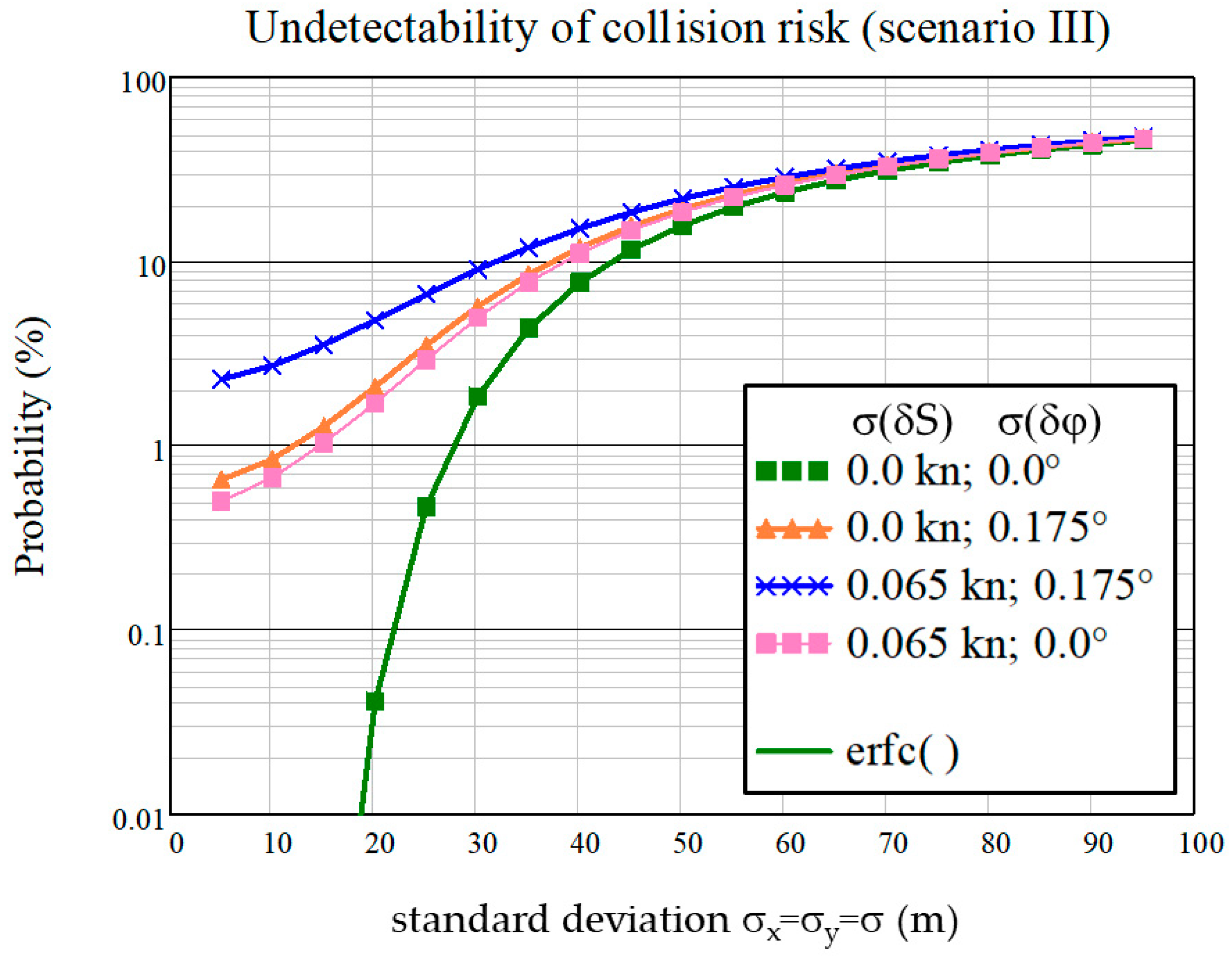
4.6. Position, SOG and COG Inaccuracies

Under real conditions, inaccuracies of position, COG and SOG values will occur at the same time. In this case, the condition defined in Equation (15) has to be extended by an additive term, which results from the considered position error:

$$\begin{array}{c}\left|\left[\begin{array}{l}\left({\mathrm{S}}_{\mathrm{A}}+\mathsf{\delta }{\mathrm{S}}_{\mathrm{A}}\right)\cdot \sin \left(\mathsf{\delta }{\mathsf{\phi }}_{\mathrm{A}}\right)\cdot \left[{\mathrm{S}}_{\mathrm{A}}-{\mathrm{S}}_{\mathrm{B}}\mathrm{c}\mathrm{o}\mathrm{s}\left({\mathsf{\phi }}_{\mathrm{A}}-{\mathsf{\phi }}_{\mathrm{B}}\right)\right]+\\ \left({\mathrm{S}}_{\mathrm{B}}+\mathsf{\delta }{\mathrm{S}}_{\mathrm{B}}\right)\cdot \sin \left(\mathsf{\delta }{\mathsf{\phi }}_{\mathrm{B}}\right)\cdot \left[{\mathrm{S}}_{\mathrm{B}}-{\mathrm{S}}_{\mathrm{A}}\mathrm{c}\mathrm{o}\mathrm{s}\left({\mathsf{\phi }}_{\mathrm{A}}-{\mathsf{\phi }}_{\mathrm{B}}\right)\right]+\\ \left[{\mathrm{S}}_{\mathrm{A}}\left({\mathrm{S}}_{\mathrm{B}}+\mathsf{\delta }{\mathrm{S}}_{\mathrm{B}}\right)\cos \left(\mathsf{\delta }{\mathsf{\phi }}_{\mathrm{B}}\right)-{\mathrm{S}}_{\mathrm{B}}\left({\mathrm{S}}_{\mathrm{A}}+\mathsf{\delta }{\mathrm{S}}_{\mathrm{A}}\right)\cos \left(\mathsf{\delta }{\mathsf{\phi }}_{\mathrm{A}}\right)\right]\cdot \sin \left({\mathsf{\phi }}_{\mathrm{A}}-{\mathsf{\phi }}_{\mathrm{B}}\right)\end{array}\right]\cdot \frac{\mathsf{\delta }\mathrm{t}}{{\mathrm{S}}_{\mathrm{R}}{}^{\ast }}+\Delta {\mathrm{D}}_{\mathrm{C}\mathrm{P}\mathrm{A}}\right|\ge \mathrm{L}\\ \mathrm{where}\hfill \\ \Delta {\mathrm{D}}_{\mathrm{C}\mathrm{P}\mathrm{A}}=\left|\cos {\mathsf{\phi }}_{\mathrm{R}}^{\ast }\left(\mathsf{\delta }{\mathrm{x}}_{\mathrm{A}}-\mathsf{\delta }{\mathrm{x}}_{\mathrm{B}}\right)-\sin {\mathsf{\phi }}_{\mathrm{R}}^{\ast }\left(\mathsf{\delta }{\mathrm{y}}_{\mathrm{A}}-\mathsf{\delta }{\mathrm{y}}_{\mathrm{B}}\right)\right|.\end{array}$$

(16)

The term ΔD_CPA is similar to Equation (8) with the difference that the direction angle of the true relative velocity φ_R is replaced by the one of the estimated relative velocity, i.e., φ_R^*. The standard deviations of the SOG, COG and position inaccuracies determine whether one source of error dominates the probability of non-detection of a collision or all sources of error have a significant impact.

Figure 14 indicates that the probability Pr(S_III) is higher when inaccuracies occur equally in all data used for CPA estimation. This effect has already been observed when COG and SOG are simultaneously subject to errors (see Figure 13). The results depicted in Figure 14 include the results of all course combinations, such that the dependence on ships’ course difference φ_A-φ_B noted in Figure 13 is no longer apparent here. Figure 14 shows that for small position errors (standard deviations of the inaccuracies of the x and y components below 20 m), the SOG and COG inaccuracies dominantly determine the probability Pr(S_III) that existing collision risks cannot be detected. It should be mentioned here that the standard deviations of inaccuracies considered mean that the maximum values of the COG errors were less than 0.7° and the SOG errors were less than 0.14 m/s. This corresponds to typical performance requirements as specified in [32,41].

5. Discussion

In our study, we have shown that inaccurate navigational data may lead to a misevaluation of the current collision risk. More precisely, inaccuracies in navigation-related data can make it impossible to identify an existing collision risk if the navigator relies solely on implemented CPA/TCPA warnings. In these situations, it must be feared that decision-making is not adjusted to the dangerous situation.

The initial results presented in this paper were obtained with a simple simulation setting, which leaves space for further refinement. Certainly, the detection probability will change if the collision risk is assessed using the shape of the ship hull rather than a circular ship domain. The modelling of the inaccuracies as mean-free, normally distributed and uncorrelated may be replaced by a more detailed error model as well. To initialise our simulation setup, we used AIS data collected in and around the Strait of Fehmarn, which we considered a representative traffic area. As the AIS data were only used to extract close encounters between ships, the original quality of the AIS data and the fact that the data had been collected back in 2016 had no effect on the obtained simulation results. In contrast, the study results may help to assess how improved AIS data quality would enhance the detection probability of collision risk. One may note that the study results must not be interpreted as absolute values of the detection probability of collision risks in the considered traffic area as only close ship encounters were extracted from the AIS data, and all other traffic was not incorporated.

Not surprisingly, as the inaccuracies of navigation data increased, so did the probability P(S_III) that existing collision risks would not be detected by the navigational equipment as such. Of more concern is that these situations occurred with non-negligible probability even if position data, COG, and SOG were provided with the accuracy required in the performance standards. For example, the horizontal position error should be in 95% of the cases smaller than 100 m (open sea) or 10 m (coast and port) [42]. For normally distributed mean-free error magnitudes of the x- and y-components of the horizontal position, the standard deviation should be less than 40 m and 4 m, respectively. Assuming that a ship domain’s diameter of 100 m is more applicable to coastal and port areas, the probability P(S_III) is less than 10⁻¹⁰% and thus negligible. However, this value becomes obsolete when the additional influence of SOG and COG inaccuracies is considered. As shown in Figure 14, the non-detection probability can increase to more than 1%, although typical accuracy requirements are over fulfilled with δσ_S < 0.033 m/s and δσ_φ < 0.175°. The prediction time of 18 min used in the simulations was in the order of magnitude often mentioned for the first initial situation assessment of the watch-standing officers and sufficient for successfully initiating and implementing evasive manoeuvers to avoid collisions when needed [5,19]. Routine reassessment of traffic conditions at regular intervals, e.g., every minute, can further reduce the probability P(S_III) but also reduces the scope for actionable measures to address existing collision risks effectively. This illustrates, on the one hand, that other ships with which there is a comparatively low risk of collision must also be assessed on a continuous basis. On the other hand, an integrity assessment of CPA data may help to motivate the navigator to reassess collision risks according to good seamanship and to perform these reassessments with a priority derived from the remaining risk. The latter is gaining importance, especially when humans are less involved, as assessing and correcting element. This will be the case when the automation level of ship navigation increases.

6. Conclusions

The knowledge about the exact own ship’s position and movement is an essential prerequisite for safe ship navigation, supports minimizing fuel consumption, contributes to reducing emissions of greenhouse gases, and ensures on-time delivery of goods. Information about the exact position in relation to the planned track as well as to dangerous depth lines contributes to grounding avoidance as well. Moreover, the exchange of real-time PNT-data between ships via AIS enables calculating encounter parameters and supports the assessment of the collision risk in current and emerging navigational situations by navigators, such as captains, pilots and OOWs. Hence, they exploit the potentials of sophisticated PNT-equipment. At the same time, navigators need to know the capability limits of the navigational systems and have to be well aware that collision risks can also result from incorrect navigational data being used for situation assessment.

How a collision risk assessment should be performed under consideration of the sensors and data sources’ current performance is an open research question. However, the study has proved the relevance of this question and illustrated the need to develop suitable solutions. Moreover, this work, for the very first time, associates collision risk and error margins through a comprehensive and detailed analysis of the impact of PNT-data error limits. The obtained results may complement the existing ARPA performance standards [43].

References

1. Xu, Q.; Wang, N. A Survey on Ship Collision Risk Evaluation. Traffic Transp. 2014, 26, 475–486. [Google Scholar] [CrossRef]
2. Pietrzykowski, Z. Ship’s Fuzzy Domain—A Criterion for Navigational Safety in Narrow Fairways. J. Navig. 2008, 61, 499–514. [Google Scholar] [CrossRef]
3. Goerlandt, F.; Montewka, J.; Lammi, H.; Kujala, P. Analysis of near collisions in the Gulf of Finland. In Advances in Safety, Reliability and Risk Management; CRC Press: Boca Raton, FL, USA, 2011; pp. 2880–2886. [Google Scholar]
4. Johansen, T.A.; Perez, T.; Cristofaro, A. Ship Collision Avoidance and COLREGS Compliance Using Simulation-Based Control Behavior Selection with Predictive Hazard Assessment. IEEE Trans. Intell. Transp. Syst. 2016, 17, 3407–3422. [Google Scholar] [CrossRef] [Green Version]
5. Baldauf, M.; Mehdi, R.; Deeb, H.; Schröder-Hinrichs, J.U.; Benedict, K.; Krüger, C.; Fischer, S.; Gluch, M. Manoeuvring areas to adapt ACAS for the maritime domain. Sci. J. Marit. Univ. Szczec. 2015, 43, 39–47. [Google Scholar] [CrossRef]
6. Baldauf, M.; Benedict, K.; Fischer, S.; Motz, F.; Schröder-Hinrichs, J.-U. Collision avoidance systems in air and maritime traffic. Proc. Inst. Mech. Eng. Part O J. Risk Reliab. 2011, 225, 333–343. [Google Scholar] [CrossRef]
7. Mehdi, R.A.; Baldauf, M.; Deeb, H. A dynamic risk assessment method to address safety of navigation concerns around offshore renewable energy installations. Proc. Inst. Mech. Eng. Part M J. Eng. Marit. Environ. 2020, 234, 231–244. [Google Scholar] [CrossRef]
8. IMO. Report of the Maritime Safety Committee, Strategy for the Development and Implementation of E-Navigation, MSC\85\26, Annex 20; International Maritime Organization: London, UK, 2009. [Google Scholar]
9. IMO. NCSR1 Report to the Maritime Safety Committee: Draft E-Navigation Strategy Implementation Plan. NCSR1/28 Annex 7; International Maritime Organization: London, UK, 2014. [Google Scholar]
10. IMO. Performance Standards for Multi-System Shipborne Radionavigation Receivers. MSC 95/22/Add.2 Annex17; International Maritime Organization: London, UK, 2014. [Google Scholar]
11. IMO. Guidelines for Shipborne Position, Navigation and Timing (Pnt) Data Processing. MSC.1/Circ.1575; International Maritime Organization: London, UK, 2017. [Google Scholar]
12. IMO. Revised Maritime Policy and Requirements for a Future Global Navigation Satellite System (GNSS), Resolution A.915(22); International Maritime Organization: London, UK, 2001. [Google Scholar]
13. Banyś, P.; Engler, E.; Heymann, F. Interdependencies Between Evaluation of Collision Risks and Performance of Shipborne Pnt Data Provision. Transp. Probl. 2017, 11, 151–165. [Google Scholar] [CrossRef] [Green Version]
14. Fujii, Y.; Tanaka, K. Traffic Capacity. J. Navig. 1971, 24, 543–552. [Google Scholar] [CrossRef]
15. Goodwin, E.M. A Statistical Study of Ship Domains. J. Navig. 1975, 28, 328–344. [Google Scholar] [CrossRef] [Green Version]
16. Davis, P.V.; Dove, M.J.; Stockel, C.T. A Computer Simulation of Marine Traffic Using Domains and Arenas. J. Navig. 1980, 33, 215–222. [Google Scholar] [CrossRef]
17. Wang, T.; Yan, X.P.; Wang, Y.; Wu, Q. Ship Domain Model for Multi-ship Collision Avoidance Decision-making with COLREGs Based on Artificial Potential Field. TransNav Int. J. Mar. Navig. Saf. Sea Transp. 2017, 11, 85–92. [Google Scholar] [CrossRef] [Green Version]
18. Ning, W.; Xianyao, M.; Qingyang, X.; Zuwen, W. A Unified Analytical Framework for Ship Domains. J. Navig. 2009, 62, 643–655. [Google Scholar] [CrossRef]
19. Hilgert, H.; Baldauf, M. A common risk model for the assessment of encounter situations on board ships. Dtsch. Hydrogr. Z. 1997, 49, 531–542. [Google Scholar] [CrossRef]
20. Dinh, G.H.; Im, N. The combination of analytical and statistical method to define polygonal ship domain and reflect human experiences in estimating dangerous area. Int. J. e-Navig. Marit. Econ. 2016, 4, 97–108. [Google Scholar] [CrossRef] [Green Version]
21. Szlapczynski, R.; Szlapczynska, J. Review of ship safety domains: Models and applications. Ocean Eng. 2017, 145, 277–289. [Google Scholar] [CrossRef]
22. Szlapczynski, R.; Szlapczynska, J. A method of determining and visualizing safe motion parameters of a ship navigating in restricted waters. Ocean Eng. 2017, 129, 363–373. [Google Scholar] [CrossRef]
23. Szlapczynska, J.; Szlapczynski, R. Heuristic Method of Safe Manoeuvre Selection Based on Collision Threat Parameters Areas. TransNav Int. J. Mar. Navig. Saf. Sea Transp. 2017, 11, 591–596. [Google Scholar] [CrossRef] [Green Version]
24. Szlapczynski, R.; Krata, P.; Szlapczynska, J. Ship domain applied to determining distances for collision avoidance manoeuvres in give-way situations. Ocean Eng. 2018, 165, 43–54. [Google Scholar] [CrossRef]
25. Szlapczynski, R.; Krata, P. Determining and visualizing safe motion parameters of a ship navigating in severe weather conditions. Ocean Eng. 2018, 158, 263–274. [Google Scholar] [CrossRef]
26. Ożoga, B.; Montewka, J. Towards a decision support system for maritime navigation on heavily trafficked basins. Ocean Eng. 2018, 159, 88–97. [Google Scholar] [CrossRef]
27. Kondo, M.; Shoji, R.; Miyake, K.; Zhang, T.; Furuya, T.; Ohshima, K.; Inaishi, M.; Nakagawa, M. The “Watch” Support System for Ship Navigation. In Mining Data for Financial Applications; Springer Nature: London, UK, 2018; Volume 10905, pp. 429–440. [Google Scholar]
28. Gil, M.; Montewka, J.; Krata, P.; Hinz, T.; Hirdaris, S. Determination of the dynamic critical maneuvering area in an encounter between two vessels: Operation with negligible environmental disruption. Ocean Eng. 2020, 213, 107709. [Google Scholar] [CrossRef]
29. Gil, M.; Montewka, J.; Krata, P.; Hinz, T.; Hirdaris, S. Semi-dynamic ship domain in the encounter situation of two vessels. In Developments in the Collision and Grounding of Ships and Offshore Structures; CRC Press: Boca Raton, FL, USA, 2019; pp. 301–307. [Google Scholar]
30. Baldauf, M.; Mehdi, R.; Fischer, S.; Gluch, M. A perfect warning to avoid collisions at sea? Sci. J. Marit. Univ. Szczec. 2017, 49, 53–64. [Google Scholar] [CrossRef]
31. Van Westrenen, F.; Baldauf, M. Improving conflicts detection in maritime traffic: Case studies on the effect of traffic complexity on ship collisions. Proc. Inst. Mech. Eng. Part M: J. Eng. Marit. Environ. 2019, 234, 209–222. [Google Scholar] [CrossRef]
32. IMO. Resolution A.824(19) Performance standards for devices to indicate speed and distance (MSC.96(72)); International Maritime Organization: London, UK, 1997. [Google Scholar]
33. Qu, X.; Meng, Q.; Suyi, L. Ship collision risk assessment for the Singapore Strait. Accid. Anal. Prev. 2011, 43, 2030–2036. [Google Scholar] [CrossRef] [PubMed] [Green Version]
34. Bakdi, A.; Glad, I.; Vanem, E.; Engelhardtsen, Ø. AIS-Based Multiple Vessel Collision and Grounding Risk Identification based on Adaptive Safety Domain. J. Mar. Sci. Eng. 2019, 8, 5. [Google Scholar] [CrossRef] [Green Version]
35. Li, M.; Mou, J.; Liu, R.; Chen, P.; Dong, Z.; He, Y. Relational Model of Accidents and Vessel Traffic Using AIS Data and GIS: A Case Study of the Western Port of Shenzhen City. J. Mar. Sci. Eng. 2019, 7, 163. [Google Scholar] [CrossRef] [Green Version]
36. Lenart, A.S. Manoeuvring to Required Approach Parameters—CPA Distance and Time. In Annual of Navigation; Polish Academy of Sciences, Polish Navigation Forum: Gdynia, Poland, 1999; pp. 99–108. [Google Scholar]
37. Lenart, A.S. Manoeuvring to Required Approach Parameters—Distance and Time on Course. In Annual of Navigation; Polish Academy of Sciences, Polish Navigation Forum: Gdynia, Poland, 1999; pp. 109–115. [Google Scholar]
38. Lenart, A. Approach Parameters in Marine Navigation—Graphical Interpretations. TransNav Int. J. Mar. Navig. Saf. Sea Transp. 2017, 11, 521–529. [Google Scholar] [CrossRef] [Green Version]
39. Szlapczynski, R. A Unified Measure of Collision Risk Derived from the Concept of a Ship Domain. J. Navig. 2006, 59, 477–490. [Google Scholar] [CrossRef]
40. Bole, A.; Wall, A.D.; Norris, A. Radar and ARPA Manual: Radar, AIS and Target Tracking for Marine Radar, 3rd ed.; Butterworth-Heinemann: Oxford, UK, 2014. [Google Scholar]
41. IMO. Resolution A.424(XI), Performance Standards for Gyro-Compasses; International Maritime Organization: London, UK, 1979. [Google Scholar]
42. IMO. Resolution A.1046(27) Worldwide Radionavigation System; International Maritime Organization: London, UK, 2011. [Google Scholar]
43. IMO. Resolution A.823(19), Performance Standards for Automatic Radar Plotting Aids (Arpas); International Maritime Organization: London, UK, 1995. [Google Scholar]
Figure 1. Grade I to IV specify the amount and types of PNT data needed for specific navigational applications and phases, as defined in [32] (CCRP—consistent common reference point, PVT—position, velocity, and time, SOG—speed-over-ground, COG—course-over-ground, STW—speed-through-water, CTW—course-Through-water; * stands for improved accuracy and integrity in comparison to Grade II).
Jmse 09 00149 g001
Figure 2. Database: (a) the polygon defining the area for the automatic identification system (AIS) data analysis and (b) the major shipping routes derived from AIS data.
Jmse 09 00149 g002
Figure 3. Encounters (marked with x) between pairs of vessels closer than 6 nm during March 2016 in the vicinity of Fehmarn: (a) position of encounters and (b) histogram of observed encounter distances.
Jmse 09 00149 g003
Figure 4. The positions of encounters (marked with x) between pairs of vessels at their closest point of approach: separated from each other by (a) 0.3 nm, (b) 0.8 nm, and (c) 2.7 nm.
Jmse 09 00149 g004
Figure 5. Collision point and area of ships A and B if they follow their planned route and continue their movement (tcp = time of collision, δt = time span to prevent collision).
Jmse 09 00149 g005
Figure 6. Impact of position, navigation and timing (PNT) data accuracy on the assessment of collision risk (collision area is marked with a red circle in case A and B; xcp and ycp—coordinates of collision point; DCPA—distance between both ships at the closest point of approach (CPA)).
Jmse 09 00149 g006
Figure 7. Relative data-based representation of ship encounters (the parameters are detailed in the text).
Jmse 09 00149 g007
Figure 8. Undetectability of existing collision risks for exemplary diameters L of ship domains dependent on the assumed standard deviation of position error.
Jmse 09 00149 g008
Figure 9. Impact of speed-over-ground (SOG) inaccuracies on the detectability of existing collision risks dependent on the COG differences φAB between both ships (L = 100 m, provided for selected forecast times δt and standard deviations σ(δSA) = σ(δSB) = σ(δS) of SOG inaccuracies).
Jmse 09 00149 g009
Figure 10. Probability of undetected collisions risks (colour-represented value range between 0 and 37.7%) dependent on the standard deviation of SOG inaccuracies with values between 0 and 0.2 kn (φAB =+π/4; L = 100 m; δt = 18 min).
Jmse 09 00149 g010
Figure 11. Impact of course-over-ground (COG) inaccuracies on the probability of undetected collisions risks dependent on COG differences φAB between both ships (L = 100 m, provided for selected forecast times δt, equally distributed SOG values between 0 and 25 kn and standard deviations σ(δφA) = σ(δφB) = σ(δφ) of COG inaccuracies).
Jmse 09 00149 g011
Figure 12. Range of probabilities of undetected collisions risks dependent on the standard deviation of COG inaccuracies (L = 100 m, provided for a forecast time δt = 6 min and equally distributed SOG values between 0 and 25 kn).
Jmse 09 00149 g012
Figure 13. Impact of COG and SOG inaccuracies on the probability of undetected collisions risks dependent, on occurred COG differences φAB between both ships (L = 100 m, provided for a forecast time δt = 18 min, equally distributed SOG values between 0 and 25 kn, and selected standard deviations σ(δφ) and σ(δS)).
Jmse 09 00149 g013
Figure 14. Impact of position, COG and SOG inaccuracies on the detectability of existing collision risks dependent on the standard deviation σ of position errors (L = 100 m, provided for a forecast time δt = 18 min, equally distributed SOG values between 0 and 25 kn and equally distributed COG values between 0° and 360°).
Jmse 09 00149 g014