Abstract
The prediction of loss of position in the offshore industry would allow optimization of dynamic positioning drilling operations, reducing the number and severity of potential accidents. In this paper, the probability of an excursion is determined by developing binary logistic regression models based on a database of 42 incidents which took place between 2011 and 2015. For each case, variables describing the configuration of the dynamic positioning system, weather conditions, and water depth are considered. We demonstrate that loss of position is significantly more likely to occur when there is a higher usage of generators, and the drilling takes place in shallower waters along with adverse weather conditions; this model has very good results when applied to the sample. The same method is then applied for obtaining a binary regression model for incidents not attributable to human error, showing that it is a function of the percentage of generators in use, wind force, and wave height. Applying these results to the risk management of drilling operations may help focus our attention on the factors that most strongly affect loss of position, thereby improving safety during these operations.
1. Introduction
Despite the efforts of the industry to achieve a high level of safety in the use of dynamic positioning (DP) during drilling operations, there have been some accidents with severe consequences. For example, in March 2006, the Diamond Ocean Confidence, a semi-submersible rig performing drilling operations in the Gulf of Mexico, spilled over 200 barrels of synthetic-based drilling fluid, when the riser emergency disconnection failed after a DP system failure [1,2]. Further, in 2003, the Transocean drillship Discoverer Enterprise was completing a well in the Gulf of Mexico, when the ship lost her position and the riser, 6000 feet in length, was snapped off in two places. In this case, the accident did not have severe consequences as a blowout preventer (BOP) sealed off the well below it and prevented any oil spill [3]. These examples of accidents due to loss of position (LoP) during drilling operations illustrate the importance of achieving and maintaining good station-keeping performance [4] in ensuring the safety of drilling operations.
DP drilling incidents have been the subject of considerable academic research. In 2011, Haibo Chen [5] published a paper characterizing the safety of DP operations based on a barrier model and proposing safety measures to be taken at each stage of the LoP. Previously, the same research team had published an article about the safety of such units [6], considering both LoP and recovery.
A very interesting approach to the human factors in DP incidents was proposed by Chae [7], and the same group demonstrated this approach using Bayesian networks to identify the leading causes of LoP while using DP, analyzing the type of human error leading to losses of position [8]. Dong et al. [9] focused their research on incidents that had taken place during offshore loading operations, applying Man, Technology, and Organization (MTO) analysis for detecting the main causes, which appeared to be a combination of technical, human, and organizational failures. Øvergård et al. [10] also researched the human element during DP incidents, exploring the influence of situational awareness during these operations. Nie et al. [1] applied an innovative approach based on dynamic Bayesian networks and gene ontology to analyze the prediction of drilling riser emergency disconnection in deep water.
Drilling operations take place over a wellhead. Onboard a drilling vessel, the primary function of a DP system on board a drilling vessel, known as the riser angle or follow mode, is to maintain the position of the vessel such that the riser/stack angle, containing the drill string, is close to zero, compensating for currents or tidal flow as necessary [11]. This angle is measured between the riser (on the top) and the wellhead or lower marine riser package (LMRP) [12]. The angle is monitored by the dynamic positioning operator (DPO) through sensors located around the LMRP. A watch circle system is created to help the DPO monitor the movements of the vessel. Under normal conditions, the vessel is operated within the green circle (as shown in Figure 1). In the event of an incident where the system is incapable of maintaining position, there will be an excursion (known as drift-off or drive-off, depending on the cause and movement) beyond the green circle. In this case, the blue (advisory) alarm will be raised, indicating a degrading status.
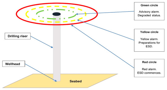
Figure 1.
Dynamic positioning watch circle (the excursion limits are not to scale; ESD: emergency shutdown; created by the authors).
When the excursion continues beyond the yellow circle, the yellow alarm should be raised, and preparations should be made for emergency disconnection. In the event of the excursion continuing beyond the red circle, the red alarm is triggered, a controlled emergency disconnection is initiated [1,5], and the well is shut. Should the vessel pass the physical limit, the riser would break, and the consequences would be catastrophic [13], both economically and environmentally.
Various criteria may be applied to set the limits of the watch circles. Some authors argue that the circles should be based on the riser/stack angle, and specifically, Chen et al. [5] state that the yellow circle should be set at an angle of 3 degrees and the red circle at an angle of 5 degrees. This approach is valid for shallow waters. In deeper waters, as Bray [14] indicates, tidal flow should be taken into account, compensating for its effect on the riser.
On the other hand, several studies in this field [15,16,17,18,19] suggest that there are other factors to be considered (for example, other structures in the vicinity, riser tensioner pulldown, riser connectors, emergency disconnection time frame, among others), on a case-by-case basis. The Marine Technology Society (MTS) supports this idea in its DP Operations Guidance, Part 2, Appendix 1—MODUs [13], where the Well-Specific Operating Guidelines (WSOG) are described.
It is important, in safety terms, to identify the potential hazards associated with given operations and determine the probability of incidents occurring and their possible outcomes and consequences. This approach is commonly known as Quantitative Risk Assessment (QRA) [20]. Over the years, the idea of QRA has been improved by the development of various methodologies. Some examples of these are hazard and operability studies (HAZOPs), Failure Mode and Effect Analysis (FMEA), Fault Tree Analysis (FTA), and Event Tree Analysis (ETA) [21]. Another method which has been extensively used for risk analysis of DP incidents is the Bayesian Network (BN), a graphical model that represents the dependency between variables, using nodes and directed links, making it possible to show conditional probabilities for a set of variables [22]. This technique is widely applied in DP incident analysis; however, the parameters used for quantifying the associated risk generally depend on the best judgment of the person performing the analysis [23].
Thanks to the high level of the protective measures taken to prevent catastrophic consequences, the frequency of accidents in the oil and gas industry can be considered low, and therefore, though data on accidents are published, there is a limited volume of accident data available for analysis. That is why incidents and near misses began to be used for updating risk analysis and management [24,25]. Studies using this approach have been reported by Khakzad [26], Yang [27], and more recently, Arnaldo-Valdes [28], Rebello [29], and Shengli and Yongtu [30].
Precursor data for an incident include all the data that may influence a particular incident. When such a database is analyzed, a specific pattern may be seen that could be used to predict an incident. This is the principle underlying the regression modeling technique used in this paper.
Several publications have appeared in recent years documenting the use of regression modeling for predicting and preventing incidents in the transportation field. In terrestrial transportation, logistic regression modeling has been applied in the detection of traffic incidents [31] and their duration [32]. In air transportation, traditionally connected to the maritime industry in terms of safety, this statistical approach has been used for the prediction of incidents due to human error [33,34]. Nonetheless, to the authors’ knowledge, there are very few publications in the literature that address the use of logistic regression modeling for the prediction of incidents in the maritime industry. In this field, the research has mainly focused on explaining the influence of human error in those incidents, as discussed by Hogenboom et al. [35] and Weng et al. [36], or as part of variable selection for prediction modeling, as applied by Boullosa-Falces et al. [37].
The research team gathered the data from the International Maritime Contractors Association (IMCA) station keeping incidents reported for 2011 to 2015 [38,39,40,41,42]. From all the events included in these reports, we selected those that took place while there were drilling operations in progress and which included information on all the variables studied, 42 in total. The IMCA DP station keeping reports are considered to be the most complete in the industry, in terms not only of the number of reports included but also of the completeness of the information given.
The most common main causes were environmental conditions, these being considered responsible for 13 incidents (31%); followed by thrusters/propulsion faults cited in 10 cases (23.8%) and human errors and power generation faults in six cases (14.3%) each. The rest of the main causes are computer issues and reference faults in three cases (7.1%) each, and electrical faults in one case (2.4%). It is important to mention that, although main causes were established for all the incidents analyzed, a secondary cause was only identified in 13 cases.
Twenty-nine incidents did not suffer any LoP, while 13 cases had an excursion. From those, nine refer to drift-off and four to drive-off excursions. There was one incident reaching the green circle, nine cases surpassing the yellow circle, and in three incidents the vessel reached the red circle.
Since 2016, due to the volume of DP incidents received, only a small sample of the most serious incidents was published by IMCA in DP Event Bulletins [43]. This change in format made the research team consider to only use the period for which all DP incidents were given as event trees.
In this paper, binary logistic regression is applied to obtain a formula that gives the probability of a LoP during DP drilling operations. As the occurrence likelihood of a LoP during drilling operations can be affected by a range of variables at the same time, the main aim was to find a model expressing the quantitative likelihood of a DP incident ending in an excursion during DP drilling operations, that is, obtain a formula that would help determine what characterizes LoP cases. In this way, it is expected that safety procedures could be specified more precisely, helping operators to improve their understanding of the operational environment and ensure safer operations.
The specific objectives proposed are as follows:
- to analyze the variables included in the incident reports and extract data for regression modeling;
- to construct models, using binary logistic regression, predicting the probability of a LoP; and
- to explore whether or not human factors were considered to have contributed to the LoP.
With the model obtained from this research, drilling companies and other authorities would be able to review their management manuals and propose effective measures to reduce the probability of LoP while conducting DP drilling operations. The results obtained by the model reported illustrate the reliability of this approach.
The remainder of this article is organized as follows. Details of the dataset and description of the methods are described in Section 2. Section 3 provides the findings obtained following the implemented methodology. A final evaluation of the findings, including their limitations, is presented in Section 4. Finally, the conclusions obtained are presented in Section 5.
2. Materials and Methods
2.1. Database
The data described in each event tree were carefully read, and a database was developed, including the following variables:
- Water depth (in meters): indicates the water depth at which the drilling operations took place;
- Percentage of thrusters: the number of thrusters online divided by the total number of thrusters, both online and stand-by;
- Percentage of generators: the number of generators online divided by the total number of generators, both online and stand-by;
- DGNSS: the number of Differential Global Navigation Satellite Systems (DGNSS) systems selected in the DP system;
- HPR systems: the number of hydroacoustic position reference (HPR) systems selected in the DP system;
- Taut wires: the number of taut wires in use during the operations;
- Inertia systems: the number of inertia systems in use during the drilling operations;
- Gyros: the number of gyros in use during the drilling operations;
- MRUs: the number of motion reference units (MRUs) in use during the drilling operations;
- Wind sensors: the number of wind sensors in use during the drilling operations;
- Wind force: the force in knots of the wind blowing when the incident occurred;
- Current speed: the speed of the current in knots when the incident occurred;
- Wave height: the height of the waves in meters;
- Visibility: the visibility when the incident happened, categorized as “poor” when the visibility was less than 2 nautical miles, “moderate”, between 2 and 5 nautical miles, and “good”, above 5 nautical miles [44], coded as 1, 2, and 3, respectively;
- Main cause: the leading cause, as given by the IMCA, based on the following categories: Computer, Electrical, Environmental, External, Human error, Power, References, Sensors, and Thruster;
- Secondary cause: the secondary cause, if present, as given by the IMCA, with the same categories as the main cause;
- Excursion: whether or not a LoP occurred (coded as 1 or 0 respectively).
- Human cause: whether or not the main and/or secondary causes are due to human factors (coded as 1 if so, and 0 otherwise).
This database is uploaded to the IBM SPSS Statistics for Windows, version 23.0. Descriptive statistics and correlations among the variables are calculated before developing the binary logistic regression models.
2.2. Binary Logistic Regression Model
Binary logistic regression is a type of regression analysis that can model problems with two possible discrete outcomes. The model obtained can be used to predict the possibilities of two different outcomes for a categorical dependent variable with two values, given a set of independent variables.
As the objectives of this study concern LoP in incidents occurring during DP drilling operations, excursion is considered the dependent variable that can take one of two values: 0 if there was no LoP, and 1 if LoP occurred.
Except for the variables water depth, percentage of thrusters online, percentage of generators online, wind force, current speed, and wave height, which are all quantitative, the independent variables are categorical. Given this, the software manipulates its values internally to produce as many variables as there are categories minus one. For example, for Wind sensors, there are five categories, and the statistical software produces four variables: Windsensors (i), i = 1, 2, 3, 4. These new variables can take two values: 1 indicates the presence of a given quality and 0 its absence.
The model for determining LoP in an incident is given by [45] as
where Z is the linear predictor function to determine the excursion of the incident, X1,…, Xk represent each independent variable, k being the number of independent variables, and B0, B1, …, Bk are the regression coefficients to be estimated.
Z = B1 X1 + … + Bk Xk + B0,
The variables entered into the equation of the model given in (1) are selected by the method: Enter [46]. Although the default option of the statistical software takes into account the p-values associated to enter a variable in the equation, modern statistical approaches [47,48] warn about the use of p-values for establishing cut-off values. It is also known that p-values are highly sensitive to sample size, so with a small sample size we have low statistical power and therefore are prone to not observing a statistical effect in the sample when the statistical effect is in reality present in the population. Therefore, the team will focus on effect sizes (ES) and Confidence Intervals (CI) will be shown, indicating the variables that are having a bigger weight in the system rather than rejecting based on the p-value.
This being said, the authors do not want to simply use a default statistical procedure to assess the relationships as pure data-based inference. It is clear that currents, wind force, and other meteorological variables affect the position of a ship, and it would be strange to remove these variables from the model based on the results of the inference. Therefore, the models will include the weather variables.
This software, considering the values of the independent variables in each incident, calculates the probability of excursion in each case. The probability P of excursion in a specific case is given by [49]
P = 1/(1 + exp(−Z)).
This probability P varies between 0 and 1: the closer to 0 the lower the probability of excursion, and the closer to 1, the higher the probability of excursion. According to the obtained value for P, the case will be classified into one of two groups: no excursion (0), for probabilities of less than 0.5 (in other words, the probabilities of having an excursion are less than 50%, hence this case would be classified as no excursion), and excursion (1), for probabilities of more than 0.5 (when the probabilities of LoP are above 50%).
Having developed the model, we need to evaluate its performance, and this can be done by assessing the goodness of fit. That is, the estimated probability of an incident resulting (or not resulting) in an excursion does not necessarily match the actual outcome. For example, the model may define a case as having a significant likelihood of not ending in a LoP, and yet an actual LoP was recorded. In all these cases, there is an error, calculated as the difference between the observed probability and the estimated probability [49]:
where Pi can take the values 0 or 1, depending on whether the case is classified into the first or second group (no excursion or excursion, respectively).
Ei = Pi observed − Pi estimated,
Assessing goodness of fit involves checking how probable the results obtained for the estimated model are, and this can be done by comparing the number of cases in the second group (excursion = yes) with the expected number should the model be valid. This expected number is the product of the total number of cases in the sample by the estimated probability of belonging to the second group.
For this fit, the −2 log likelihood (−2LL) statistic can be used. Lower −2LL values indicate a better fit. A model is considered to show a good fit when p-value < 0.05. Explained variation (R square) is a performance measure that is often used as a logarithmic scoring rule. In this study, the Cox and Snell and Nagelkerke R square will be used [50]. Furthermore, the Cohen’s kappa analysis is used to determine the agreement between the observed and estimated outcomes of the incidents.
In addition, Z2 can be used to compare the observed probabilities with those estimated from the model [49]:
Z2 = (∑ Ei2)/(Pi estimated (1 − Pi estimated)).
Both statistics follow a chi-square distribution with n-2 degrees of freedom, under the hypothesis that the model fits the observed data. Z2 shows the percentage of the correctly classified cases after the model has been defined, indicating the reliability of the model.
In our context, the higher percentage of correctly classified cases the better the performance of the model in predicting whether a given case is a loss-of-position incident: over 75% can be considered very good and over 90% excellent [46].
Last, we analyzed the relative ratio between the probability of the incidents having an excursion (P) and the probability of the incidents not having an excursion (Q). The probability of not having excursion is given by Q and calculated as [46]
Q = 1 − P.
Then, the relative ratio is defined as [46]
P/Q = exp(Z).
According to the definition of relative ratio, the i-th incident is more likely to involve an excursion if P/Q >1.0, while another incident is more likely to be associated with not having an excursion when this ratio P/Q < 1.0. If the relative ratio equals 1, then the result is considered ambiguous (as it cannot be classified in either group) and such cases will be omitted from the analysis.
For determining whether or not human factors can be considered to contribute to LoP, the dichotomous variable Human cause is also treated as a predictive variable.
3. Results
3.1. Descriptive Statistics
All 42 incidents were included in the analysis. Every variable included in the study had valid data for each case. Among these cases, 13 (31% of the total) were loss-of-position incidents. The correlation coefficients among the independent variables are presented in Appendix A.
Table 1 provides a description of each variable estimated to affect LoP and therefore considered a candidate for the model.

Table 1.
Variable descriptions (n = 42).
The distribution of the variables by LoP is shown in Figure 2. Overall patterns can be distinguished graphically, the cases studied tending to be loss-of-position incidents under the following conditions: smaller water depths; higher percentages of thrusters online; higher percentages of generators; smaller numbers of DGNSS, HPR systems, MRUs and wind sensors; larger wind forces; and poorer visibility. For current speed and wave height, there is no visible pattern in the distribution that could provide information about the likelihood of a LoP.
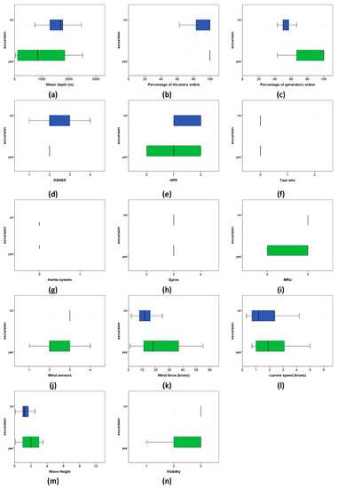
Figure 2.
Distribution of the potentially relevant variables stratified by whether excursion occurred: (a) Water depth, (b) Percentage of thrusters, (c) Percentage of generators, (d) GNSS, (e) HPR, (f) Taut wire, (g) Inertia system, (h) Gyros, (i) MRUs, (j) Wind sensors, (k) Wind force, (l) Current speed, (m) Wave height, and (n) Visibility.
Figure 3 shows the distribution of the causes of incidents stratified by whether they resulted in LoP. For loss-of-position incidents, the most common main cause category was environmental (7 cases, 53.8%), followed by human error (2 cases, 15.4%). For the incidents not resulting in a LoP, the most common main cause category was thruster faults (9 cases, 31.0%), followed by environmental conditions (6 cases, 20.7%), power faults (5 cases, 17.2%), and human error (4 cases, 13.8%).

Figure 3.
Distribution of incidents as a function of main (a) and secondary (b) cause stratified by whether excursion occurred.
In the case of the secondary causes, the cause category most often identified for loss-of-position incidents was reference system faults (2 incidents, 40% of all incidents with a secondary cause), while in the case of incidents not resulting in a LoP, the most common were human error or sensor faults (3 incidents each, 37.5% of all incidents with secondary cause).
Finally, the distribution of the incidents considering whether human error was considered to be a cause is represented in Figure 4. As described in Section 2.1, we classified the cause as “human” when either the main or the secondary causes were considered to be human operator error. Overall, in 33 cases (78.6%), no human error was identified, while in 9 cases (21.4%), human error was cited as a cause. For incidents resulting in an excursion, human error was not considered a cause in 10 cases (76.9%), but was identified in 3 cases (23.1%). Similarly, when there was no LoP, human error was considered to have been a cause of the incident in 23 cases (79.3%), while no human error was reported in 6 cases (20.7%).

Figure 4.
Distribution of incidents as a function of human error stratified by whether excursion occurred.
3.2. Binary Logistic Regression Model
First, the variables are entered into the model one by one, to check their significance in the model. The individual results are presented in Table 2.
Table 2.
Individual results for each independent variable when the binary regression model (method: Enter) is performed, with Excursion being the dependent variable.
At this stage, the variables that could be considered significant were: percentage of generators, wind force. At the same time, the size effect of variables like Water depth, Percentage of thrusters, and Wave height are also taken into account according to the observed CI.
The following variables are taken into account for creating the model: Water depth, Percentage of generators, Wind force, and Wave height, using the Enter mode.
The criteria followed for determining the variables that are significant for entering the model are to select those variables with a value different from 1 in the column OR. Values for OR above 1 indicate that when the predictive variable increases, there is a LoP; values below 1 show an excursion when the predictive variable decreases. When the CI comprises the value 1, it means that the variable predicts a LoP when increasing and decreasing at the same time, which makes it inadequate for the purpose of prediction.
For example, for Wind force, OR = 1.081 and for Current speed, OR = 1.176. However, the CI for Current speed does include the number 1, and thus is not considered to be explaining the model.
However, there are two cases in which the team considered the variables even though the above criteria were not met. For Water depth, taking into account that the CI limits were has not been very strict. For the variable Water depth, it was appreciated the CI did include 1 as the upper limit, and decided to select this variable. Wave height was also included as it is considered to be a weather variable, and the lower limit of the CI is relatively close to 1. Current speed, although it is also a weather variable, has the lower limit further from 1 and was not selected.
The statistics of the selected variables are presented in Table 3.
Table 3.
Variables in the equation in Step 2.
The following equation defines the model:
Z = −4.936 − 0.001∙Waterdepth + 0.058∙Percentage of generators − + 0.050 Wind force + 0.461 Wave Height.
The probability of excursion and the relative ratio are calculated according to Equations (2) and (6), taking into account that the relative ratio can also be expressed as follows,
P/Q = exp (4.936) ∙ exp (−0.001∙Waterdepth) ∙ exp(0.058∙Percentage of generators) + exp (0.050 Wind force) + exp (0.461 Wave Height).
Between 34% (Cox and Snell R square) and 48% (Nagelkerque R square) of the variance in the dependent variable is explained by this model. The goodness of fit was assessed by the −2LL statistic and the percentage of correctly classified cases. The −2LL was 34.355. Recalling that of the 42 valid cases, 29 incidents did not and 13 did result in an excursion, the model (based on the two variables selected) correctly classified 27 incidents as not involving excursion, meaning 93% of cases were correctly classified; while 8 cases were correctly classified as involving excursion, 62% of the total. Overall, 35 cases were correctly classified, representing 83% of the incidents studied. The Cohen’s kappa shows there is a moderate agreement between the P observed and P estimated values, κ = 0.584 (95% CI, 0.312 to 0.856).
Figure 5 shows graphically the model predictions for LoP for different values of water depth and percentage of generators.
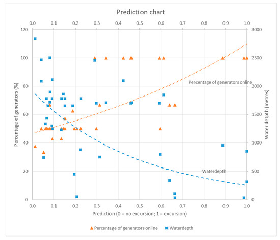
Figure 5.
Prediction chart showing the trends for water depth and percentage of generators according to the prediction model.
The relative ratio indicates the likelihood of LoP for each of the main causes, as shown in Figure 6. The dashed line makes it clear which causes have mean values above 1, those with a greater likelihood of being associated with a LoP. Overall, the main causes most likely to be related to an excursion are failures in environmental conditions, reference systems, human errors, and computer faults.

Figure 6.
Mean relative ratio for each main cause category.
4. Discussion
Selecting only the incidents with no missing information for any of the variables of interest, the database used for this study contained 42 cases. The descriptive analysis of the variables provides a comprehensive picture of the main configurations (percentage of thrusters, percentage of generators, DGNSS, etc.) used for DP drilling operations, including the typical meteorological conditions (wind force, current speed, wave height, and visibility) when an incident occurs.
Taking into account the nature of the accident, it is interesting to see that incidents attributable to poor environmental conditions have a clear tendency to result in LoP. In contrast, in incidents with causes related to thrusters/propulsion or power, control of positioning tends to be maintained. These results are consistent with the information regarding the most common causes of DP incidents provided by the IMCA in their station keeping reports [38,39,40,41,42].
The secondary causes are much less often identified, and the results involving them should be considered with caution. Nonetheless, our data seem to support the aforementioned conclusion that power-related incidents tend not to result in a LoP.
The distribution of incidents with human error as a cause is very similar; there are no significant differences for the incidents which do and do not result in LoP.
In the first stage, when the variables are individually entered into the regression model, the variables that might explain the probability of an excursion were found to be water depth, percentage of generators, wind force, and wave height; the first two related to the DP system configuration, and the second two to meteorological conditions. Percentage of generators and wind force are found to be clearly significant, while water depth and wind force are added to the model on the basis of their size effect. It should not be forgotten that the weather conditions, and especially the wind force (which creates waves with a height that is proportionally correlated to the force in knots), can also influence the probability of a unit having a LoP while performing DP drilling operations, as evidenced by the frequency of incidents attributable to environmental conditions.
The probability of an incident resulting in LoP increases the shallower the water depth, and the higher the percentage of generators, wind force and wave height. These results are very interesting from the operator’s point of view, as at shallow depths, DP has tended not to be considered necessary and other methods have been used to achieve position keeping. The resulting lack of experience in the use of DP under such conditions could partly explain problems occurring with DP station keeping when the drilling operations take place in shallow waters.
The percentage of generators online at the moment of an incident is also an indicator of a LoP when the percentage reaches high values. It is important to note that, according to the DP Operations Guidance [13], when the percentage of generators reaches a certain threshold, the procedures for a riser emergency disconnection should be started; this may explain the influence of this variable in the model.
Studying the mean relative ratios for each main cause category, it is interesting to note that the model can explain environmental-, reference-, human-, and computer-related incidents more accurately than those attributed to other causes. The high mean relative ratio for environmental-related LoP can be explained by the environmental independent variables included in the model. The reference faults present a high mean relative ratio as well. The correlation that exists between percentage of generators and wind sensors could be a hint for explaining this result. This influence is expected to be explained when performing the regression analysis using dummy variables for the different reference systems on board (gyros, MRUs, and wind sensors); future research in this area is therefore needed. In general, this model correctly classifies incidents as resulting or not resulting in excursion in 83% of cases, and therefore it is expected to perform well in predicting the outcome of this type of incident in real-world operations. However, the CI for Cohen’s kappa in this model shows that the predictive capability is not as high as the classification success indicates.
The correlation among variables shows that human error is not significantly connected with the variable excursion, but there is a high correlation with the variable percentage of thrusters. For this variable, it can be observed that the percentage is significantly smaller in cases with human error as a cause. This suggests that, had the output of the model been used for predicting whether the human error was involved in any incident, this would be one of the most influential variables in the model. Nonetheless, in this study, the results for percentage of thrusters cannot be considered to contribute significantly to explaining the LoP in any incident.
When the predictive variable is used for predicting excursions, the results obtained do not suggest that human errors are involved in LoP. This is also visible in the descriptive statistics, in Figure 4, as per the distribution of the variable stratified by excursion does not show any differences.
Limitations
This study is based upon a sample of 42 incidents taken from IMCA database. Due to the excellent safety measures in the drilling sector, the incidents involving DP are kept to a minimum. Such a great safety record, however, limits the data available and the sample for our study was composed of just 42 incidents which took place from 2011 to 2015, giving us a relatively small database. This is especially notable in the group of incidents with human error as a cause.
Following the work presented by Øvergård [51], the sample obtained is based on incidents, as non-incidents (i.e., events which worked as planned) are usually not worth recording. This selection bias can have an influence on the validity of the outcomes, as only a partial view of the operations is taken into account.
The method used offers some advantages over other methods described in the literature review, but at the same time there are some limitations that should be mentioned.
Regression models assume that the relationship between the predictor variables and the dependent variable is uniform, i.e., follows a particular direction—this may be positive or negative, linear or nonlinear but is constant over the entire range of values. In this context, the coefficients calculated in the model should be used with caution.
If the independent variables are highly correlated with one another (multicollinearity), then the effect of each becomes less precise. In our study, it was found that the observed data for expected correlated variables, such as Wind force and Wave height, were not highly correlated, although the correlation could be found for other pairs of variables without apparent relationship, such as Percentage of generators and Wind sensors. As these pairs of variables have not been considered at the same time in the model, it is expected that this effect has been minimized. The bigger impact of environmental conditions causing LoP cannot be denied, and the authors wanted to reflect this by including weather variables in all regression analysis, to have an overall view of the scores for each variable, even if they are not reaching the desired significance for entering the equation.
The predictive capability showed by the classification rates should be also considered with caution, as the Cohen’s kappa suggest there is a fair to moderate coincidence between the observed and the estimated classification, as the model is tested with the same database the analysis was performed on.
Some relationships between covariate and dependent variable can be disguised as non-significant due to low sample size rather than to statistical significance. In our case, with 42 cases, it is important to have an overall picture rather than to follow the cut-offs that the p-values offer. On this basis, variables like Wave height were selected to enter the model.
5. Conclusions
The main goal of this study was to determine a mathematical expression that explains the likelihood of a LoP during DP drilling operations.
Missing data could not be inferred because of the large number of variables and their complexity, none of them following a normal distribution. Nonetheless, the performance of the model in this sample (in terms of the percentage of correctly classified cases) increases our confidence in the prediction capability of the model. Taking into account the variables included in the database, we opted to use a binary logistic regression model, as in (8). With this model, it can be determined that the probability of LoP is associated with higher percentages of generators, wind force and wave heights, and shallower water depths.
Considering that a high percentage (83%) of cases is correctly classified by the model based on these variables, this model is expected to provide good results when predicting whether any incident will result in LoP. The incidents caused by environmental conditions, reference faults, human error, or computer faults are expected to be most successfully classified following the proposed model. This indicates that although the most common causes are environmental and thruster problems, the LoP occurs more often in environment-related incidents. This suggests that investigating which environmental conditions most influence LoP would be an interesting line of future research.
The last objective of this study was to explore whether or not human causes contribute to LoP. The results obtain suggest that there is not a clear connection among these variables; the human element causing an incident does not influence the prediction of LoP.
Author Contributions
Conceptualization, Z.S.-V., J.L.L.B., and M.A.G.-S.; Data curation, Z.S.-V.; Formal analysis, Z.S.-V. and D.B.-F.; Investigation, Z.S.-V. and D.B.-F.; Methodology, Z.S.-V. and D.B.-F.; Resources, Z.S.-V. and D.B.-F.; Software, Z.S.-V. and D.B.-F.; Supervision, J.L.L.B. and M.A.G.-S.; Visualization, Z.S.-V., D.B.-F., and J.L.L.B.; Writing—original draft, Z.S.-V., D.B.-F., and J.L.L.B.; Writing—review and editing, Z.S.-V., D.B.-F., J.L.L.B., and M.A.G.-S. All authors have read and agreed to the published version of the manuscript.
Funding
This research received no external funding.
Data Availability Statement
Restrictions apply to the availability of these data. Data was obtained from the International Maritime Contractors Association (IMCA) and are available at https://www.imca-int.com/store/digital-publications/.
Conflicts of Interest
The authors declare no conflict of interest.
Appendix A
Table A1.
Correlation coefficients (n = 42).
References
- Nie, Z.; Chang, Y.; Liu, X.; Chen, G. A DBN-GO approach for success probability prediction of drilling riser emergency disconnect in deepwater. Ocean. Eng. 2019, 180, 49–59. [Google Scholar] [CrossRef]
- United States Department of the Interior. Mineral Management Service. “Accident Investigation Report”. Available online: https://www.bsee.gov/sites/bsee.gov/files/incident-statisticssummaries-fatalities/inspection-and-enforcement/060320-pdf.pdf (accessed on 15 December 2020).
- Mac Sheoin, T.; Zavestoski, S. Chapter four: Corporate catastrophes from UC bhopal to BP deepwater horizon: Continuities in causation. corporate negligence. and crisis management. In Black Beaches and Bayous; Eargle, L.A., Esmail, A., Eds.; University Press of America: Lanham, MD, USA, 2012; pp. 53–94. [Google Scholar]
- Mauro, F.; Prpić-Oršić, J. Determination of a DP operability index for an offshore vessel in early design stage. Ocean. Eng. 2020, 195, 106764. [Google Scholar] [CrossRef]
- Chen, H.; Moan, T.; Verhoeven, H. Safety of dynamic positioning operations on mobile offshore drilling units. Reliab. Eng. Syst. Saf. 2008, 93, 1072–1090. [Google Scholar] [CrossRef]
- Verhoeven, H.; Chen, H.; Moan, T. Safety of dynamic positioning operation on mobile offshore drilling units. In Proceedings of the MTS Dynamic Positioning Conference, Houston, TX, USA, 17–18 October 2006. [Google Scholar]
- Chae, C. A Study on Human Error of DP Vessels LOP Incidents. J. Korean Soc. Mar. Environ. 2015, 21, 515–523. [Google Scholar] [CrossRef]
- Chae, C. A Study on FSA Application for Human Errors of Dynamic Positioning Vessels Incidents. J. Navig. Port. Res. 2017, 41, 259–268. [Google Scholar] [CrossRef]
- Dong, Y.; Vinnem, J.E.; Utne, I.B. Improving safety of DP operations: Learning from accidents and incidents during offshore loading operations. Eur. J. Decis. Process. 2017, 5, 5–40. [Google Scholar] [CrossRef]
- Øvergård, K.I.; Sorensen, L.J.; Nazir, S.; Martinsen, T.J. Critical incidents during dynamic positioning: Operators’ situation awareness and decision-making in maritime operations. Theor. Issues Ergon. Sci. 2015, 16, 366–387. [Google Scholar] [CrossRef]
- Mao, L.; Zeng, S.; Liu, Q. Dynamic mechanical behavior analysis of deep water drilling riser under hard hang-off evacuation conditions. Ocean Eng. 2019, 183, 318–331. [Google Scholar] [CrossRef]
- Bray, D. DP Operations. Part 2—What is DP used for? Seaways 2018, 9, 13–16. [Google Scholar]
- Marine Technology Society. DP Operations Guidance—Part 2—Appendix 1–MODUs; Marine Tecnology Society: Washington, DC, USA, 2012. [Google Scholar]
- Bray, D. DP Operations. Part 1—Basic Principles and Systems. Seaways 2018, 8, 22–25. [Google Scholar]
- Weingarth, L. Refining the DP watch circle. In Proceedings of the MTS Dynamic Positioning Conference, Houston, TX, USA, 17–18 October 2006. [Google Scholar]
- Bhalla, K.; Cao, Y. Watch circle assessment of drilling risers during a drift-off and drive-off event of a dynamically positioned vessel. In Proceedings of the MTS Dynamic Positioning Conference, Houston, TX, USA, 15–16 November 2005. [Google Scholar]
- Quigley, C.; Williams, D. A Revised Methodology for the Calculation of Modu Watch Circles. In Proceedings of the ASME 2015 34th International Conference on Ocean Offshore and Arctic Engineering, St. John’s, NL, Canada, 31 May–5 June 2015; The American Society of Mechanical Engineers, 2015; p. V05AT04A008. [Google Scholar] [CrossRef]
- Adamson, A.; Abrahamsen, B. WSOG—History and future. A summary of the development & worldwide use of well-specific operating guidelines. In Proceedings of the MTS Dynamic Positioning Conference, Houston, TX, USA, 17–18 October 2006. [Google Scholar]
- Teixeira, F.J.R.; Oshiro, A.T.; Tannuri, E.A. Drifting Time of a Standard Drillship. In Proceedings of the ASME 2014 33rd International Conference on Ocean Offshore and Arctic Engineering, San Francisco, CA, USA, 8–13 June 2014; The American Society of Mechanical Engineers, 2014. Volume 1B: Offshore Technology. p. V01BT01A029. [Google Scholar] [CrossRef]
- Kristiansen, S. Part III. Risk Analysis. In Maritime Transportation; Safety Management and Risk Analysis; Elsevier Butterworth-Heinemann: Oxford, UK, 2005. [Google Scholar]
- Khan, F.I.; Abbasi, S.A. Techniques and methodologies for risk analysis in chemical process industries. J. Loss Prev. Process Ind. 1998, 11, 261–277. [Google Scholar] [CrossRef]
- Ancione, G.; Bragatto, P.; Milazzo, M.F. A Bayesian network-based approach for the assessment and management of ageing in major hazard establishments. J. Loss Prev. Process Ind. 2020, 64, 104080. [Google Scholar] [CrossRef]
- Mkrtchyan, L.; Podofillini, L.; Dang, V.N. Bayesian belief networks for human reliability analysis: A review of applications and gaps. Reliab. Eng. Syst. Saf. 2015, 139, 1–16. [Google Scholar] [CrossRef]
- Bier, V.M.; Mosleh, A. The analysis of accident precursors and near misses: Implications for risk assessment and risk management. Reliab. Eng. Syst. Saf. 1990, 27, 91–101. [Google Scholar] [CrossRef]
- Bier, V.M.; Yi, V.M. The performance of precursor-based estimators for rare event frequencies. Reliab. Eng. Syst. Saf. 1995, 50, 241–251. [Google Scholar] [CrossRef]
- Khakzad, N.; Khakzad, S.; Khan, F. Probabilistic risk assessment of major accidents: Application to offshore blowouts in the Gulf of Mexico. Nat. Hazards 2014, 74, 1759–1771. [Google Scholar] [CrossRef]
- Yang, M.; Khan, F.; Lye, L.; Amyotte, P. Risk assessment of rare events. Process Saf. Environ. Prot. 2015, 98, 102–108. [Google Scholar] [CrossRef]
- Arnaldo Valdés, R.M.; Liang Cheng, S.Z.Y.; Gómez Comendador, V.F.; Sáez Nieto, F.J. Application of Bayesian Networks and Information Theory to Estimate the Occurrence of Mid-Air Collisions Based on Accident Precursors. Entropy 2018, 20, 969. [Google Scholar] [CrossRef]
- Rebello, S.; Yu, H.; Ma, L. An integrated approach for real-time hazard mitigation in complex industrial processes. Reliab. Eng. Syst. Saf. 2019, 188, 297–309. [Google Scholar] [CrossRef]
- Shengli, L.; Yongtu, L. Exploring the temporal structure of time series data for hazardous liquid pipeline incidents based on complex network theory. Int. J. Crit. Infrastruct. Prot. 2019, 26, 100308. [Google Scholar] [CrossRef]
- Agarwal, S.; Kachroo, P.; Regentova, E. A hybrid model using logistic regression and wavelet transformation to detect traffic incidents. IATSS Res. 2016, 40, 56–63. [Google Scholar] [CrossRef]
- Li, R.; Pereira, F.C.; Ben-Akiva, M.E. Competing risks mixture model for traffic incident duration prediction. Accid. Anal. Prev. 2015, 75, 192–201. [Google Scholar] [CrossRef]
- McFadden, K.L. Predicting pilot-error incidents of US airline pilots using logistic regression. Appl. Ergon. 1997, 28, 209–212. [Google Scholar] [CrossRef]
- Erjavac, A.J.; Iammartino, R.; Fossaceca, J.M. Evaluation of preconditions affecting symptomatic human error in general aviation and air carrier aviation accidents. Reliab. Eng. Syst. Saf. 2018, 178, 156–163. [Google Scholar] [CrossRef]
- Hogenboom, S.; Rokseth, B.; Vinnem, J.E.; Utne, I.B. Human reliability and the impact of control function allocation in the design of dynamic positioning systems. Reliab. Eng. Syst. Saf. 2020, 194, 106340. [Google Scholar] [CrossRef]
- Weng, J.; Yang, D.; Chai, T.; Fu, S. Investigation of occurrence likelihood of human errors in shipping operations. Ocean Eng. 2019, 182, 28–37. [Google Scholar] [CrossRef]
- Boullosa-Falces, D.; Larrabe-Barrena, J.L.; Lopez-Arraiza, A.; Menendez, J.; Gomez-Solaetxe, M.A. Monitoring of fuel oil process of marine diesel engine. Appl. Therm. Eng. 2017, 127, 517–526. [Google Scholar] [CrossRef]
- International Marine Contractors Association (IMCA). Dynamic Positioning Station Keeping Incidents—Incidents Reported for 2011; IMCA: London, UK, 2015; Available online: https://www.imca-int.com/store/digital-publications/marine/ (accessed on 27 June 2017).
- International Marine Contractors Association (IMCA). Dynamic Positioning Station Keeping Incidents—Incidents Reported for 2012; IMCA: London, UK, 2015. [Google Scholar]
- International Marine Contractors Association (IMCA). Dynamic Positioning Station Keeping Incidents—Incidents Reported for 2013; IMCA: London, UK, 2015. [Google Scholar]
- International Marine Contractors Association (IMCA). Dynamic Positioning Station Keeping Incidents—Incidents Reported for 2014; IMCA: London, UK, 2016. [Google Scholar]
- International Marine Contractors Association (IMCA). Dynamic Positioning Station Keeping Review—Incidents and Events Reported for 2015; IMCA: London, UK, 2016. [Google Scholar]
- International Marine Contractors Association (IMCA). Dynamic Positioning Station Keeping Review—Incidents and Events Reported for 2016; IMCA: London, UK, 2017. [Google Scholar]
- Marine Forecasts Glossary. Available online: https://www.metoffice.gov.uk/weather/guides/coast-and-sea/glossary (accessed on 10 December 2020).
- Menard, S. Applied Logistic Regression Analysis, 2nd ed.; Sage Publications Inc.: Thousand Oaks, CA, USA, 2002. [Google Scholar]
- Martín-Martín, Q.; Cabero-Morán, M.T.; de Paz-Santana, Y.R. Capítulo 9. Regresión Logística. In Tratamiento Estadístico de Datos Con SPSS; Ediciones Paraninfo: Madrid, Spain, 2008; pp. 259–292. [Google Scholar]
- Halsey, L.G. The reign of the p-value is over: What alternative analyses could we employ to fill the power vacuum? Biol. Lett. 2019, 15, 20190174. [Google Scholar] [CrossRef]
- Kmetz, J.L. Correcting Corrupt Research: Recommendations for the Profession to Stop Misuse of p-Values. Am. Stat. 2019, 73, 36–45. [Google Scholar] [CrossRef]
- Lewis, N.D.C. Operational Risk with Excel and VBA: Applied Statistical Methods for Risk Management; John Wiley & Sons: Hoboken, NJ, USA, 2004. [Google Scholar]
- Steyerberg, E.W.; Vickers, A.J.; Cook, N.R.; Gerds, T.; Gonen, M.; Obuchowski, N.; Pencina, M.J.; Kattan, M.W. Assessing the Performance of Prediction Models: A Framework for Traditional and Novel Measures. Epidemiology 2010, 21, 128–138. [Google Scholar] [CrossRef]
- Øvergård, K.I. Human Error: Causality and the Confusion of Normative and Descriptive Accounts of Human Performance. In Creating Sustainable Work Environments; Fostervold, K.I., Johnsen, S.Å.K., Rydstedt, L., Watten, R.G., Eds.; Norwegian Society for Ergonomics and Human Factors: Lillehammer, Norway, 2015; pp. C5-6–C5-10. [Google Scholar]


Publisher’s Note: MDPI stays neutral with regard to jurisdictional claims in published maps and institutional affiliations. |
© 2021 by the authors. Licensee MDPI, Basel, Switzerland. This article is an open access article distributed under the terms and conditions of the Creative Commons Attribution (CC BY) license (http://creativecommons.org/licenses/by/4.0/).