Abstract
In this work, the hydrodynamic performance of a novel wave energy converter (WEC) configuration which combines a moonpool platform and a javelin floating buoy, called the moonpool–javelin wave energy converter (MJWEC), was studied by semianalytical, computational fluid dynamics (CFD), and experimental methods. The viscous term is added to the potential flow solver to obtain the hydrodynamic coefficients. The wave force, the added mass, the radiation damping, the wave capture, and the energy efficiency of the configuration were assessed, in the frequency and time domains, by a semianalytical method. The CFD method results and the semianalytical results were compared for the time domain by introducing nonlinear power take-off (PTO) damping; additionally, the viscous dissipation coefficients under potential flow could be confirmed. Finally, a 1:10 scale model was physically tested to validate the numerical model and further prove the feasibility of the proposed system.
1. Introduction
The increasing need to replace traditional fossil fuels with clean energy (including wind, tidal, and wave energy) for power generation has been highlighted in the last ten years. Among the different kinds of marine energies, wave energy has become one of the most promising options that can be regarded as a resource component. Wave energy converters (WECs) can be used to extract wave energy through the periodic resonance caused by slow periodic waves. The wave energy is utilized via WECs, which can convert wave energy in sea water into electrical energy. As energy conversion devices, they can adapt to the wave conditions of the selected sea area, absorb wave energy stably and reliably, and realize the energy conversion to the maximum extent. Several classic devices based upon the theory of wave conversion are the Archimedes Wave Swing [1], CETO [2], the IPS Buoy [3], and the Wavebob [4].
The problem of hydrodynamic interaction between waves and cylindrical structures has been the subject of academic research because of its wide and important applications in various engineering projects. Several conceptual studies have been carried out to improve its efficiency. Ramadan et al. [5] designed a new float which consists of two parts, a hollow cylinder and an inverted cup attached to its bottom. Mavrakos and Katsaounis [6] investigated the different effects of floaters’ geometries by analyzing the performance of tight-moored vertical axisymmetric WECs. The results showed the effect of the different hydrodynamic characteristics of each specific float geometry on the studied hydroelectric performance characteristics. Zang and Zhang [7] studied the power performance of a heaving-buoy WEC with power take-off (PTO) damping under regular and irregular waves.
To consider viscous effects, potential-flow theory can be introduced as a dissipative term in the boundary conditions, where the dissipative term acts as a fictitious dissipative force to suppress the kinetic energy associated with wave uplift. When the resonance occurs in a confined region, the amplitude of the fluid motion is reduced. Duan et al. [8] improved the method and calculate the wave loads associated with the wave elevation by introducing uncertainties to the free surface conditions in the case of a set of cylinders. Chen et al. [9] applied a semianalytical method based on eigenfunction matching to study the wave diffraction of cylindrical structures with a moonpool by introducing dissipation to the free-surface conditions. Liu et al. [10] introduced a nonlinear viscous dissipation term in the modeling of the free surface inside the lunar pool structure and derived the relationship between the nonlinear dissipation coefficient and the resonant frequency of the lunar pool. The CFD method is, however, more accurate compared with the above method; Lo et al. [11] used a CFD approach to analyze the performance of an air-blower wave power generation device, and to calculate the power output of two buoys. Jin et al. [12] took the nonlinear viscosity into account to model the WEC hydrodynamics’ near-resonance conditions.
The experimental approach is a useful method for conducting feasibility studies on newly developed WECs. Ren et al. [13] analyzed the combination of a monopile wind turbine and a swing-type WEC and derived the optimal tuning of the PTO damping by using a coordinated numerical and experimental analysis. Gao et al. [14] studied three floating wind–wave hybrid concepts, comparing their energy efficiency and economic feasibility. Wan et al. [15,16,17] studied the green water phenomena of STC, and a model test was used to simulate these nonlinear phenomena as well as the survivability of the device in extreme sea conditions.
It is difficult to use conventional methods to explore two floating coupling resonances from a mechanism and optimize the PTO damping to improve the power. Few studies have taken into account the viscous effects of the potential-flow approach applied to the fundamental physics of the coupling resonance between two objects. In this paper, a semianalytical method introducing viscous dissipation to obtain a more accurate and efficient calculation method was used. Applying the Impulse Response Function (IRF) method, the motion responses of a moonpool–javelin wave energy converter (MJWEC) were determined by employing time–history analysis. Theoretical analysis, numerical calculation, and model testing were combined and compared, highlighting the underpinning physics of the coupling resonance between the two bodies.
2. Mathematical and Numerical Model
This paper is focused on the MJWEC, as seen in Figure 1—the moonpool platform and a javelin floating buoy on the water surface, connected by the PTO system. The motion responses of the moonpool and the javelin float to waves were of multiple degrees of freedom (DOFs). In this paper, only the heaving DOF was considered, which was the most important parameter related to the power take-off of the device.

Figure 1.
MJWEC and its basin division.
A sketch of the structure layout for the WEC is shown in Figure 1. It was a javelin float model, having a vertical axisymmetric floating body containing a cylinder and a “Berkeley Wedge” bottom. The surfaces could be obtained by creating a shape function; the fourth-order polynomial is as follows:
According to Madhi et al. [18], we chose the appropriate buoyancy and sharpness to make , , and . The radius and draught of the javelin float are and . The external structure in Figure 1 is a moonpool platform, which is a hollow cylinder coaxially placed on the periphery of the javelin float. The inner and outer radii are and the draught is . The water depth is . The origin o is defined as the intersection between the central axis of the floating body and the hydrostatic surface, and a Cartesian coordinate system and a cylindrical coordinate system were established, respectively. The oz axes of the two floats were vertically aligned with the central axis. The Cartesian coordinate system plane and cylindrical coordinate system plane coincided with the hydrostatic surface by the and conversion relationship.
2.1. Semianalytical Solution in Frequency Domain
2.1.1. Diffraction Problems
As shown in Figure 1, we divided the flow field around the javelin float into four parts , , , and . Within the four parts, we divided the subdomain P into N parts. The diffraction wave velocity potential could be written as:
By substituting the boundary conditions, we could obtain the series expression of the diffraction velocity potential of E and M:
where , is the first type of Bessel function, and is the second type of Bessel function. We used the following equation to solve and :
in which,
By substituting the boundary conditions, we could obtain the series expression of the diffraction velocity potential of B:
where,
When we solved the diffraction velocity potential of P, the diffraction velocity potential of and had different boundary conditions, so we discuss their diffraction velocity potential separately. Using boundary conditions, we could obtain:
From the above formula, where , we could obtain:
Within these formulae, we still had Fourier series , , , and to solve. They were solved by the continuity conditions of the adjacent subdomain velocity potential and their derivative, and the lateral surface conditions. The continuity conditions between the adjacent subarea interface were:
The impenetrable conditions on the side surface of the object were:
The velocity potential and the partial derivative continuity condition at the coupling interface of the javelin float bottom domain could be written as:
The number of velocity potentials at the coupling interface should satisfy the continuity condition and the condition of the float surface. Using Green’s function, the orthogonality of the velocity potential function was applied to obtain the analytical expression of the diffraction velocity potential. The wave force received by the moonpool platform and the javelin float in the waves was obtained by the Bernoulli equation:
2.1.2. Radiation Problems
Similarly to the diffraction problem, based on the uniform propagation of energy around the wave motion, the radiation velocity potential in the wave state could be expressed as:
Substituting the boundary conditions, we could obtain:
where , , , , and refer to the diffraction problem. Meanwhile, the special solution for each radiation velocity potential was:
In the coupling plane of each subdomain, the boundary conditions and diffraction problems were consistent. At the same time, they also met the impervious conditions:
due to the continuity of the velocity potential derivative at the coupling interface. Using the Green’s function method and the orthogonality of the function, we obtained the unknown Fourier coefficients for the radiation velocity potential. Then, we could obtain the series expressions of the radiation velocity potential:
where and represent additional mass and radiation damping. The subscript stands for the moonpool platform radiation acting on the javelin float. The rest of the subscripts signify the same thing as . The potential-flow theory does not take into account viscosity and energy dissipation. The value of the hydrodynamic calculation of the floating body under the ideal fluid conditions would be relatively large, and there would be significant distortion for the motion under resonance. In order to improve the accuracy of the potential-flow calculation results, a damped-cover method based on the pseudo-ideal fluid assumption was used to achieve a viscous correction effect by adding damping between the moonpool platform and the javelin float.
2.1.3. Motion Equation and Capture Width Ratio
As shown in Figure 2, the MJWEC in this paper was connected by a PTO damping system to form a Double-degree-of-freedom damped vibration system.
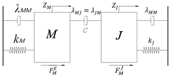
Figure 2.
Double-degree-of-freedom vibration system.
The MJWEC mets the equilibrium state in still water. When it was subjected to waves, it made a heave motion. The displacement caused by the heave motion was the distance between the instantaneous position of the float and the equilibrium position. On this basis, the microwave was satisfied. According to Newton’s second law, the motion equation in the frequency domain could be expressed as:
where and represent the quality of the MJWEC, respectively; and represent the displacement of the moonpool platform and the javelin float relative to their hydrostatic equilibrium state; and represent the wave excitation force of the moonpool platform and the javelin float; , and represent the radiation force of the moonpool platform on itself, the radiation force of the moonpool platform on the javelin float, the radiation force of the javelin float on the moonpool platform, and the radiation force of the javelin float on itself. They could be written as:
where and represent the hydrostatic stiffness of the lunar platform and the javelin float. When the water line area of the float was constant, they could be expressed as ρ and g, representing the representative seawater density and gravitational acceleration, respectively. could be expressed as the speed-dependent damping force. Assuming that the PTO damping coefficient c was linear, substituting the Formulas (40)–(42) for Formula (39), we could obtain:
After separating the time variable, the MJWEC equation of motion could be expressed as:
The MJWEC was connected by the PTO system. Under the action of waves, the relative motion of the two floats used the displacement difference between the two to drive the damper in the PTO system to generate electricity. The power could be expressed as:
where is the incident wave frequency, and are the magnitude of the motion response of the moonpool platform and the javelin float, and c is the PTO damping coefficient.
When studying the influence of the size of the moonpool platform on the conversion efficiency of the wave energy device, only the influence of the output power could not be measured. Therefore, the concept of the capture width ratio could be introduced to better determine the wave energy conversion of the device. The ratio of the capture width represents the ratio of the average output power of the float to the power of the wave input within the corresponding float width. In Cartesian coordinates, the waveform of the incident wave with amplitude , frequency w, and phase angle δ was as follows:
Then, the energy input in the unit period and the float width was derived from the following equation:
The capture width ratio of the wave frequency w was:
2.2. Time-Domain Solutions
Based on the device sketch in Figure 1, the frequency-domain motion equations were established. The rotation axis o was taken as the reference point. For the wave energy device studied in this article, we established the time-domain motion equation as follows:
where and represent the quality of the moonpool platform and the javelin float, respectively; , and indicate the time domain added mass; represents the delay function; and the subscript indicates the radiation effect of the front object on the back object. The signs , and represent the displacement, velocity, and acceleration, respectively. The signs , , and represent the hydrostatic force coefficient of the lunar platform and the javelin float. and represent the wave forces acting on the moonpool platform and the javelin float. indicates the linear instantaneous PTO damping force acting on the moonpool platform–javelin float device, and denotes in the linear condition. However, the actual situation of the PTO system involved a quadratic damping force and an even more complicated variation law. To more realistically simulate the mechanical motion of the whole system, the nonlinear PTO was decomposed into a secondary damping force:
Then, the equation could be transformed into:
The equation could be solved using the fourth order Runge–Kutta method.
2.3. Introduce Dissipation in Potential Flow
To eliminate the sharp resonance and to measure the viscous effect of the moonpool–javelin wave energy converter (MJWEC), dissipation was introduced into the potential flow by assuming an additional term in the boundary condition at the free surface of the moonpool. According to Chen and Dias [19], the boundary condition on the mean free surface for the potential is modified velocity potential after adding the viscous solveras summarized in the introduction, by introducing a dissipative term:
where the symbol is the dissipation coefficient and . When the sharp resonance phenomenon appears, introducing a dissipative term reduces the motion of the fluid in a narrow space. The dispersion equation associated with the new free-surface boundary condition (53) became:
where the symbols and are the wavenumbers, and this dispersion Equation (54) became a complex relation. The attenuation factor that affected the imaginary part of the wavenumber appeared:
in which the real part of the wavenumbers and satisfied the usual dispersion equation,
The imaginary part was given by:
It is important to note that, in the semianalytical solution for wavenumbers and , all the Bessel functions mentioned became the complex variable Bessel function. Additionally, if the dissipation coefficient μ = 0, the imaginary parts of the wavenumbers and were zero and the semianalytical solution for introducing dissipation into the potential flow was equal to the semianalytical solution under potential flow.
2.4. Computational Fluid Dynamics (CFD) Method
2.4.1. Reynolds Averaged Navier–Stokes (RANS) Equations
Based on Figure 1, the frequency-domain motion equations were established. The rotation axis o was taken as the reference point. The unsteady incompressible flow field was described by the continuity equation and the Navier–Stokes equations,
where is the water density, is the flow velocity vector, is the body force vector, and is the stress tensor. Starting from Navier–Stokes equations, and imposing the continuity equation, the Cauchy momentum equation could be derived. Then, assuming that the water density was constant in space (incompressible) and in time, the expression (58) was obtained.
An unsteady RANS-based CFD model (Star-CCM+) was used to model fluid flow, where the governing equations were discretized over a computational mesh using a finite-volume method. The results were found to be in good agreement with the available experimental results in the literature. A volume of fluid (VOF) method was applied to calculate the free surface, and a mesh-morphing model was adopted to represent the moving boundary between the liquid and the central cylindrical buoy, which was moving. A Lagrangian–Eulerian method was implemented to handle the cell movement. A SIMPLE-type algorithm was applied to solve the system of equations, where the dynamic response of the floating body was calculated by integrating (over time) the acceleration obtained from the equation of motion solution, using an implicit algorithm.
2.4.2. Computational Domain and Boundary Conditions
Figure 3 shows the computational domain and domain boundaries of the numerical wave tank used in the RANS simulations. To reduce the computational cost and exploit the problem symmetry, only half of the domain was modeled. The computational domain was 108 m long, 7 m wide, and 1.5 m high. As regards the boundary conditions (Figure 3), the seabed was 1.5 m below the mean water surface, nonpenetration and a no-slip condition boundary condition was imposed, and a 5th order Stokes wave velocity profile was specified at the inflow. The pressure outlet was implemented at the outflow boundary.

Figure 3.
Computational domain and domain boundaries.
2.4.3. Mesh Generation
The mesh generation was performed using the automated mesh facility in Star-CCM+, resulting in a computational mesh with a total of about 14 million cells. A trimmed cell grid was used to generate a high-quality grid for complex grid generation problems. The ensuing mesh was formed primarily of unstructured hexahedral cells with trimmed cells adjacent to the surface. Figure 4 shows the grid resolution around the MJWEC model. The grid resolution was finer near the free surface and around the model, to capture both the wave dynamics and the details of the flow around the WEC. In addition, prism-layer cells were placed along the WEC surface, and the height of the first layer was set so that the value of y + (30~100) satisfied the turbulence model requirement.
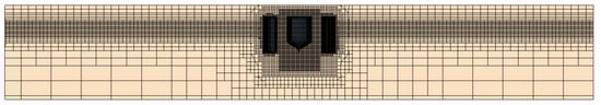
Figure 4.
Grid around the MJWEC mode.
3. Numerical Results and Discussion
3.1. Dynamic Characteristic Analyses in the Frequency Domain
3.1.1. The Hydrodynamic Characteristic
In this section, we only study the relative motion between the moonpool platform and the javelin float. We set the water depth at and the seawater density at ; the waves were linear microwaves, their frequency was , and the wave height was . During the research, we kept the moonpool platform horizontal thickness at . When the wave energy device draught remained, , the inner diameter , and the PTO damping coefficient remained at . When the inner diameter of the wave energy device was maintained at , the draught of the device was and the PTO damping coefficient remained at . When the moonpool size remained fixed at , we changed the PTO damping coefficient to . The calculation results are dimensionlessly expressed as and .
The Influence of ’s Change on the Force of the Devices
In Figure 5, (a) stands for the wave force on the moonpool and (b) for the wave force on the sea javelin.
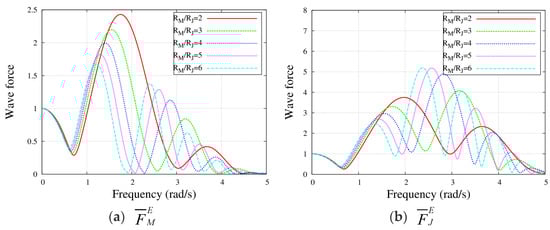
Figure 5.
Variation of wave force with frequency on the moon pool platform and sea javelin for different radius ratios.
The wave forces on the moonpool platform all varied from 1. Three peaks appeared as the frequency increased, and the size of each peak decreased as the frequency increased. For the first peak, the size of the peak decreased with the increasing frequency as the radius increased, and the frequency corresponding to the peak also decreased with the increasing frequency. The peak corresponded to a range of frequencies. For the wave force received by the javelin float, there were also two to three peaks, but the value of the second peak was significantly larger than that of the other peaks. When the radius increased, the value of the peak increased gradually, and the frequency corresponding to the peak also increased gradually. It can be seen that the wave force variation pattern was the same for the moonpool platform and the javelin float, and the variation pattern was opposite at different wave peaks. In the low frequency state, the moonpool platform and the javelin float had the same frequency, corresponding to a very small value for the wave force. Furthermore, the wave force on the moonpool platform was larger than that on the javelin float at the same frequency.
The Influence of ’s Change on the Force of the Devices
In Figure 6, (a) stands for the wave force on the moonpool and (b) for the wave force on the sea javelin.

Figure 6.
Variation of wave force with frequency on moon pool platform and sea javelin for different draft ratios.
From Figure 6a, we can see that for the wave force received by the moonpool platform, the peak values of the first and second peak points decreased with the increase in the draught, but the frequency corresponding to the peak point changed only slightly, and the frequency of the first peak point was around . The second peak-point frequency was around . From Figure 6b, the value of the wave force received by the javelin float decreased with the increase in the draught at the first peak point, but the value of the second peak point hardly changed with the draught.
The Influence of ’s Change on Hydrodynamic Coefficients of the Devices
Figure 7a,b represent the added mass and radiation damping of the moonpool, (c) and (d) the added mass and radiation damping between the moonpool and the sea javelin, and (e) and (f) the added mass and radiation damping of the sea javelin.
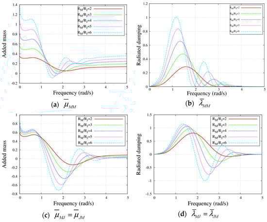

Figure 7.
The hydrodynamic coefficients of the moonpool platform and the sea javelin.
As shown in Figure 7, the increased mass first decreased, then increased with the frequency, and finally stabilized. Moreover, the frequency range is , the size of the added mass changes very little, and increases with the increase of the radius. When the frequency range was , the additional mass first decreased and then increased, and the peak value decreased with the increase in the radius. When the frequency range was , the additional mass tended to be stable and changed very little with the increase in the radius. The radiation damping first increased and then decreased with the increase in the frequency, and there were two peaks of magnitude. The magnitude of the peak increased with the increase in the radius, while the frequency of the peak point decreased. It is worth noting that the additional mass and the radiation-damping radius of the javelin float were the same when the radiation effect of the javelin float was on itself.
The Influence of ’s Change on Hydrodynamic Coefficients of the Devices
Figure 8a,b represent the added mass and radiation damping of the moonpool, (c) and (d) the added mass and radiation damping between the moonpool and the sea javelin, and (e) and (f) the added mass and radiation damping of the sea javelin.

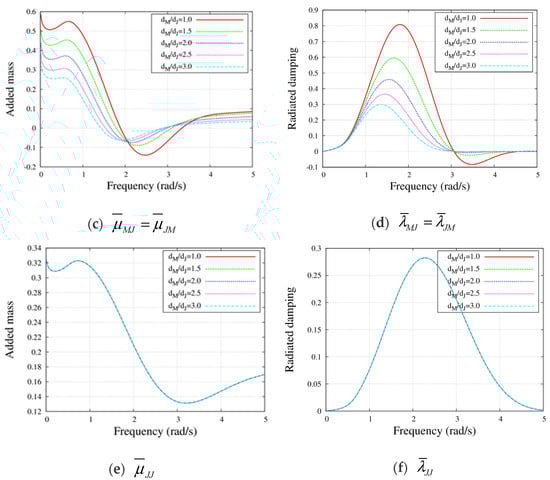
Figure 8.
The hydrodynamic coefficients of the moonpool platform and the float.
As shown in Figure 8, the increased mass first decreased, then increased with the frequency, and finally stabilized. Furthermore, the frequency range was —the size of the added mass changed very little and decreased with the increase in the draught. When the frequency range was , the additional mass first decreased and then increased, and the peak value increased with the increase in the radius. When the frequency range is the additional mass tended to be stable and changed very little with the increase in the radius. The radiation damping first increased and then decreased with the increase in the frequency, and there were two peaks of magnitude. The peak value decreased with the increase in the radius, while the frequency of the peak point also showed a decreasing trend. In conclusion, a comparison between Figure 7 and Figure 8e,f shows that the size of the moonpool had no effect on the additional mass and radiation damping when the radiation generated by the javelin float was applied to the moonpool itself, and the short, thick moonpool platform had a large radiation damping force.
3.1.2. The Motion Response
The results of the response amplitude operator were given by Equation (44), which could be used to verify the influence of the geometrical parameter of the moonpool and javelin damping coefficients on the wave energy buoy motion.
As can be seen from Figure 9, the overall trend is the same regardless of whether the radius of the moon pool platform or the draft changes, and there are one or two peaks. When a given moonpool platform drew water, as the radius increased, the value of the first peak point increased, while the frequency corresponding to the peak point decreased. The change law of the second peak point was the same. When the radius of a given lunar pool platform was calculated, the value of the first peak point increased with the increase in the draught and the frequency corresponding to the peak point decreased with the increase in the draught, while the second peak point did not change with it. The motion response rate of the moonpool platform was greater than that of a single javelin float in the range of frequency , so the moonpool platform could improve the dynamic characteristics of the device within a certain range of wave frequency.
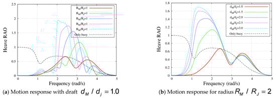
Figure 9.
The motion response of the MJWEC for different radius ratios and draft ratios.
Based upon the previous calculation, the optimum MP dimension could be obtained, so the measure of the MP was the radius and the draught , and the measure of the WEB and wave condition remained unchanged. Figure 10 shows the motion response for the MP and the WEB with various PTO damping coefficients (c = 20, 40, 60, 80, and 100()) and various frequencies (), respectively.
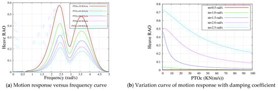
Figure 10.
Effect of damping and frequency on motion response of the MJWEC.
It can be seen from the figure on the left that, under different PTO damping coefficients, when the wave frequency occurred , the relative motion amplitude of the moonpool float tended to be 0 m. When the wave frequency was zero, the curve kept rising and reached the first peak point when the wave frequency was zero. The peak value decreased with the increase in the PTO damping coefficient. When the frequency was , the second peak point was reached, which was lower than the first peak and decreased with the increase in the PTO damping coefficient. As can be seen from the figure on the right, the trend of the motion response is the same for different frequencies depending on the PTO damping factor. When the frequency was constant , the amplitude of the motion response decreased with the increase in the PTO damping coefficient and kept decreasing until it approached 0. When the wave frequency was , the motion response was much larger than the motion response at other frequencies. At this wave frequency, the PTO damping coefficient of 100 reduced the motion response by 0.51 m.
3.1.3. The Capture Width Ratio
The results of the capture width ratio were given by Equation (49), which could be used to verify the influence of the geometrical parameter of the MP and SJ damping coefficient.
As can be seen from the Figure 11a, when the moonpool’s draught was constant, the peak value of the first peak point initially increased and then decreased with the increase in the radius. This was because when the radius increased, the input power of the incident wave also increased, but the frequency corresponding to the peak point decreased with the increase in the radius. When the wave frequency range was , the wave energy efficiency captured by the moonpool platform device was better than that of a single javelin float. It can be seen from the figure on the right that there were two obvious peaks in the capture width ratio of the floating device of the moonpool, which were caused by the resonance between the platform of the moonpool and the javelin float, and the frequency of the resonance point was not consistent. When the radius is fixed, as the month draft increases, the first peak value increases, but the second peak value reduces, rate of change is relatively small, peaks corresponding to the frequency of the peak in the first place have changed, but the peak in the second place, there is no change that the first peak point related to the moonpool platform resonance, the second peak point related to the javelin floating buoy resonance.
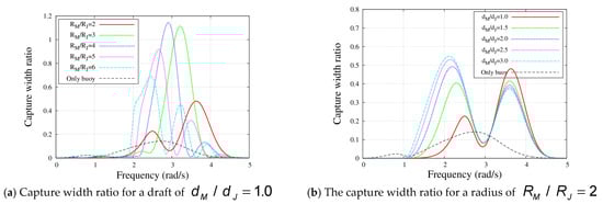
Figure 11.
The capture width ratio of the MJWEC for different radius ratios and draft ratios.
As can be seen from the Figure 12 on the left, under the conditions of different PTO damping coefficients, when the wave frequency was , the first peak appeared in the capture width ratio of the moonpool float. With the increase in the PTO damping coefficient, the peak gradually decreased. When the wave frequency of occurred, the second peak value appeared on the capture width ratio curve. The effect of the PTO damping coefficient on the peak value was smaller than that on the first peak value. The third peak was the same as the second peak. As can be seen from the Figure 12 on the right, when the wave frequency was , the motion response of the device was significantly higher than that of the other wave frequencies with the change of the PTO damping coefficient, and when the damping coefficient was , the motion response rapidly increased and then slowly decreased. When the wave frequencies were and , the motion response of the device increased with the increase in the PTO damping coefficient, but the increase rate was small. When the wave frequencies were and , the motion response of the device increased with the increase in the PTO damping coefficient, but the increase rate was small.
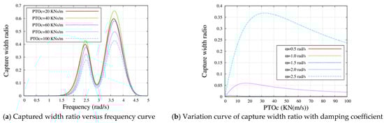
Figure 12.
Effect of damping and frequency on the capture width ratio of the MJWEC.
3.2. Dynamic Characteristic Analyses in the Time Domain
3.2.1. The Motion Response
In this section, the MP-WEB is introduced and equation (50) is solved.. The dissipation coefficients were and .
As can be seen from Figure 13, the four graphs (a)–(d) showed roughly the same change trends, but the changes under forced motion were still different, due to the effect of adding viscous damping. After stabilization, it can be seen from the comparison of Figure 13a,b that the damping coefficient played an inhibitory role in the amplitude of the instantaneous motion response, and the larger the value of , the stronger the effect of amplitude reduction. In order to find a more suitable dissipation coefficient, experiments should be carried out to discover the optimal value. For the later time-domain calculation, the viscous dissipation coefficient was selected as the fixed value for the subsequent calculation.

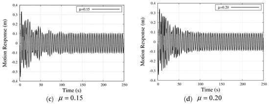
Figure 13.
The motion response of the MJWEC with different dissipation coefficients.
The numerical results were derived using Star-CCM+ software for comparison with the time-domain results achieved via the Potential-Flow Viscous Dissipation (PFVD) method.
As shown in Figure 14, it can be seen from the CFD calculation results that the instantaneous motion response of the moonpool float showed irregular changes at the beginning but gradually became stable over time, and the curve change period after stabilization decreased with the increase in the frequency. When the frequency was low, the peak of the curve deviated and the two peaks were different. When the frequency was high, the curve showed a periodic reciprocating motion, and the phase difference was the same. A comparison between the CFD calculation method and the method based on potential-flow theory for the introduction of viscous dissipation showed that the amplitudes of the two methods were very close. Comparatively speaking, the CFD calculation result was larger than that of the potential-flow analysis algorithm for viscous dissipation. At the same time, there was a phase difference between the curves of the two methods, which was caused by the wave phase during the calculation. Compared with the CFD method, the convergence time is shorter.

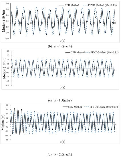
Figure 14.
The motion response with different frequencies.
3.2.2. The Capture Width Ratio
According to Equation (49), the different dissipation coefficients could be applied to obtain the capture width ratio over time. In addition, the equipment parameters were the same as above.
It can be seen from Figure 15 that the four pictures (a)–(d) show roughly the same change trends, but the changes were still different under forced motion, due to the effect of adding viscous damping. After stabilization, it can be seen from the comparison of Figure 15a,b that the damping coefficient played an inhibitory role in the amplitude of the capture width ratio, and the higher the value, the stronger the effect of amplitude reduction. To find a more suitable dissipation coefficient, experiments should be carried out to discover the optimal value. For the later time-domain calculation, the viscous dissipation coefficient was selected as the fixed value for the subsequent calculation.

Figure 15.
The capture width ratio of the MJWEC with different dissipation coefficients.
The numerical results were derived using Star-CCM+ software for comparison with the time-domain results achieved via the PFVD method.
In Figure 16, the calculation results of the dissipated potential-flow method and the CFD method are compared. Since the potential-flow method had a long stable-convergence time, the capture width ratio in the selected time period was . As can be seen from the figure, the capture width ratio of the moonpool float showed irregular changes at the beginning but gradually became stable over time, and the change period of the curve after stabilization decreased with the increase in the frequency. A comparison of the curves obtained by the two methods showed that the period after stabilization was the same, but the amplitudes were different. The capture width ratio obtained by the CFD method was smaller than that obtained by the method of introducing dissipative potential flow. The potential-flow method for introducing viscous dissipation did not take into account the energy dissipation caused by the viscous effect at the bottom of the moonpool platform device.
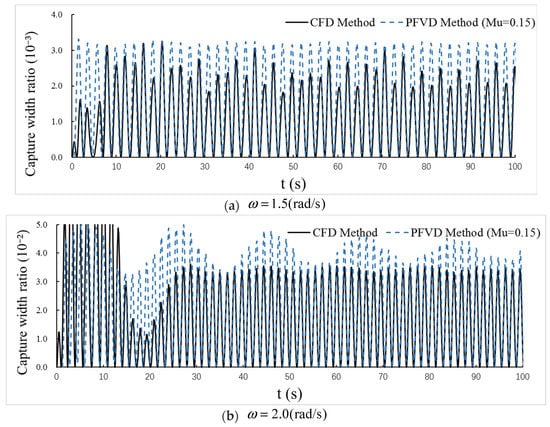
Figure 16.
The capture width ratio of the MJWEC with different frequencies.
4. Experimental Process and Results
4.1. Experimental Facility
The experiments considered here were carried out in the wave tank at Harbin Engineering University, which has a length and width of 108 m and 7 m, respectively. The depth of the test section was 1.5 m as shown in Figure 17. The push-type wave maker could generate waves with a height of up to 0.4 m and period between 0.4 and 4.0 s. The irregular waves that could be generated could model ITTC, JONSWAP, and P–M wave spectra with a wave height between 0 and 0.32 m.
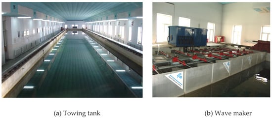
Figure 17.
Experimental facilities.
4.2. Wave Parameter
At the first approximation, and under the conditions tested, it could be assumed that a linear relationship existed between the wave amplitude and the motion response of the tested device, and therefore, the motion response amplitude operators (RAOs) could be defined. The wave height was 0.12 m and the wave periods ranged from 1.2 s to 3.0 s, as shown in Table 1. A total number of 14 working conditions were considered in the model test.

Table 1.
The working conditions.
4.3. Experimental Results
The influence of the wave period on the motion displacement and output power of the moonpool float was studied. Figure 18 shows the displacement curve and the power curve of the moonpool float device.

Figure 18.
The motion response and capture width ratio with different wave periods.
As can be seen from Figure 18, when the period of the high-frequency part was 1.2 s–1.9 s, the period had a great influence on the displacement and power of the javelin float, and the greater the period, the greater the displacement and power of the moonpool float. When the period of the low-frequency part was 2.2 s–3.0 s, the larger the period was, the smaller the displacement and output power of the moonpool float. When the period of the low-frequency part is 2.2 s–3.0 s, the larger the period is, the smaller the displacement and output power of the moonpool floater will be. When the cycle is 1.9 (s) and 2.4 (s), the motion and power appeared two peaks, the device has the highest energy conversion efficiency, the period of actual waters 5.985 and 7.56 (s) accordingly, higher the wave height is, higher the output power of the moonpool floater, which is of great significance for the follow-up study of similar devices. A comparison between the displacement and output power of the wave energy device of the moonpool float and the javelin float showed that when the period was 1.8 s–2.4 s, the displacement and power of the moonpool float were significantly higher than those of the javelin float, even reaching about two times higher at the peak. Therefore, the application of the moonpool platform in actual wave energy devices in engineering could effectively improve their energy conversion efficiency.
As can be seen from Figure 19, the amplitude of the temporal instantaneous motion response calculated by the viscous modified potential-flow method was very close to the value obtained by the model test, but the amplitude of the oscillation obtained by the theoretical calculation was larger than that obtained by the model test. Because the phase of the wave was different, there was a phase difference between the two curves. By comparing the time-domain relative displacements for different viscous dissipation coefficients with the results of the model test method, the appropriate viscous dissipation correction coefficients were selected as .

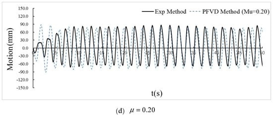
Figure 19.
Motion response of MJWEC with different dissipation correction factors over time.
5. Conclusions
In this paper, to improve the efficiency of converting energy from ocean waves, a new moonpool was adopted in the MJWEC. The diffraction and radiation of the linear wave caused by the MJWEC in water were examined in accordance with a semianalytical method. Case studies with different geometry parameters of the moonpool paddocks were verified. Mechanistic research was obtained for the PTO system regarding its energy conversion characteristics. Furthermore, CFD and experimental methods could be adopted to verify the accuracy of the PFVD method.
The results indicate:
- (1)
- A comparison of axisymmetric buoys with and without a moonpool platform showed that the moonpool had an effect on the hydrodynamic coefficient of the central buoy. For the frequency-domain dynamic characteristics of the MJWEC under potential flow, when the wave frequency was , the motion and capture width ratio of the wave energy device with the moonpool platform were significantly better than those of the single javelin float.
- (2)
- For CFD analysis, the platform device of the moonpool did not change the wave period inside the platform of the moonpool, but it did change the wave height inside the platform, improving the motion amplitude of the float. Therefore, the platform device of the moonpool significantly improved the energy conversion quality of the whole wave energy device. The CFD calculation method and viscous dissipation method based on potential-flow theory were very close to each other in terms of the amplitude of the motion response. Comparatively speaking, the CFD calculation result was higher than the potential-flow analysis algorithm for viscous dissipation.
- (3)
- According to the analysis of the test results of the model test, according to the linear wave theory, the influence of the wave height on the motion response and power of the MJWEC was positively linear. The wave period’s effects on different devices were not the same; a single javelin float peaked at 1.6 s, while the MJWEC had two peaks at 2.0 s and 2.4 s. Contrastingly, two experiments found that for certain wave periods from 1.8 s to 2.4 s, the javelin float performed better than the MJWEC in terms of displacement and power. Considering the peak values in particular, which were two times higher for the moonpool, the moonpool platform, when applied to the engineering practice of wave energy devices, could effectively improve the efficiency of their energy conversion. By comparing the results of the viscous dissipation and the pool test, the optimal viscous dissipation coefficient was found to be suitable.
Author Contributions
Conceptualization, D.Y. and K.W.; methodology, F.K.; software, Y.J.; validation, H.C., C.Y. and K.W.; formal analysis, K.W.; investigation, C.Y.; resources, Y.J.; data curation, H.C.; writing—original draft preparation, K.W.; writing—review and editing, F.K.; visualization, K.W.; supervision, F.K.; project administration, C.Y.; funding acquisition, Y.J. All authors have read and agreed to the published version of the manuscript.
Funding
This research received no external funding.
Institutional Review Board Statement
Not applicable.
Informed Consent Statement
Not applicable.
Data Availability Statement
Not applicable.
Acknowledgments
This paper was financially supported by the National Natural Science Foundation (grant No.52101306, No.52071095, and No. 51979063), the basic research and cutting-edge technology projects of the State Administration of Science (grant No.JCKY2019604C003), and the funds of the National Key Laboratory on Ship Vibration and Noise, China (6142204190207).
Conflicts of Interest
The authors declare no conflict of interest.
References
- Rademakers, L.W.; Van Schie, R.G.; Schuitema, R.; Vriesema, B.; Gardner, F. Physical Model Testing for Characterising the AWS; Netherlands Energy Research Foundation ECN: Petten, The Netherlands, 1998. [Google Scholar]
- Penesis, I.; Manasseh, R.; Nader, J.R.; de Chowdhury, S.; Fleming, A.; Macfarlane, G.; Hasan, M.K. Performance of ocean wave-energy arrays in Australia. In Proceedings of the 3rd AsianWave and Tidal Energy Conference (AWTEC 2016), Singapore, 24–28 October 2016; Volume 1, pp. 246–253. [Google Scholar]
- Cleason, L.; Forsberg, J.; Rylander, A. Contribution to the theory and experience of energy production and transmission from the buoy-concept. In Proceedings of the 2nd International Symposium on Wave Energy Utilization, Trondheim, Norway, 22–24 June 1982; pp. 345–370. [Google Scholar]
- Muliawan, M.J.; Gao, Z.; Moan, T. Analysis of a two-body floating wave energy converter with particular focus on the effects of power take-off and mooring systems on energy capture. J. Offshore Mech. Arct. Eng. 2013, 135, 317–328. [Google Scholar] [CrossRef]
- Ramadan, A.; Mohamed, M.H.; Abdien, S.M.; Marzouk, S.Y.; El Feky, A.; El Baz, A.R. Analytical investigation and experimental validation of an inverted cup float used for wave energy conversion. Energy 2014, 70, 539–546. [Google Scholar] [CrossRef]
- Mavrakos, S.A.; Katsaounis, G.M. Effects of floaters’ hydrodynamics on the performance of tightly moored wave energy converters. IET Renew. Power Gener. 2009, 4, 531–544. [Google Scholar] [CrossRef]
- Zang, Z.; Zhang, Q.; Qi, Y.; Fu, X. Hydrodynamic responses and efficiency analyses of a heaving-buoy wave energy converter with PTO damping in regular and irregular waves. Renew. Energy 2018, 116, 527–542. [Google Scholar] [CrossRef]
- Duan, W.Y.; Liu, H.X.; Li, R.P.; Chen, X.B. Wave loading on a group of cylinders in fairly perfect fluid[C] 10th International Conference on Hydrodynamics. Petersburg 2012, 10, 178–183. [Google Scholar]
- Chen, X.B.; Liu, H.X.; Duan, W.Y. Semi-analytical solutions to wave diffraction of cylindrical structures with a moonpool with a restricted entrance. J. Eng. Math. 2015, 90, 51–66. [Google Scholar] [CrossRef]
- Liu, H.X.; Chen, H.L.; Zhang, L.; Zhang, W.C.; Liu, M. Quadratic Dissipation Effect on the Moonpool Resonance. China Ocean Eng. 2017, 31, 665–673. [Google Scholar] [CrossRef]
- Lo, D.C.; Hsu, T.; Yang, C. Hydrodynamic Performances of Wave Pass Two Buoys-Type Wave Energy Converter. In Proceedings of the 27th International Ocean and Polar Engineering Conference, San Francisco, CA, USA, 25–30 June 2016; pp. 25–30. [Google Scholar]
- Jin, S.; Patton, R.J.; Guo, B. Viscosity effect on a point absorber wave energy converter hydrodynamics validated by simulation and experiment. Renew. Energy 2018, 129, 500–512. [Google Scholar] [CrossRef]
- Ren, N.; Ma, Z.; Fan, T.; Zhai, G.; Ou, J. Experimental and numerical study of hydrodynamic responses of a new combined monopile wind turbine and a heave-type wave energy converter under typical operational conditions. Ocean Eng. 2018, 159, 1–8. [Google Scholar] [CrossRef]
- Gao, Z.; Moan, T.; Wan, L.; Michailides, C. Comparative numerical and experimental study of two combined wind and wave energy concepts. J. Ocean Eng. Sci. 2015, 1, 36–51. [Google Scholar] [CrossRef] [Green Version]
- Wan, L.; Greco, M.; Lugni, C.; Gao, Z.; Moan, T. A combined wind and wave energy-converter concept in survival mode: Numerical and experimental study in regular waves with a focus on water entry and exit. Appl. Ocean Res. 2017, 63, 200–216. [Google Scholar] [CrossRef]
- Wan, L.; Gao, Z.; Moan, T. Experimental and numerical study of hydrodynamic responses of a combined wind and wave energy converter concept in survival modes. Coast. Eng. 2015, 104, 151–169. [Google Scholar] [CrossRef] [Green Version]
- Wan, L.; Gao, Z.; Moan, T.; Lugni, C. Experimental and numerical comparisons of hydrodynamic responses for a combined wind and wave energy converter concept under operational conditions. Renew Energy 2016, 93, 87–100. [Google Scholar] [CrossRef]
- Madhi, F.; Sinclair, M.E.; Yeung, R.W. The “Berkeley Wedge”: An asymmetrical energy-capturing floating breakwater of high performance. Mar. Syst. Ocean Technol. 2014, 9, 5–16. [Google Scholar] [CrossRef]
- Chen, X.B.; Dias, F. Visco-potential flow and time-harmonic ship waves. In Proceedings of the 25th International Workshop on Water Waves and Floating Bodies, Harbin, China, 9–12 May 2020. CNKI:SUN:HEBD.0.2010-01-011. [Google Scholar]
Publisher’s Note: MDPI stays neutral with regard to jurisdictional claims in published maps and institutional affiliations. |
© 2021 by the authors. Licensee MDPI, Basel, Switzerland. This article is an open access article distributed under the terms and conditions of the Creative Commons Attribution (CC BY) license (https://creativecommons.org/licenses/by/4.0/).