Numerical Investigation of Internal Solitary Wave Forces on Submarines in Continuously Stratified Fluids


Abstract
:1. Introduction
2. Numerical Model of an ISW in Continuously Stratified Fluid
2.1. Governing Equations
2.2. Numerical Methods
2.3. Initialised Field of ISW Generation
3. Model Verification
3.1. Computational Settings for SUBOFF Simulation
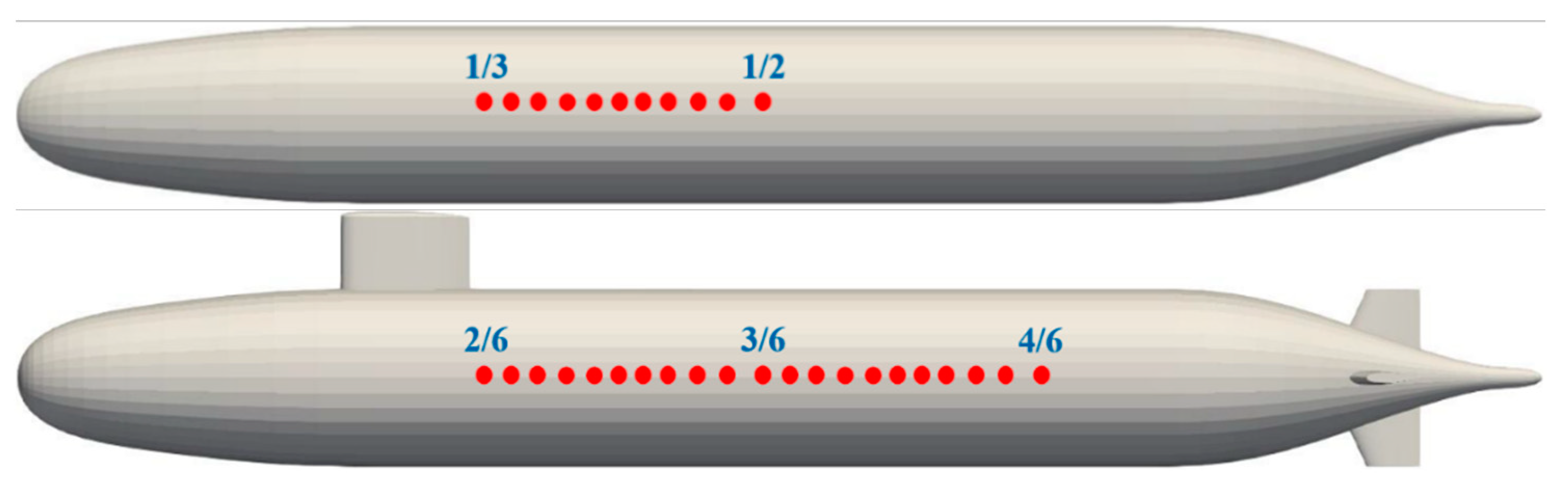
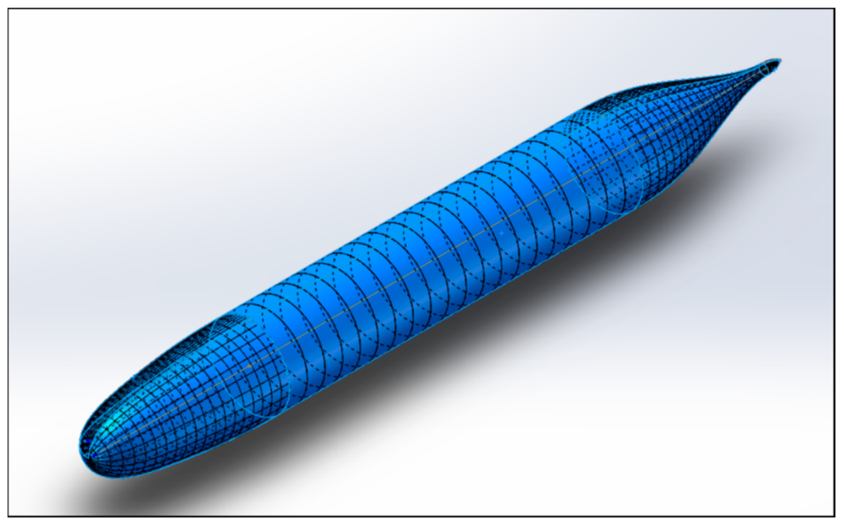
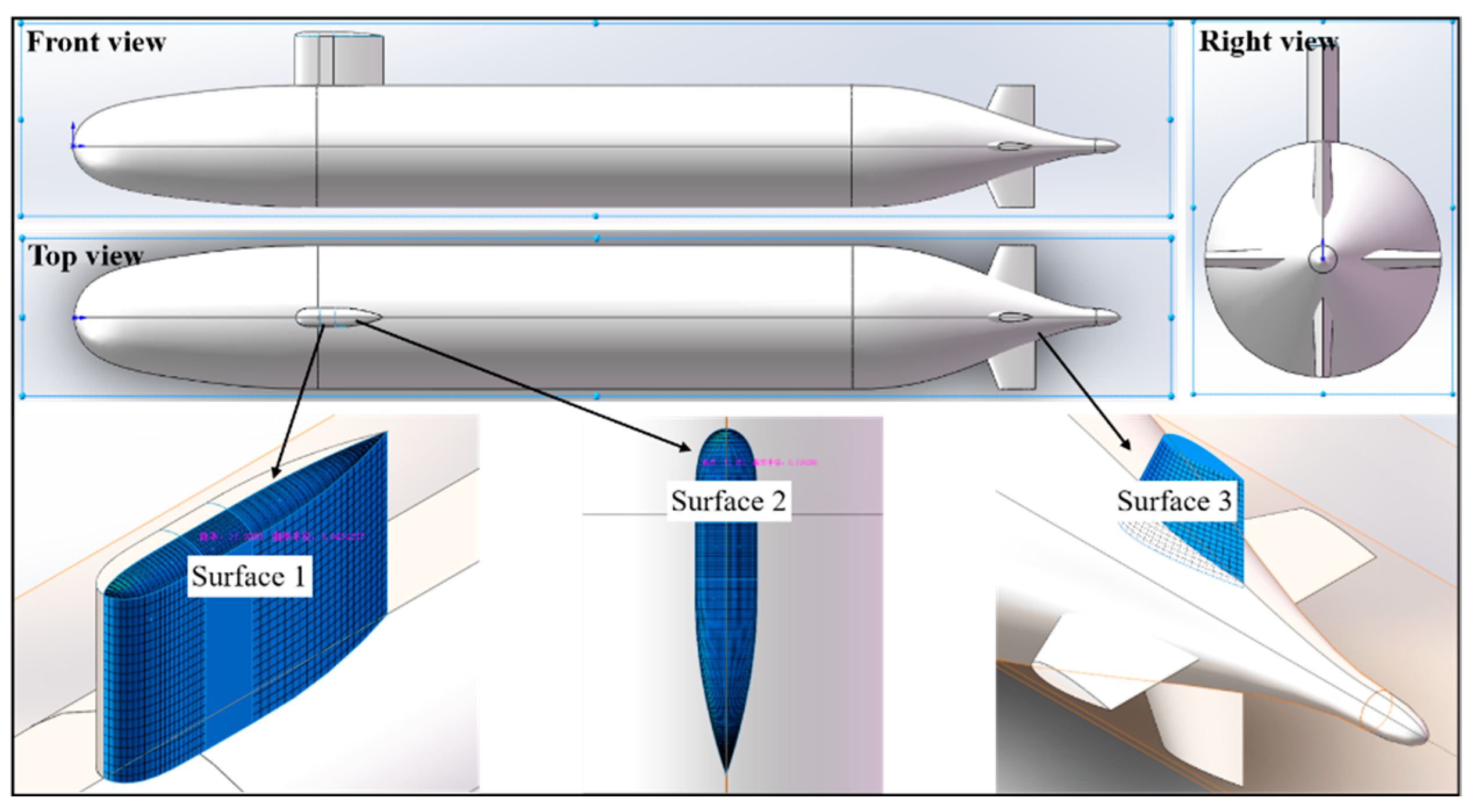
3.1.1. About the SUBOFF Model
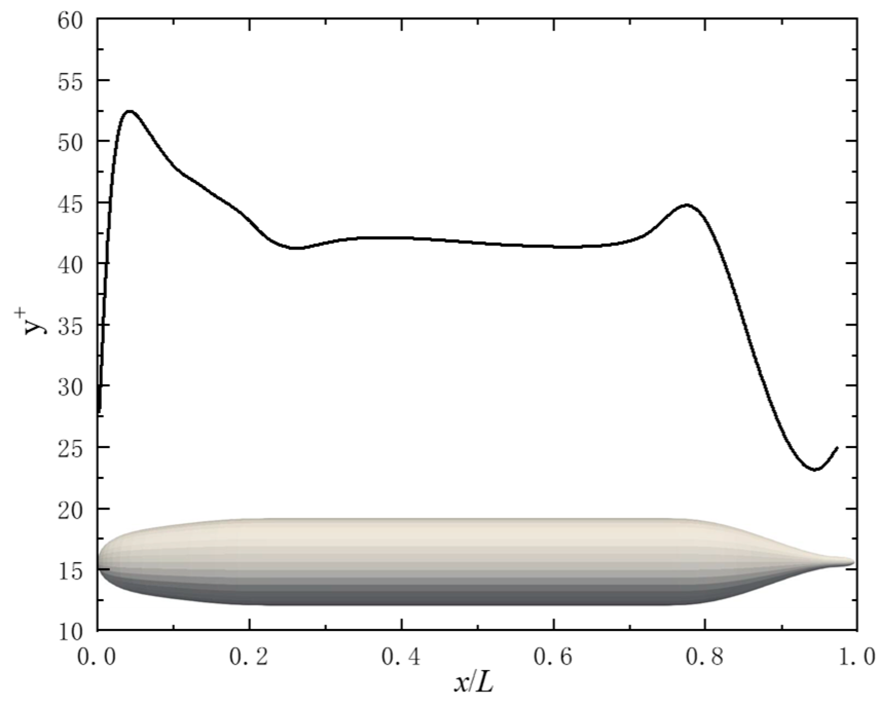
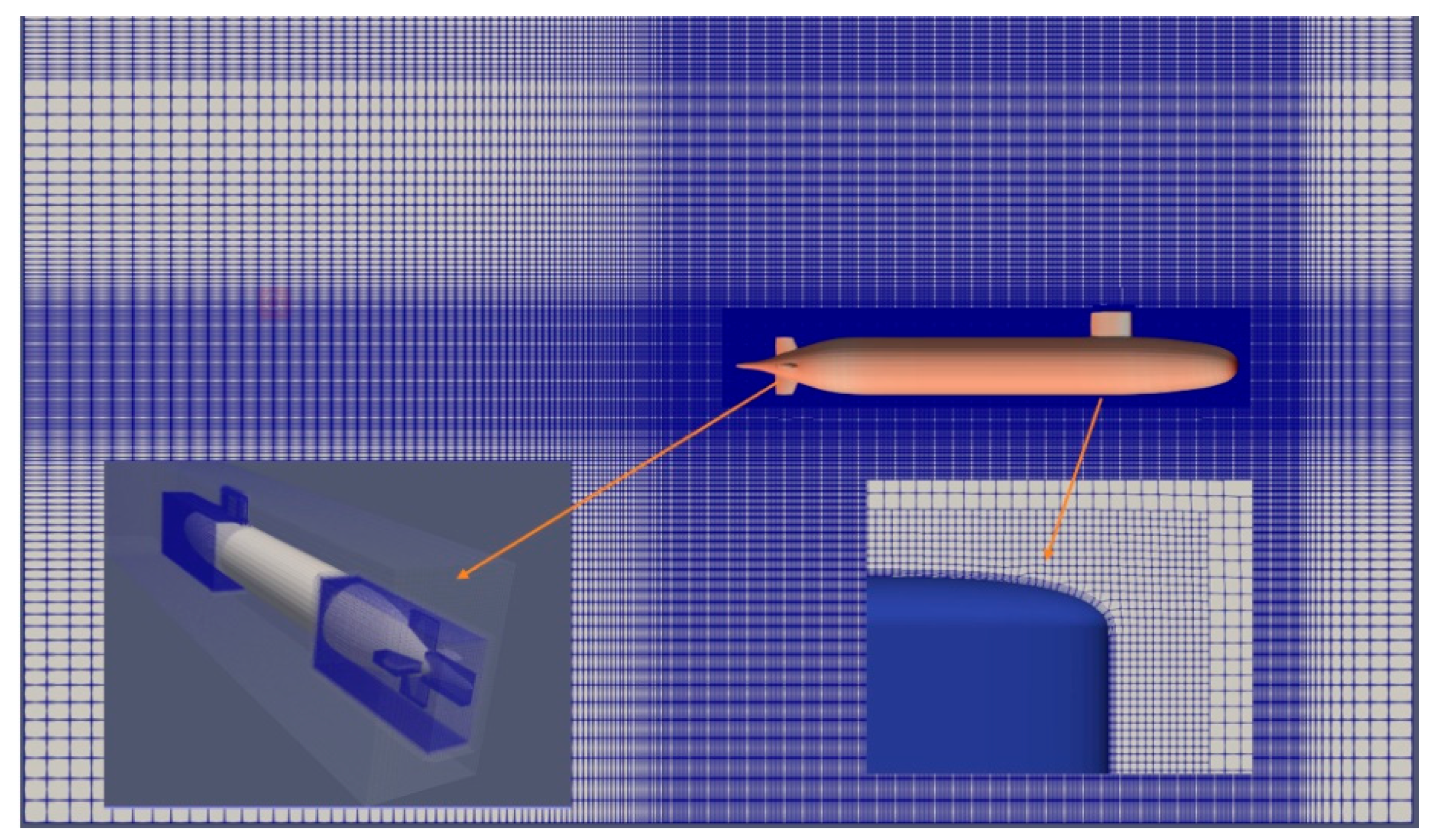
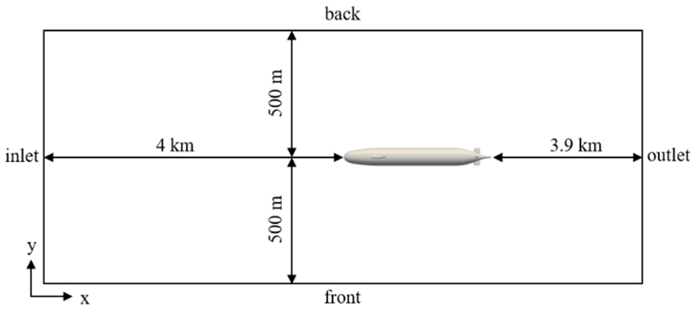
3.1.2. Computational Domain and Grids
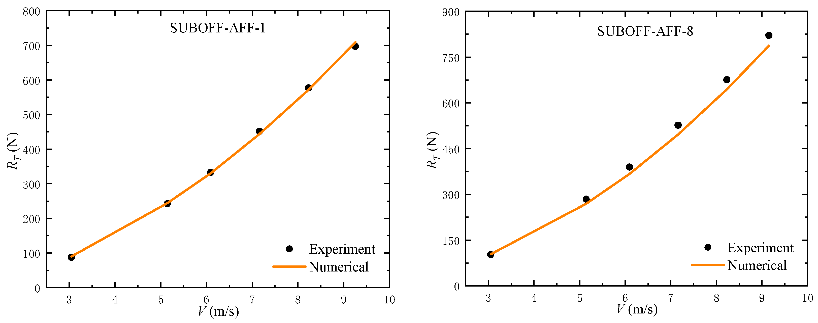
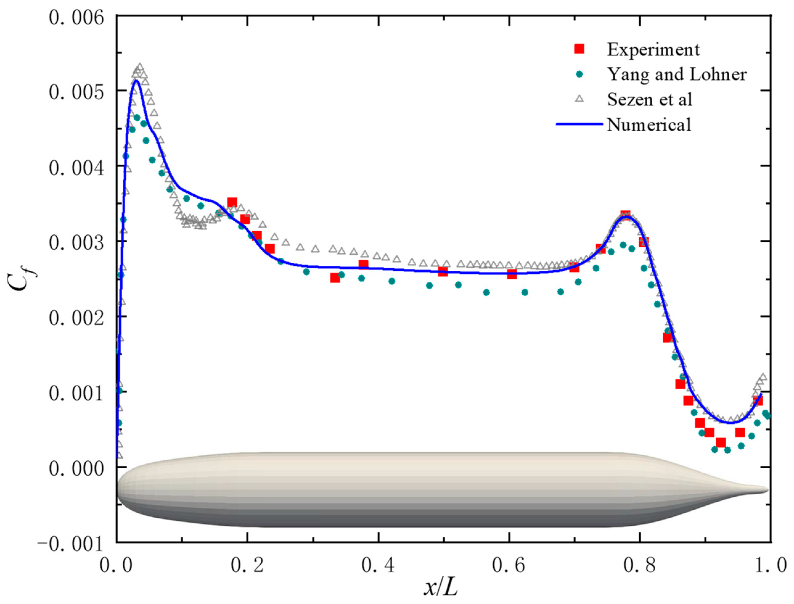
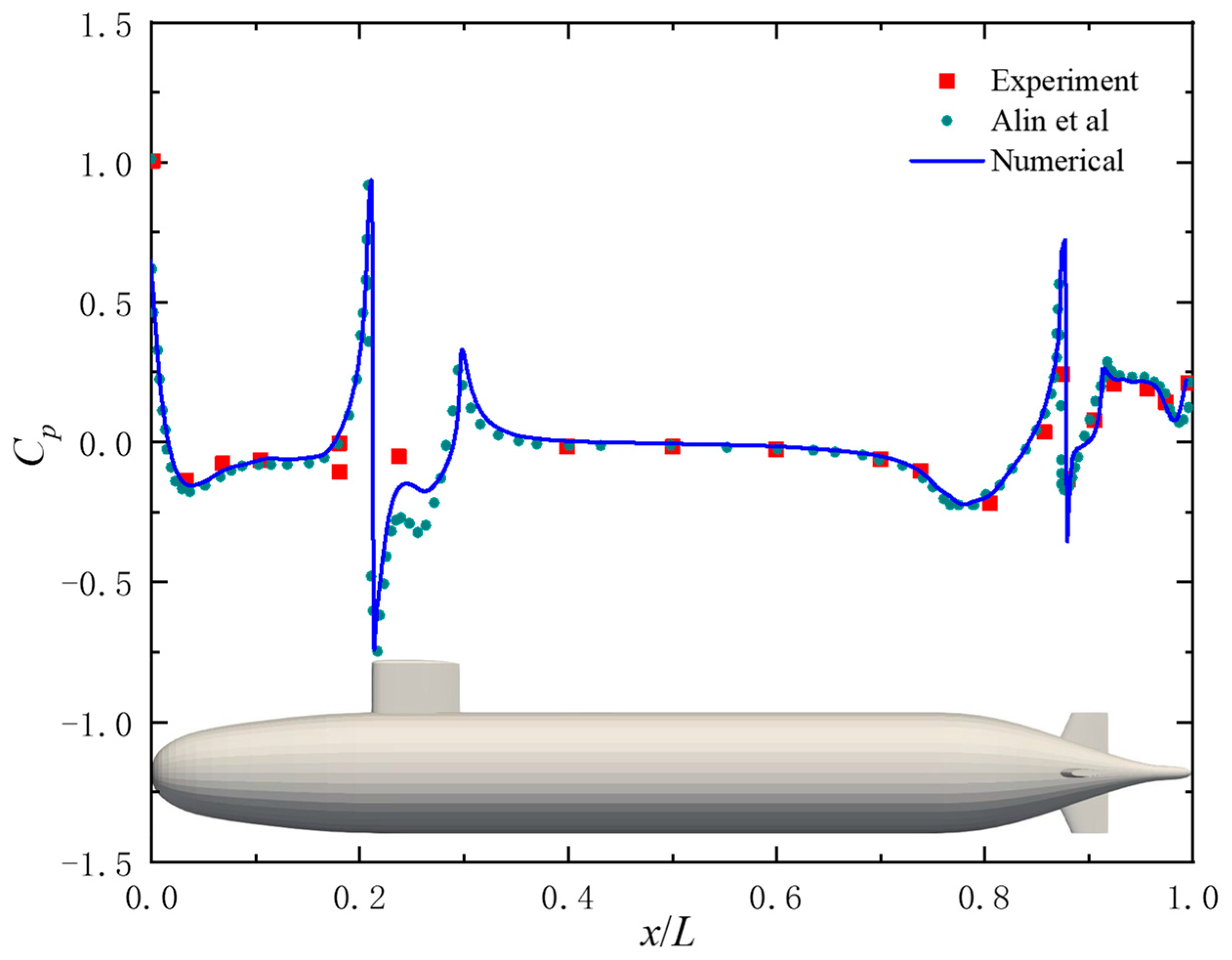
3.2. Comparisons between Simulated and Measured Results
4. Numerical Analysis of ISW Forces on SUBOFF
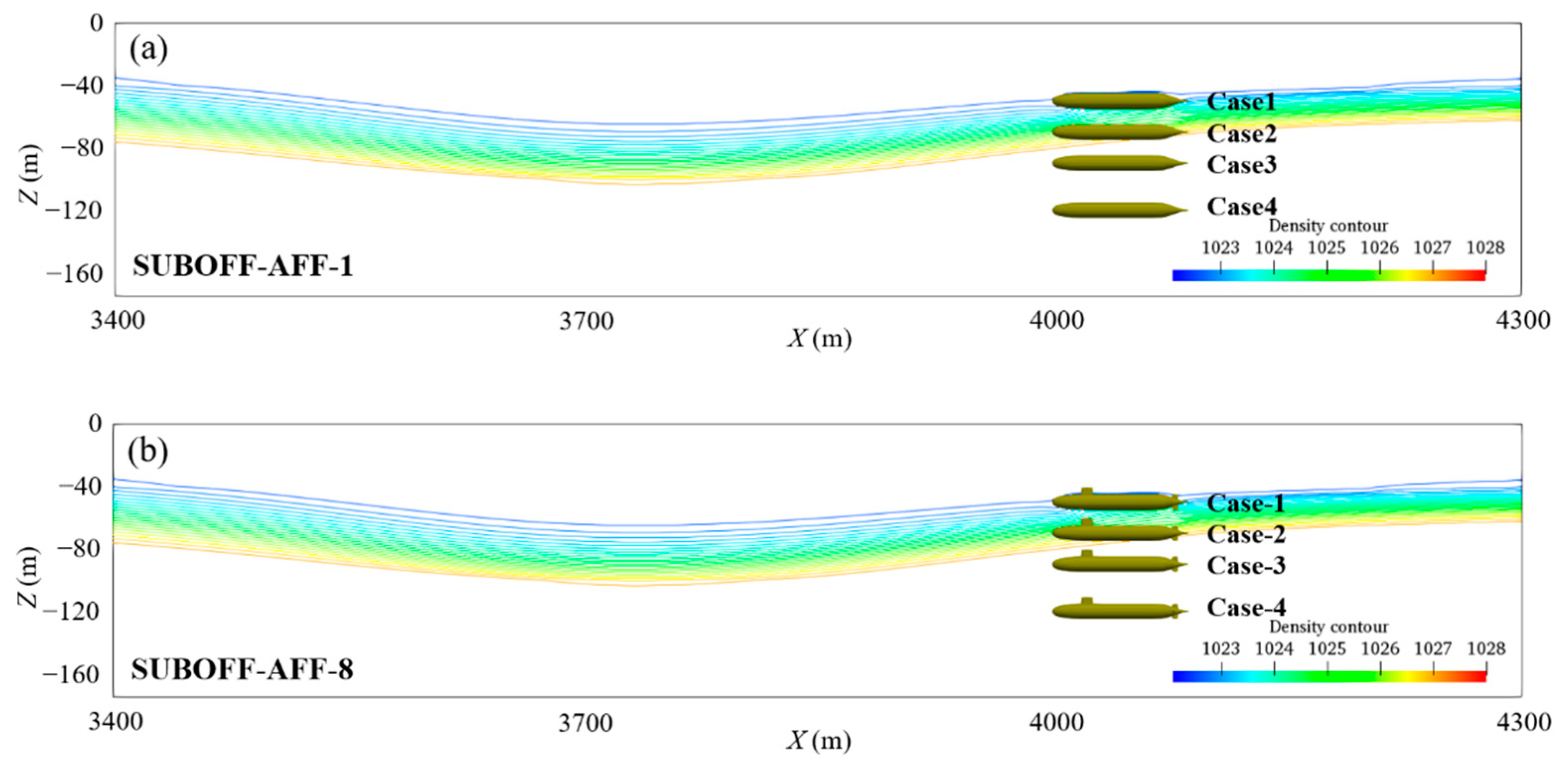
4.1. Computational Domain and Simulation Conditions
4.2. ISW Forces Analysis
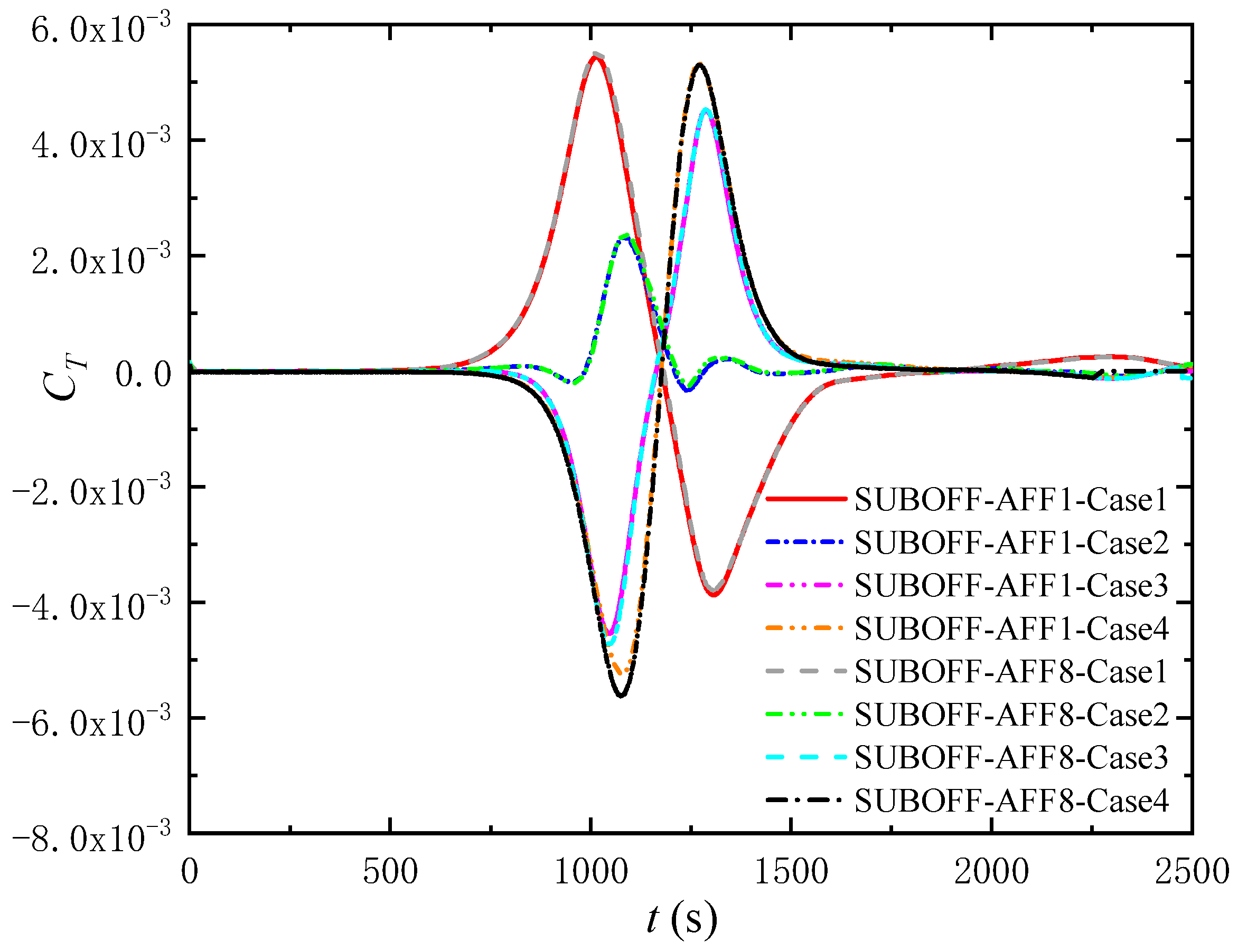
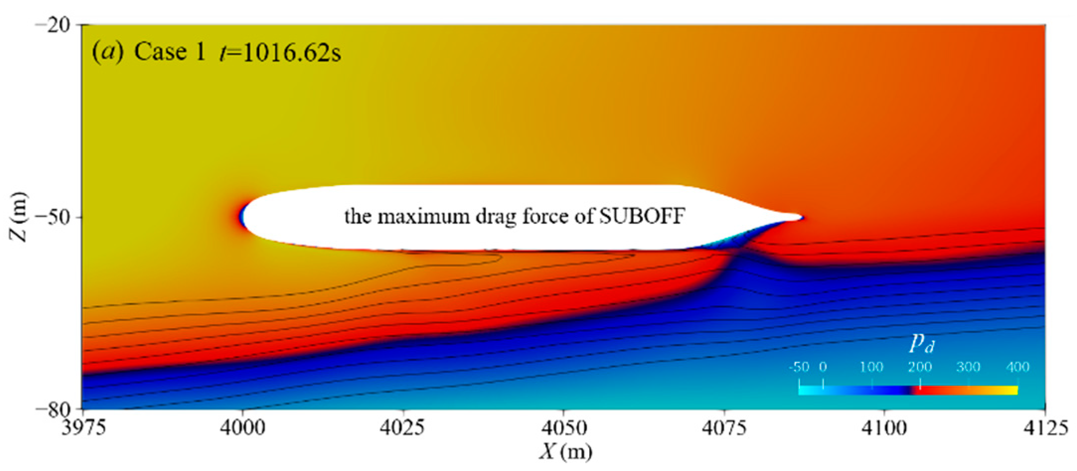
4.2.1. Drag Force
4.2.2. Lift Force
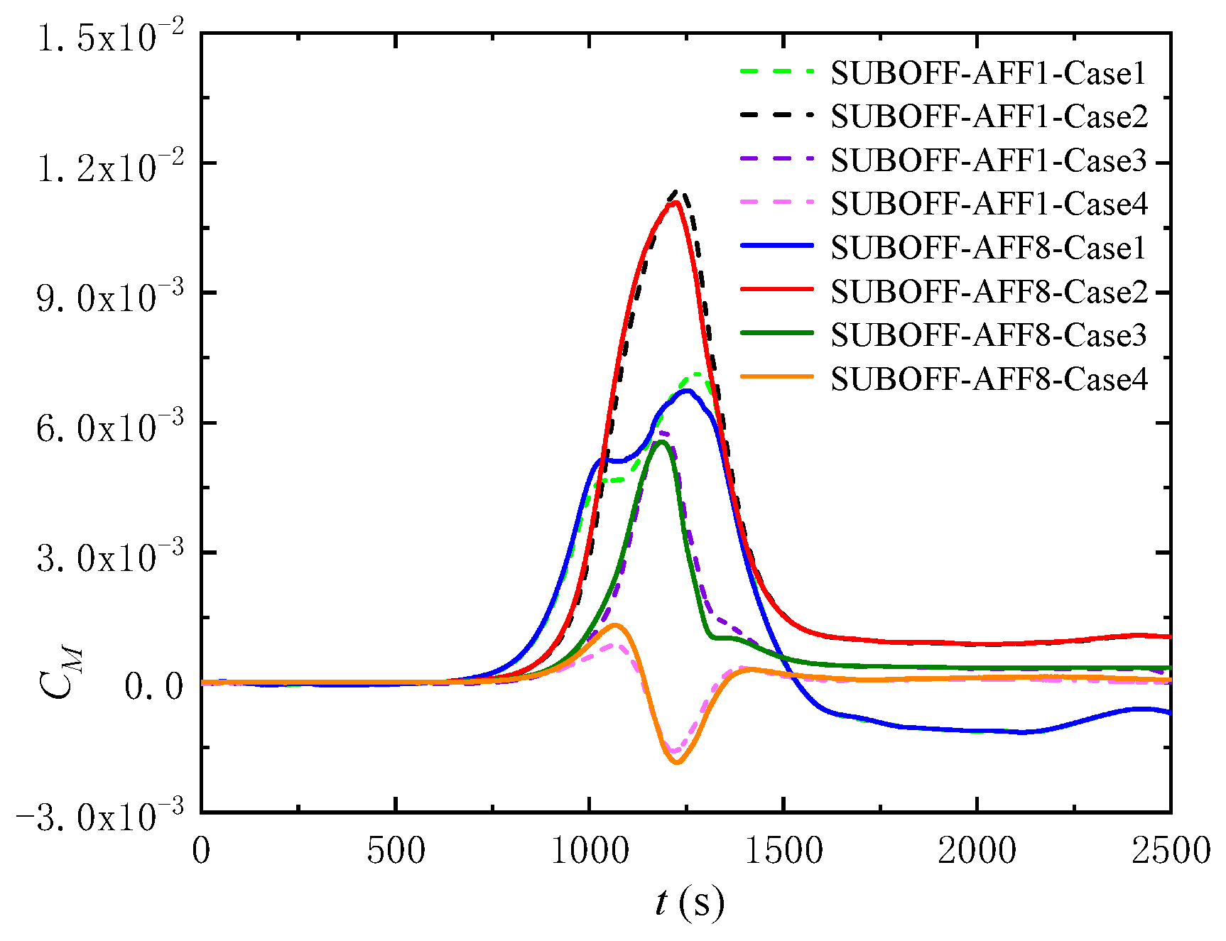
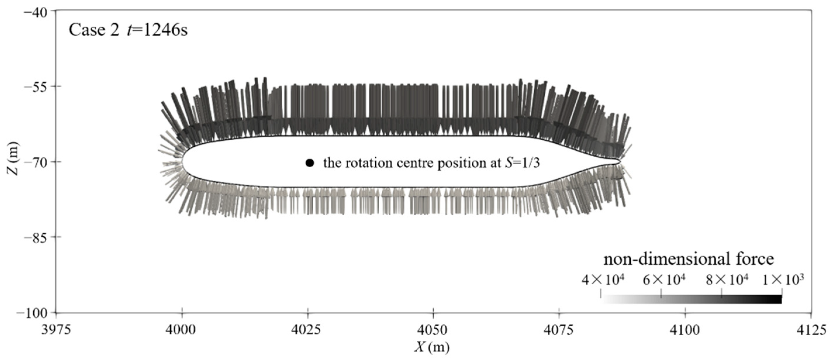
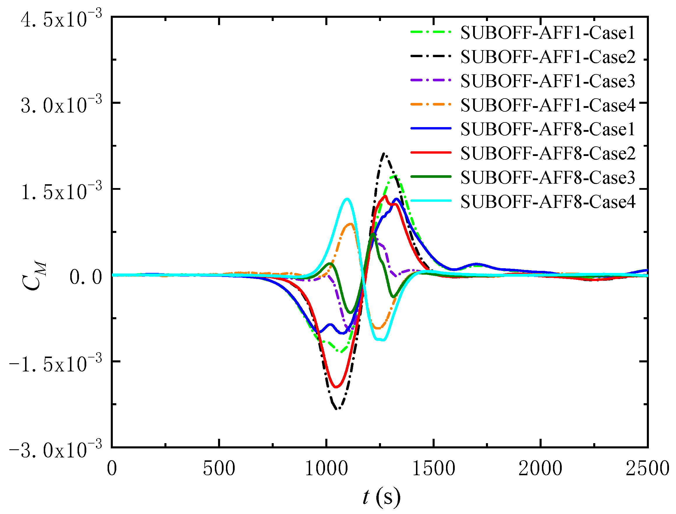
4.2.3. Moment
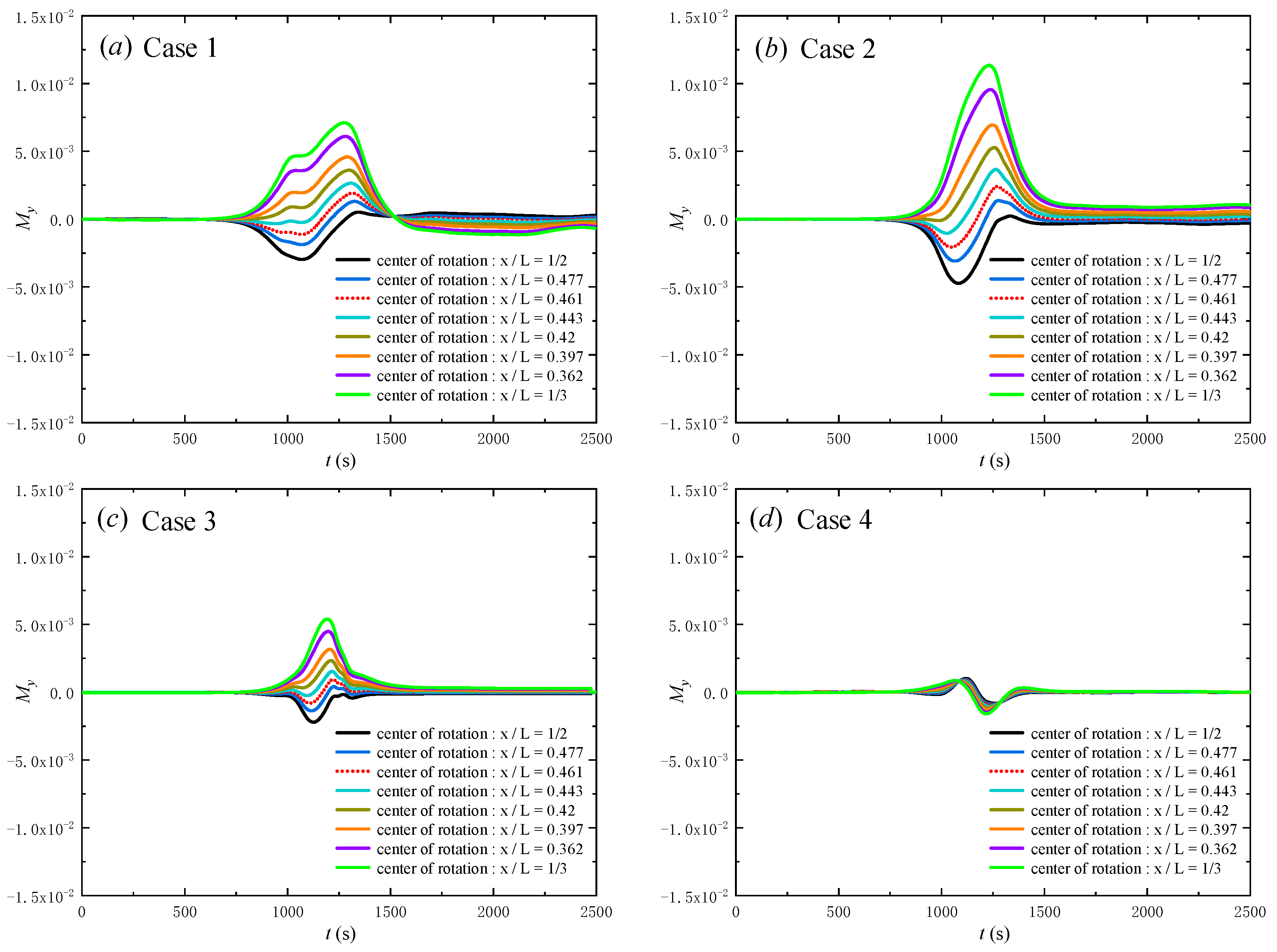
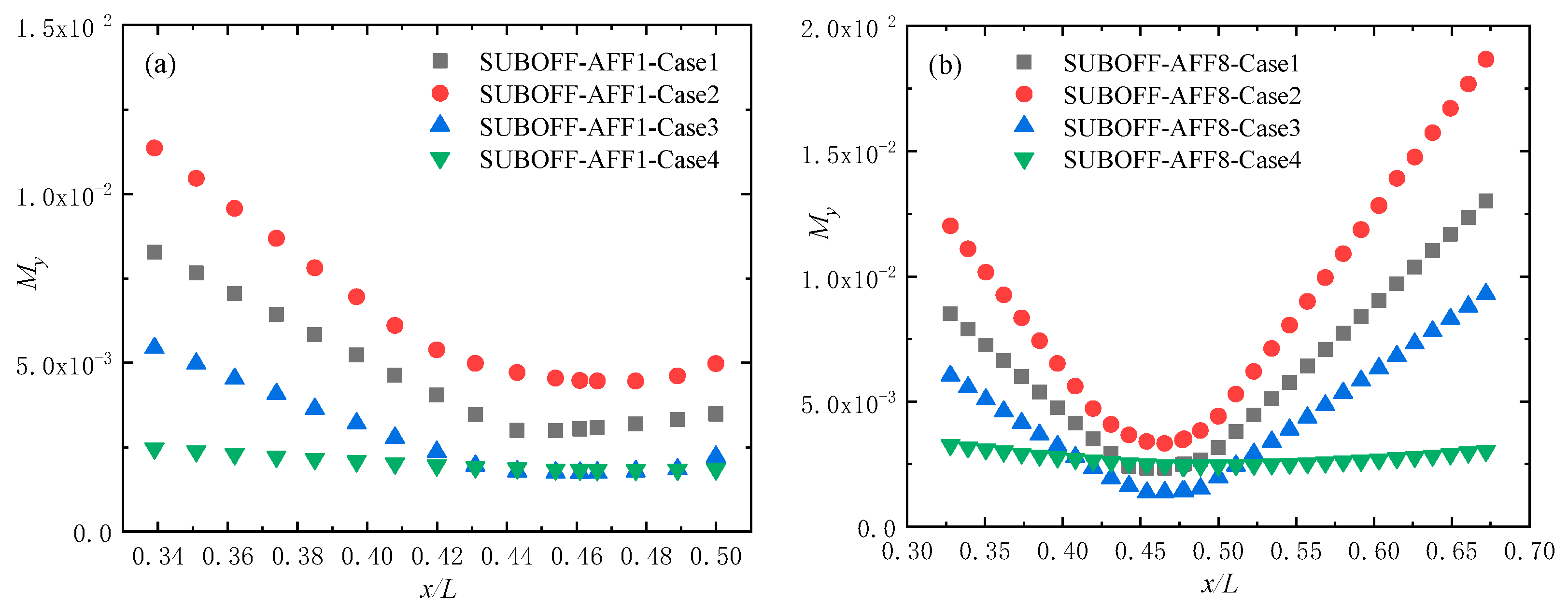
4.3. Effects of the Rotation Centre on Momentum
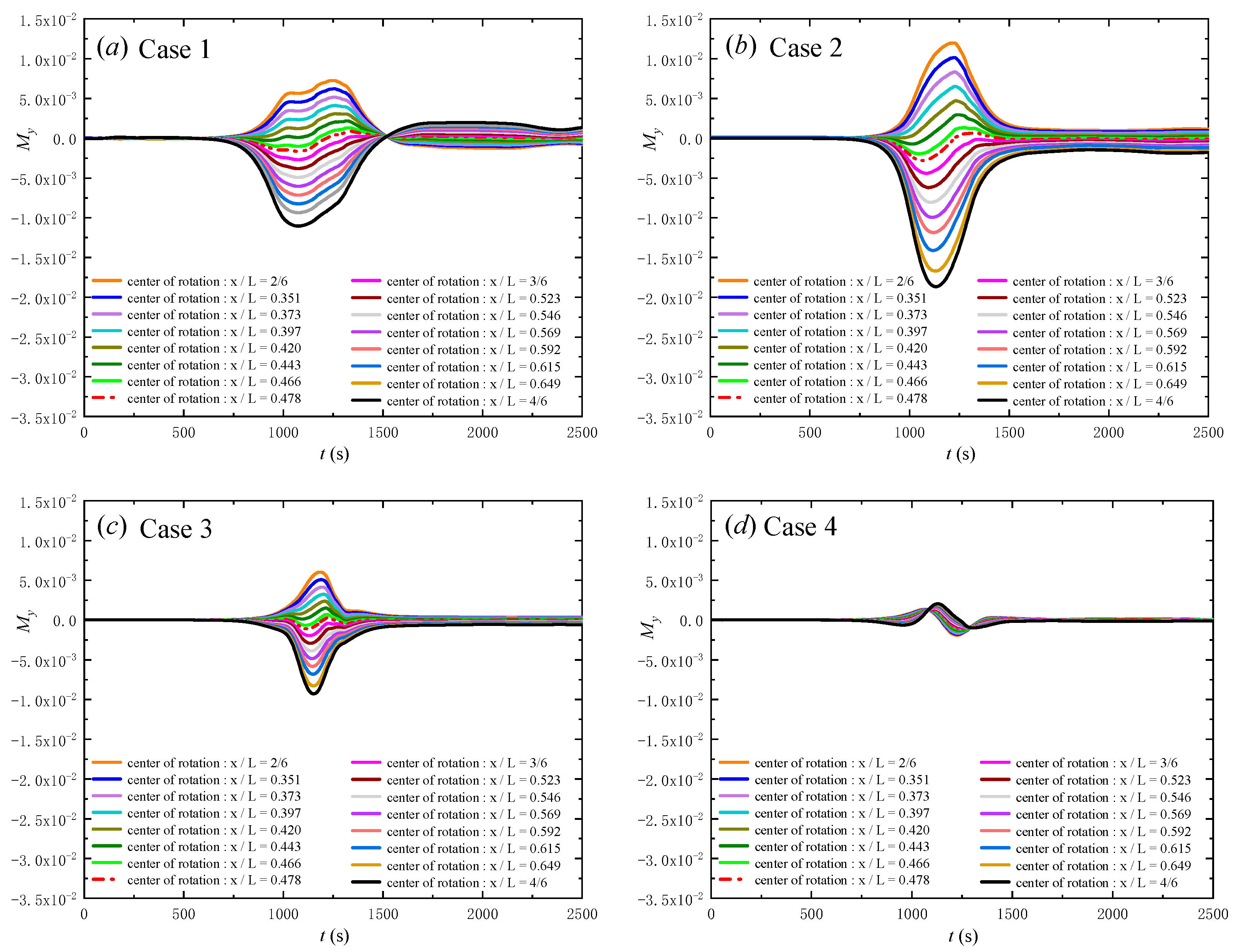
4.4. Analysis of the Optimal Rotation Centre Position
5. Conclusions
Author Contributions
Funding
Institutional Review Board Statement
Informed Consent Statement
Data Availability Statement
Conflicts of Interest
References
- Cai, S.; Xie, J.; He, J. An Overview of Internal Solitary Waves in the South China Sea. Surv. Geophys. 2012, 33, 927–943. [Google Scholar] [CrossRef]
- Lien, R.-C.; Henyey, F.; Ma, B.; Yang, Y.-J. Large-Amplitude Internal Solitary Waves Observed in the Northern South China Sea: Properties and Energetics. J. Phys. Oceanogr. 2014, 44, 1095–1115. [Google Scholar] [CrossRef]
- Dong, J.; Zhao, W.; Chen, H.; Meng, Z.; Shi, X.; Tian, J. Asymmetry of internal waves and its effects on the ecological environment observed in the northern South China Sea. Deep. Sea Res. Part I Oceanogr. Res. Pap. 2015, 98, 94–101. [Google Scholar] [CrossRef]
- Fan, H.; Li, C.; Wang, Z.; Xu, L.; Wang, Y.; Feng, X. Dynamic analysis of a hang-off drilling riser considering internal solitary wave and vessel motion. J. Nat. Gas Sci. Eng. 2017, 37, 512–522. [Google Scholar] [CrossRef] [Green Version]
- Cai, S.; He, J.; Xie, J. Recent Decadal Progress of the Study on Internal Solitons in the South China Sea. Adv. Earth Sci. 2011, 26, 703–710. [Google Scholar]
- Song, Z.J.; Gou, Y.; Teng, B.; Shi, Z.M.; Qu, Y.; Xiao, Y. The motion responses of a Spar platform under internal solitary wave. Acta Oceanol. Sin. 2010, 32, 12–19. [Google Scholar]
- Gong, Y.; Xie, J.; Xu, J.; Chen, Z.; He, Y.; Cai, S. Oceanic internal solitary waves at the Indonesian submarine wreckage site. Acta Oceanol. Sin. 2021, 1, 1–5. [Google Scholar] [CrossRef]
- Groves, N.C.; Huang, T.T.; Chang, M.S. Geometric Characteristics of DARPA Suboff Models:(DTRC Model Nos. 5470 and 5471); David Taylor Research Center: Bethesda, MD, USA, 1989. [Google Scholar]
- Fu, D.M.; You, Y.X.; Li, W. Numerical simulation of internal solitary waves with a submerged body in a two-layer fluid. Ocean. Eng. 2009, 37, 38–44. (In Chinese) [Google Scholar]
- Chen, J.; You, Y.X.; Liu, X.; Wu, C. Numerical simulation of interaction of internal solitary waves with a moving submarine. Chin. J. Hydrodyn. 2010, 25, 344–350. [Google Scholar]
- Guan, H.; Wei, G.; Du, H. Hydrodynamic properties of interactions of three-dimensional internal solitary waves with submarine. J. PLA Univ. Sci. Technol. Nat. Sci. Ed. 2012, 13, 277–582. (In Chinese) [Google Scholar]
- Huang, M.M.; Zhang, N.; Zhu, A. Numerical simulation of the interaction motion features for a submarine with internal solitary wave. In Proceedings of the 30th International Ocean and Polar Engineering Conference, OnePetro, Shanghai, China, 11–16 October 2020; pp. 1805–1812. [Google Scholar]
- Orr, M.H.; Mignerey, P.C. Nonlinear internal waves in the South China Sea: Observation of the conversion of depression internal waves to elevation internal waves. J. Geophys. Res. Space Phys. 2003, 108, 3064. [Google Scholar] [CrossRef]
- Alford, M.H.; Lien, R.-C.; Simmons, H.; Klymak, J.; Ramp, S.; Yang, Y.-J.; Tang, D.; Chang, M.-H. Speed and Evolution of Nonlinear Internal Waves Transiting the South China Sea. J. Phys. Oceanogr. 2010, 40, 1338–1355. [Google Scholar] [CrossRef]
- Kirby, J.T.; Wei, G.; Chen, Q.; Kennedy, A.B.; Dalrymple, R.A. Fully Nonlinear Boussinesq Wave Model Documentation and User’s Manual; Research Rep. CACR-98-06; Center for Appl. Coastal Res., University of Delaware: Newark, DE, USA, 1998. [Google Scholar]
- Small, R.J.; Hornby, R.P. A comparison of weakly and fully non-linear models of the shoaling of a solitary internal wave. Ocean Model. 2005, 8, 395–416. [Google Scholar] [CrossRef]
- Devolder, B.; Troch, P.; Rauwoens, P. Performance of a buoyancy-modified k-ω and k-ω SST turbulence model for simulating wave breaking under regular waves using OpenFOAM®. Coast. Eng. 2018, 138, 49–65. [Google Scholar] [CrossRef] [Green Version]
- Wilcox, D.C. Comparison of two-equation turbulence models for boundary layers with pressure gradient. AIAA J. 1993, 31, 1414–1421. [Google Scholar] [CrossRef]
- Bardina, J.; Huang, P.; Coakley, T. Turbulence modeling validation. NASA Tech. Memo. 1997, 110446, 147. [Google Scholar] [CrossRef]
- Menter, F.R.; Kuntz, M.; Langtry, R. Ten years of industrial experience with the SST turbulence model. Turbul. Heat Mass Transfer. 2003, 4, 625–632. [Google Scholar]
- Devolder, B.; Schmitt, P.; Rauwoens, P.; Elsaesser, B.; Troch, P. A review of the implicit motion solver algorithm in OpenFOAM® to simulate a heaving buoy. In Proceedings of the 18th Numerical Towing Tank Symposium. NuTTS, Marstrand, Sweden, 28–30 September 2015. [Google Scholar]
- Issa, R.I. Solution of the implicitly discretised fluid flow equations by operator-splitting. J. Comput. Phys. 1986, 62, 40–65. [Google Scholar] [CrossRef]
- Patankar, S.V. Numerical Heat Transfer and Fluid Flow; CRC Press: Boca Raton, FL, USA, 1980; ISBN 9781315275130. [Google Scholar]
- Long, R.R. On the Boussinesq approximation and its role in the theory of internal waves. Tellus 1965, 17, 46–52. [Google Scholar] [CrossRef] [Green Version]
- Lamb, K.G.; Wan, B. Conjugate flows and flat solitary waves for a continuously stratified fluid. Phys. Fluids 1998, 10, 2061–2079. [Google Scholar] [CrossRef]
- Dunphy, M.; Subich, C.; Stastna, M. Spectral methods for internal waves: Indistinguishable density profiles and double-humped solitary waves. Nonlinear Process. Geophys. 2011, 18, 351–358. [Google Scholar] [CrossRef]
- Li, J.Y.; Zhang, Q.H.; Chen, T.Q. Numerical Simulation of Internal Solitary Wave in Continuously Stratified Fluid. J. Tianjin Univ. (Sci. Technol.) 2021, 54, 161–170. (In Chinese) [Google Scholar]
- Li, J.; Zhang, Q.; Chen, T. ISWFoam: A numerical model for internal solitary wave simulation in continuously stratified fluids. Geosci. Model Dev. 2021. preprint. [Google Scholar]
- Liu, H.-L.; Huang, T.T. Summary of DARPA Suboff Experimental Program Data; Defense Technical Information Center (DTIC), 1998. Available online: https://scholar.google.com.hk/scholar?hl=zh-CN&as_sdt=0%2C5&q=Summary+of+DARPA+Suboff+Experimental+Program+Data&btnG=#d=gs_cit&u=%2Fscholar%3Fq%3Dinfo%3AF1n5CRiuBnUJ%3Ascholar.google.com%2F%26output%3Dcite%26scirp%3D0%26hl%3Dzh-CN (accessed on 27 November 2021).
- Ferziger, J.H.; Peric, M. Computational Methods for Fluid Dynamics; Springer: Berlin, Germany, 1997. [Google Scholar]
- Yang, C.; Lohner, R. Prediction of Flows Over an Axisymmetric Body with Appendages. In The 8th International Conference on Numerical Ship Hydrodynamics; Springer: Busan, Korea, 2003; pp. 147–160. [Google Scholar]
- Sezen, S.; Dogrul, A.; Delen, C.; Bal, S. Investigation of self-propulsion of DARPA Suboff by RANS method. Ocean Eng. 2018, 150, 258–271. [Google Scholar] [CrossRef]
- Alin, N.; Bensow, R.; Fureby, C.; Huuva, T.; Svennberg, U. Current Capabilities of DES and LES for Submarines at Straight Course. J. Ship Res. 2010, 54, 184–196. [Google Scholar] [CrossRef]


| Φ | σk | σω | Cβ | Cγ |
|---|---|---|---|---|
| Φ1 | 0.85 | 0.5 | 0.075 | 5/9 |
| Φ2 | 1.0 | 0.856 | 0.0828 | 0.44 |
| DARPA SUBOFF | Overall Length (m) | Maximum Diameter (m) | Surface Area (m2) | Submarine Displacement (m3) |
|---|---|---|---|---|
| SUBOFF-AFF-1 | 4.356 | 0.508 | 5.989 | 0.699 |
| SUBOFF-AFF-8 | 4.356 | 0.508 | 6.348 | 0.706 |
| Velocity (m/s) | Numerical Results (N) | Experimental Results (N) | Relative Error (%) |
|---|---|---|---|
| 3.046 | 89.89 | 87.4 | 2.849 |
| 5.144 | 244.03 | 242.2 | 0.756 |
| 6.091 | 329.862 | 332.9 | −0.913 |
| 7.161 | 443.578 | 451.5 | −1.755 |
| 8.231 | 571.378 | 576.9 | −0.957 |
| 9.255 | 708.548 | 697 | 1.657 |
| Velocity (m/s) | Numerical Results (N) | Experimental Results (N) | Relative Error (%) |
|---|---|---|---|
| 3.051 | 103.18 | 102.3 | 0.860 |
| 5.144 | 269.37 | 283.8 | −5.085 |
| 6.096 | 367.42 | 389.2 | −5.596 |
| 7.161 | 495.866 | 526.6 | −5.836 |
| 8.231 | 644.206 | 675.6 | −4.647 |
| 9.255 | 787.332 | 821.1 | −4.113 |
| SUBOFF | S(x/Ls) | |||||||
|---|---|---|---|---|---|---|---|---|
| SUBOFF-AFF-1 | 1/3 | 0.351 | 0.362 | 0.374 | 0.385 | 0.397 | 0.408 | 0.420 |
| 0.431 | 0.443 | 0.454 | 0.461 | 0.466 | 0.477 | 0.489 | 1/2 | |
| SUBOFF-AFF-8 | 2/6 | 0.351 | 0.362 | 0.374 | 0.385 | 0.397 | 0.408 | 0.42 |
| 0.431 | 0.443 | 0.454 | 0.466 | 0.478 | 0.489 | 3/6 | 0.511 | |
| 0.523 | 0.534 | 0.546 | 0.557 | 0.569 | 0.58 | 0.592 | 0.603 | |
| 0.615 | 0.626 | 0.638 | 0.649 | 0.661 | 4/6 | |||
Publisher’s Note: MDPI stays neutral with regard to jurisdictional claims in published maps and institutional affiliations. |
© 2021 by the authors. Licensee MDPI, Basel, Switzerland. This article is an open access article distributed under the terms and conditions of the Creative Commons Attribution (CC BY) license (https://creativecommons.org/licenses/by/4.0/).
Share and Cite
Li, J.; Zhang, Q.; Chen, T. Numerical Investigation of Internal Solitary Wave Forces on Submarines in Continuously Stratified Fluids. J. Mar. Sci. Eng. 2021, 9, 1374. https://doi.org/10.3390/jmse9121374
Li J, Zhang Q, Chen T. Numerical Investigation of Internal Solitary Wave Forces on Submarines in Continuously Stratified Fluids. Journal of Marine Science and Engineering. 2021; 9(12):1374. https://doi.org/10.3390/jmse9121374
Chicago/Turabian StyleLi, Jingyuan, Qinghe Zhang, and Tongqing Chen. 2021. "Numerical Investigation of Internal Solitary Wave Forces on Submarines in Continuously Stratified Fluids" Journal of Marine Science and Engineering 9, no. 12: 1374. https://doi.org/10.3390/jmse9121374
APA StyleLi, J., Zhang, Q., & Chen, T. (2021). Numerical Investigation of Internal Solitary Wave Forces on Submarines in Continuously Stratified Fluids. Journal of Marine Science and Engineering, 9(12), 1374. https://doi.org/10.3390/jmse9121374