Article

Surface Chlorophyll-A Fronts in the Yellow and Bohai Seas Based on Satellite Data

1
College of Earth Science and Engineering, Shandong University of Science and Technology, Qingdao 266590, China
2
College of Ocean Science and Engineering, Shandong University of Science and Technology, Qingdao 266590, China
3
State Key Laboratory of Estuarine and Coastal Research, East China Normal University, Shanghai 200241, China
4
Key Laboratory of Coastal Zone Environmental Processes and Ecological Remediation, Yantai Institute of Coastal Zone Research, Chinese Academy of Sciences, Yantai 264003, China
*
Author to whom correspondence should be addressed.
J. Mar. Sci. Eng. 2021, 9(11), 1301; https://doi.org/10.3390/jmse9111301
Submission received: 9 October 2021 / Revised: 7 November 2021 / Accepted: 18 November 2021 / Published: 20 November 2021
(This article belongs to the Special Issue Satellite Monitoring of Ocean)

Abstract

:
Chlorophyll fronts are important to monitor and map the oceanic front, especially in the season when sea surface temperature (SST) fronts weaken. In this study, surface chlorophyll-a (chl-a) fronts in the Yellow and Bohai seas were characterized for the first time using satellite data. Five distinct chl-a fronts (i.e., the Bohai Strait, Shandong Peninsula, Jiangsu, Liaodong Peninsula, and Korean Peninsula fronts) were observed in summer along the 40 m isobaths and faded in other seasons. Notably, these fronts coincided with SST fronts. Strong chl-a fronts emerged during summer due to chl-a blooms in eutrophic coastal waters paired with surface chl-a fading in strongly stratified offshore waters and coastal physical fronts. Although SST fronts were strong during winter, light limitation and strong vertical mixing in offshore waters led to low chl-a in both coastal and offshore waters, suppressing chl-a front formation. Both chl-a and SST fronts coincided with steep seabed slopes (slope ratio > 1), suggesting that seabed slope may be an indicator of oceanic front location.

1. Introduction

An oceanic front is a narrow zone of intensified horizontal gradients of water properties (i.e., physical, chemical, or biological) that separates different water masses (e.g., [1,2]). Fronts are a common marine phenomenon occurring in coastal, shelf, and pelagic waters, and play an important role in hydrodynamics and the transport of heat, salt, and nutrients, influencing ecological processes, sedimentation, and ocean-atmosphere interaction (e.g., [2,3,4,5]).
Sea surface temperature (SST) fronts are common and widely-studied physical fronts (e.g., [6,7]). Lateral gradients can also be detected in surface chlorophyll-a (chl-a) concentration, which serves as a proxy for phytoplankton biomass [8]. Chl-a can act as a passive tracer of physical dynamics and can be used to estimate productivity (e.g., [9,10]). Thus, chl-a fronts are often used to represent biological fronts, which can be defined as transition regions that separate high-productivity from low-productivity waters and establish the boundaries between different nutrient concentrations. For instance, the basin-wide chl-a front in the mid-latitude North Pacific clearly separates the low-surface chl-a subtropical gyre from the high-surface chl-a subarctic gyre [11]. Chl-a fronts are also important to monitor and map the oceanic front, especially in the summer season when the SST front weakens or disappears [2]. For instance, Legeckis et al. (2002) used the SeaWiFS chl-a to map the Loop Current Front in summer to cover gaps in the GOES SST dataset [12]. Based on surface chl-a data, Hu et al. (2003) studied front formation mechanisms around Hainan Island, northwest of the South China Sea [13]. Additionally, some oceanic front zones feature biological aggregation and strong physical and environmental variability. The relationship between chl-a fronts and SST fronts can reflect the effect of physical processes on the chemical and biological process, which is of spatio-temporal variability and complex (e.g., [2,14]). Therefore, more research is required to better understand the relationship between chl-a fronts and physical fronts [2].
The Bohai and Yellow seas, located north of the East China Sea, are representative semi-enclosed shelf seas, connected with each other through the Bohai Strait (Figure 1a). The mean depth of the Bohai Sea is approximately 20 m; the Yellow Sea is surrounded by China and the Korean Peninsula, and has a mean depth of approximately 44 m. The shallow Bohai Sea is highly influenced by tidal motion, which plays a predominant role in water renewal (e.g., [15]). Moreover, the water residence time of the Bohai Sea exceeds two years and exhibits a weak water exchange with the Yellow Sea due to its relatively narrow shorelines [16]. Unlike the Bohai Sea, the Yellow Sea exhibits substantially distinct seasonal hydrodynamics. In winter, the prevailing southern cool currents forced by the northerly East Asian monsoon wind occur along both China and the Korean Peninsula coasts, while a compensated warm current (i.e., the Yellow Sea Warm Current) flows north along the central trough of the Yellow Sea (Figure 1b) [17,18]. From spring to summer, the Yellow Sea Cool Water Mass in the bottom of the central Yellow Sea gradually forms and, combined with intensified sea surface heating, the stratification in the Yellow Sea offshore becomes the strongest in August [19]; cyclonic circulation also occurs along the Yellow Sea coastal waters (Figure 1c) (e.g., [20]). Many rivers are distributed along the coast of the Bohai and Yellow seas, including the Chang Jiang and the Yellow rivers, which are the rivers with the highest runoff and sediment discharge in China, respectively. These rivers carry vast amounts of sediments and abundant land nutrients along with freshwater into the Bohai and Yellow seas, resulting in high turbidity and nutrient enrichment, especially in coastal waters [21,22,23,24]. Moreover, the Yellow Sea coast exhibits high turbidity (10–50 FTN; i.e., Formazin Turbidity Unit) in winter due to the strong monsoon wind. However, it becomes relatively clear (1–5 FTN) in summer, especially in surface waters [25]. Similar seasonal turbidity variations occur in the Bohai Sea, which has a significant influence on the seasonal variability of chl-a [26].
Several studies on the SST fronts in the Yellow and Bohai seas have been conducted using satellite data (e.g., [6,17,27,28,29]). These studies suggest that strong sea surface cooling and topography act in conjunction with the shear between the cool coastal current and the Yellow Sea warm current to induce strong SST coastal fronts during the winter. In contrast, the tidal front, which separates well-mixed from stratified water, dominates the coastal fronts during summer. These SST fronts have been abundantly studied; however, there is hardly any research regarding chl-a fronts in the highly turbid and eutrophicated Yellow and Bohai seas. Moreover, the relationship between the SST and chl-a fronts in the Yellow and Bohai seas are poorly understood. In this study, a well-validated chl-a dataset derived from MODIS (i.e., moderate resolution imaging spectroradiometer) satellite data was used to diagnose chl-a fronts in the Bohai and Yellow seas, and the spatial pattern and seasonal variability of five chl-a fronts were characterized for the first time. Moreover, our study discusses the formation of chl-a fronts and their relationship with SST fronts.

2. Materials and Methods

2.1. Chl-a and SST Satellite Data

Chl-a concentration satellite data were obtained from Wang et al. (2017) [30], who compared and developed algorithms to estimate chl-a concentration from MODIS data in the Yellow and Bohai seas (hereafter referred to as “YB sea”). To address large biases in conventional algorithms (i.e., OC3M, ocean chlorophyll-a three-band algorithm for MODIS and GSM01, Graver–Siegel–Maritorena model version 1 algorithm), Wang et al. (2017) developed a generalized additive model (GAM) and improved the accuracy of satellite-derived chl-a data in the YB sea [30]. The MODIS-aqua Level 2 daily remote-sensing reflectance (Rrs) images from June 2002 to December 2016 were downloaded from the NASA Goddard Space Flight Center (GSFC, http://oceancolor.gsfc.nasa.gov/cms/, accessed on 15 June 2020). Then, the GAM method was implemented for the retrieval of chl-a concentrations from MODIS Rrs images. Finally, the data retrieval was based on the output of the GAM, to which the MODIS data above water Rrs, in situ measured chl-a concentration, and water depth were inputted. The GAM algorithm could significantly diminish the effect of suspended sediments and colored dissolved organic matter and bottom reflectance in shallow waters by using a water-depth dependent model. The algorithm rendered much better results with the validation of additional in situ measured chl-a data from 5 cruises and more than 400 stations in 2010–2013, exhibiting a mean absolute percentage difference (MAPD) of 39.96% and a coefficient of determination (R2) of 0.67. The MAPD and R2 were calculated from comparisons between satellite and in situ chlorophyll for those pixels where both amounts are available. In contrast, the OC3M and GSM01 algorithms exhibited an MAPD of >110% and R2 of <0.25 [30]. Therefore, the data rendered by the GAM algorithm was considered reliable for this study. More details regarding the GAM algorithm and validation results can be found in [30].
The chl-a data horizontal resolution was 4 km × 4 km, and this study focused on the seasonal characteristics of the chl-a front. Therefore, the data from June 2002 to December 2016 were averaged monthly to obtain monthly chl-a concentrations. The monthly data were then used to characterize the monthly variability of chl-a patterns and fronts.
The nighttime Level 3 mapped SST data from MODIS/Aqua from 2002 to 2016 were used to diagnose SST fronts in the YB sea. Additionally, we checked that the daytime SST data got the same SST-front pattern and intensity with the nighttime SST. These SST datasets with a spatial resolution of 4 km were downloaded from the U.S. National Aeronautics and Space Administration (NASA) website (http://oceancolor.gsfc.nasa.gov, accessed on 15 June 2020). To match the chl-a data, climatological monthly mean SST data were used in this study, which was calculated averaging all data obtained for the entire period during each particular month. The monthly rainfall data in the area around the YB sea (117–129° E, 30–42° N) from 2002 to 2016 were derived from U.S. National Oceanic and Atmospheric Administration (NOAA) (https://psl.noaa.gov/data/gridded/data.cmap.html, accessed on 2 November 2021) and used in the analysis.

2.2. Front Detection

The algorithm for oceanic front detection developed by [2] was used to diagnose the position and magnitude of chl-a and SST fronts in the YB sea. Based on the contextual feature-preserving filter and traditional gradient method, the algorithm was proposed to diminish the effect of data noise from the small- and meso-scale chl-a blooms or patchiness. As demonstrated by [2], the algorithm could efficiently remove the data noise. This algorithm had also been used in other oceanic front studies (e.g., [31,32,33]). The key steps of the front detection algorithm are summarized below.
Pre-processing the data via a contextual median filter (MF) until iterative MF convergence is achieved. In the filtering process, the data remain unchanged if the window center is a significant 5-point extremum in 5 × 5 windows. Otherwise, if the window center is a spike (extremum in 3 × 3 windows), the data will be filtered by a 2D 3 × 3 median filter.
Calculating the gradient magnitude for fronts, the gradient is computed via the Sobel operator consisting of 3 × 3 kernels:
G x = [ 1 0 + 1 2 0 + 2 1 0 + 1 ] A ,   G y = [ + 1 + 2 + 1 0 0 0 1 2 1 ] A
where A is the data from step 1, Gx and Gy are two images which contain approximations for derivates in horizontal and vertical directions, and * is the convolution symbol. Afterward, the gradient magnitude (GM) can be calculated as follows:
G M = G x 2 + G y 2
a more detailed description of the algorithm can be found in [2].
Finally, the magnitude of the SST front (expressed as °C/km) could be derived using GM with a 4-km data grid space. According to [2], the ratios of chl-a values between adjacent pixels were used to quantify the chl-a front magnitude, which was calculated via the GM of log-normalized original chl-a data. Based on the chl-a gradient pattern described in Section 3.2, a ratio of >1.1 was chosen as the defining criterion for chl-a fronts, which denoted that the chl-a concentration increased or decreased more than 10% relative to the adjacent grid cell across the front. The seasonal variability of the fronts were analyzed. The four seasons are defined as: spring (April, May, and June), summer (July, August, and September), fall (October, November, and December), and winter (January, February, and March).

3. Results

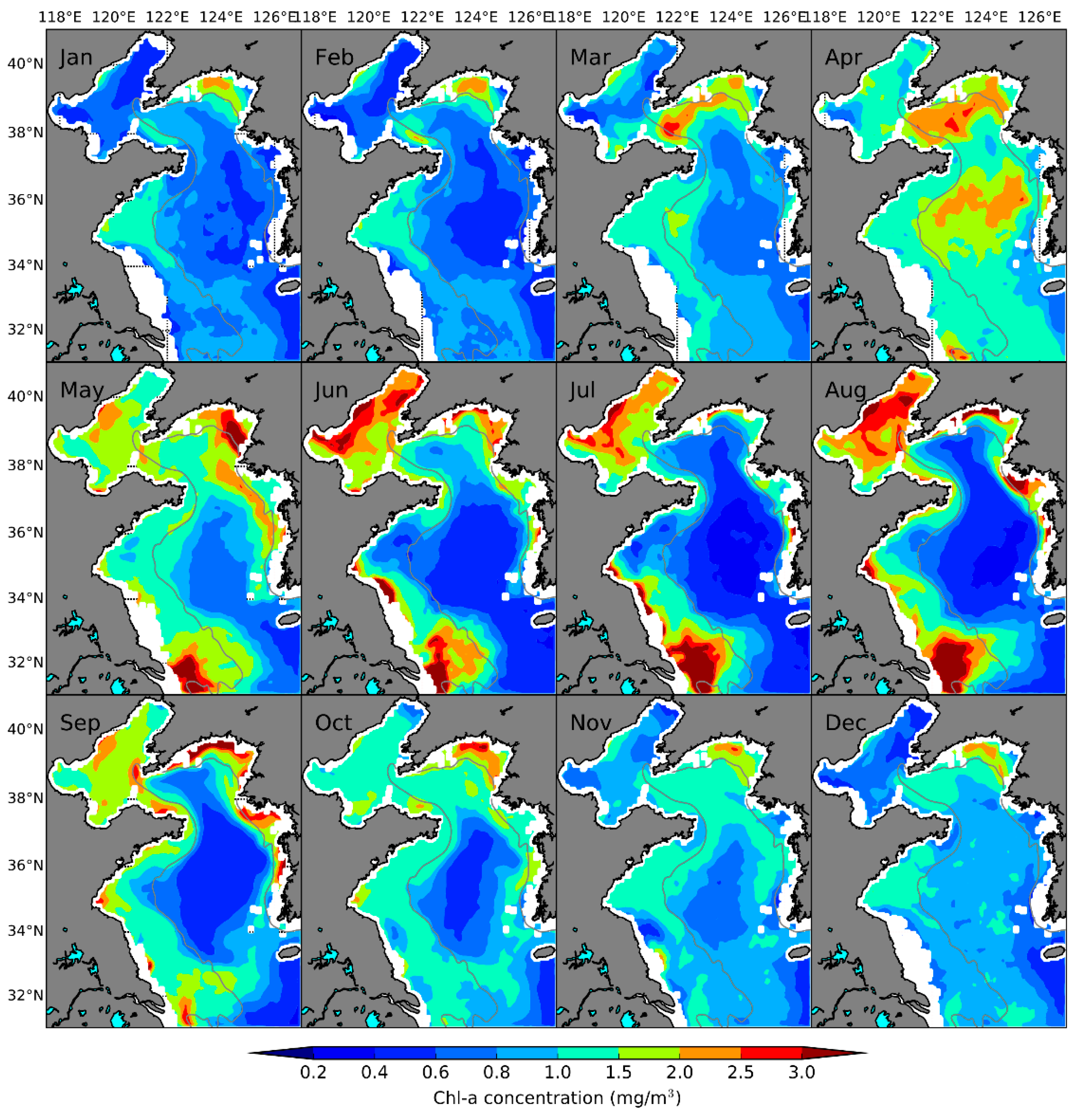
3.1. Satellite-Derived Monthly Chl-a Pattern

Monthly chl-a concentration in the YB sea is illustrated in Figure 2. The coastal chl-a concentration is higher (>1.5 mg/m3) than that offshore from May to October, especially in summer. Moreover, a low-concentration area (<0.6 mg/m3) formed south of the Yellow Sea center, then expanded northwards in July, and descended to the south of the Yellow Sea in October. The boundary between high and low concentrations roughly follows the 40 m isobaths. In autumn and winter, the chl-a concentration is generally low (<1.0 mg/m3) except in the Haizhou Bay and Seohan Bay, and its spatial variability was not significant. In April, the decreasing turbulent kinetic energy and the stratification in the Yellow Sea center induces a relatively high chl-a concentration (>2.0 mg/m3) offshore at depths greater than 40 m, which was consistent with in situ observations (e.g., [34]) and other satellite results (e.g., [35]).
As indicated by [36], topography plays an important role in the seasonal pattern of chl-a in the YB sea, which is consistent with the results discussed above. Therefore, the chl-a in the YB sea was divided into three sections for seasonal variation analysis: the offshore zone (water depth ≥ 40 m), the Yellow Sea coastal zone (water depth < 40 m), and the Bohai Sea. The area of the Bohai Sea with a water depth of <40 m was isolated from the coastal zone due to the fact that it is an enclosed sea and has different hydrodynamic characteristics from those of the relatively open coastal zone along the Yellow Sea coastline. As illustrated in Figure 3, the chl-a concentrations in the offshore zone, the coastal zone, and the Bohai Sea exhibit a notable seasonal variation. In the offshore zone, chl-a exhibits two peaks in spring and autumn, respectively. The chl-a concentration is highest (~1.5 mg/m3) in April due to the spring bloom in the Yellow Sea offshore zone; the other peak (~0.9 mg/m3) in autumn is relatively lower than in spring. The lowest chl-a concentration (~0.5 mg/m3) occurs in summer. The chl-a in the coastal zone exhibits a unimodal variation whereby chl-a is highest in the summer and lowest in the winter. The chl-a variation in the Bohai Sea is similar to that in the Yellow Sea coastal zone, albeit approximately 0.5 mg/m3 higher in summer and 0.3 mg/m3 lower in winter.

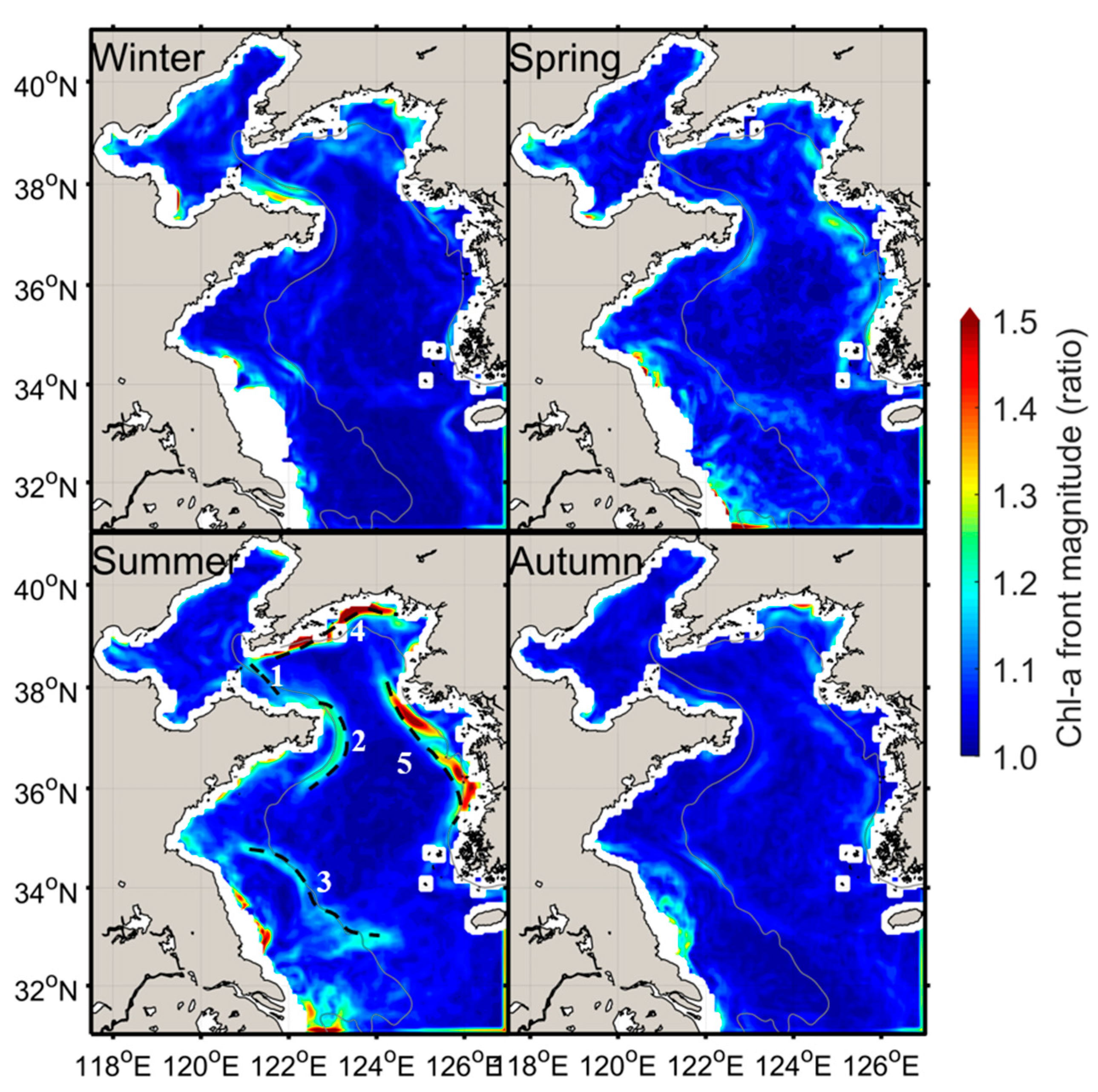
3.2. Chl-a Fronts and Their Seasonal Variation

Figure 4 illustrates the seasonal chl-a front pattern. There are five notable chl-a fronts which manifest stripes denoting a strong chl-a gradient in the Yellow Sea during summer: the Bohai Strait (BS) front, Shandong Peninsula (SP) front, Jiangsu (JS) front, Liaodong Peninsula (LP) front, and Korean Peninsula (KP) front. These five fronts are located near the coast and are largely parallel to the coastline, except for the BS front. The location of the fronts also corresponds to those of the SST fronts, as determined by [6] and this study (see Section 3.3). The maximum magnitude of the five fronts was higher than a 1.2 ratio and even higher than 1.5 in the LP and KP fronts. However, there are no distinct chl-a fronts in other seasons (i.e., other than summer), only small regions north of the Shandong Peninsula and in the Korean Peninsula coast in winter. As shown in Figure 5, the interannual variability of the five chl-a fronts is basically smaller than 0.2. Relatively high variability (~0.3) occurs at the offshore water near the Changjiang estuary and the north of the KP front.
The monthly variations of the five fronts’ intensity are illustrated in Figure 6. These variations were calculated by spatially averaging the magnitude of the five aforementioned fronts. All five fronts exhibited a single-peak monthly variation pattern. Moreover, these fronts developed in June and reached their maximum strength in August (LP front and KP front) or September (BS front and SP front), after which they quickly subsided in October. The JS front intensity reached a maximum in July and a slightly decreased from August to September. Although the BS and LD fronts magnitude was slightly higher than a 1.1 ratio in winter, they were considered weak enough to be negligible.

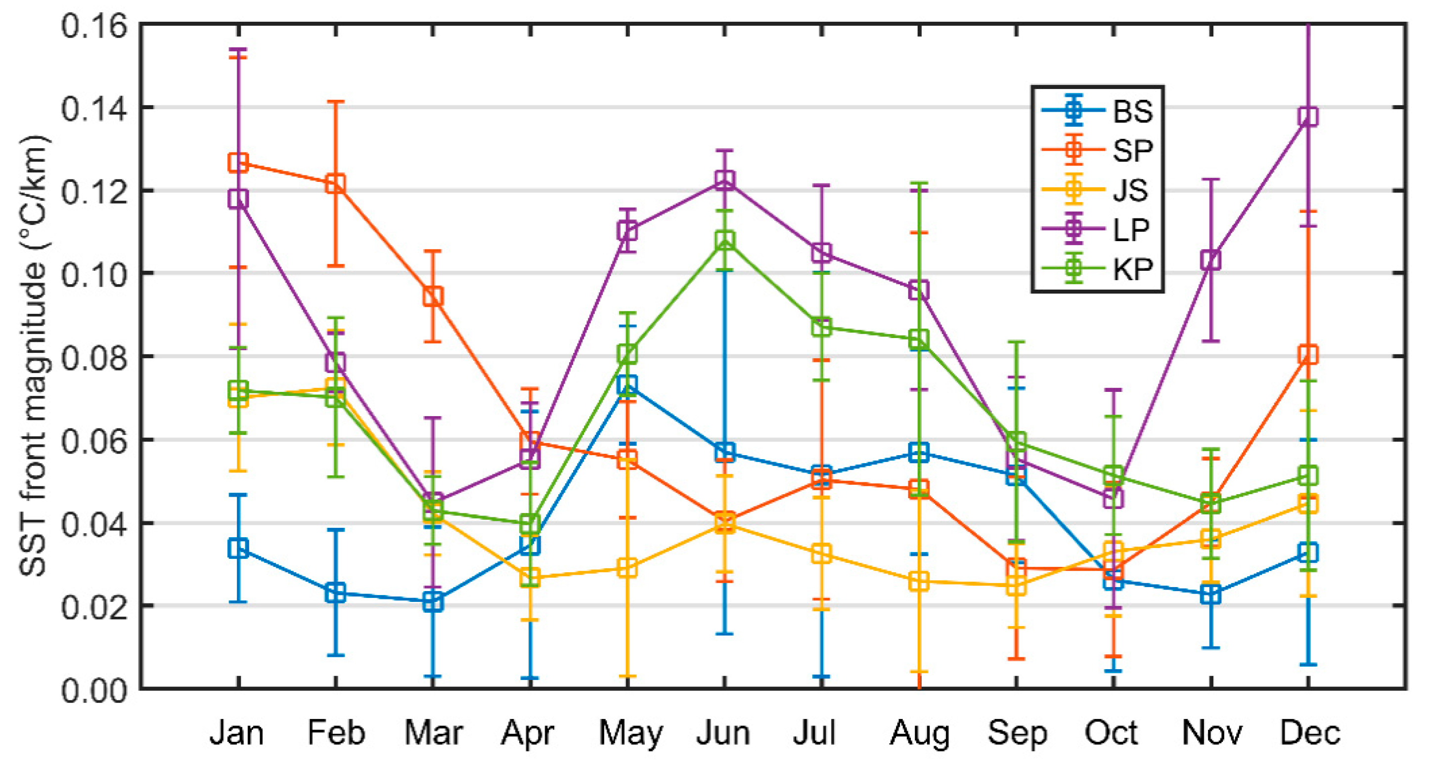
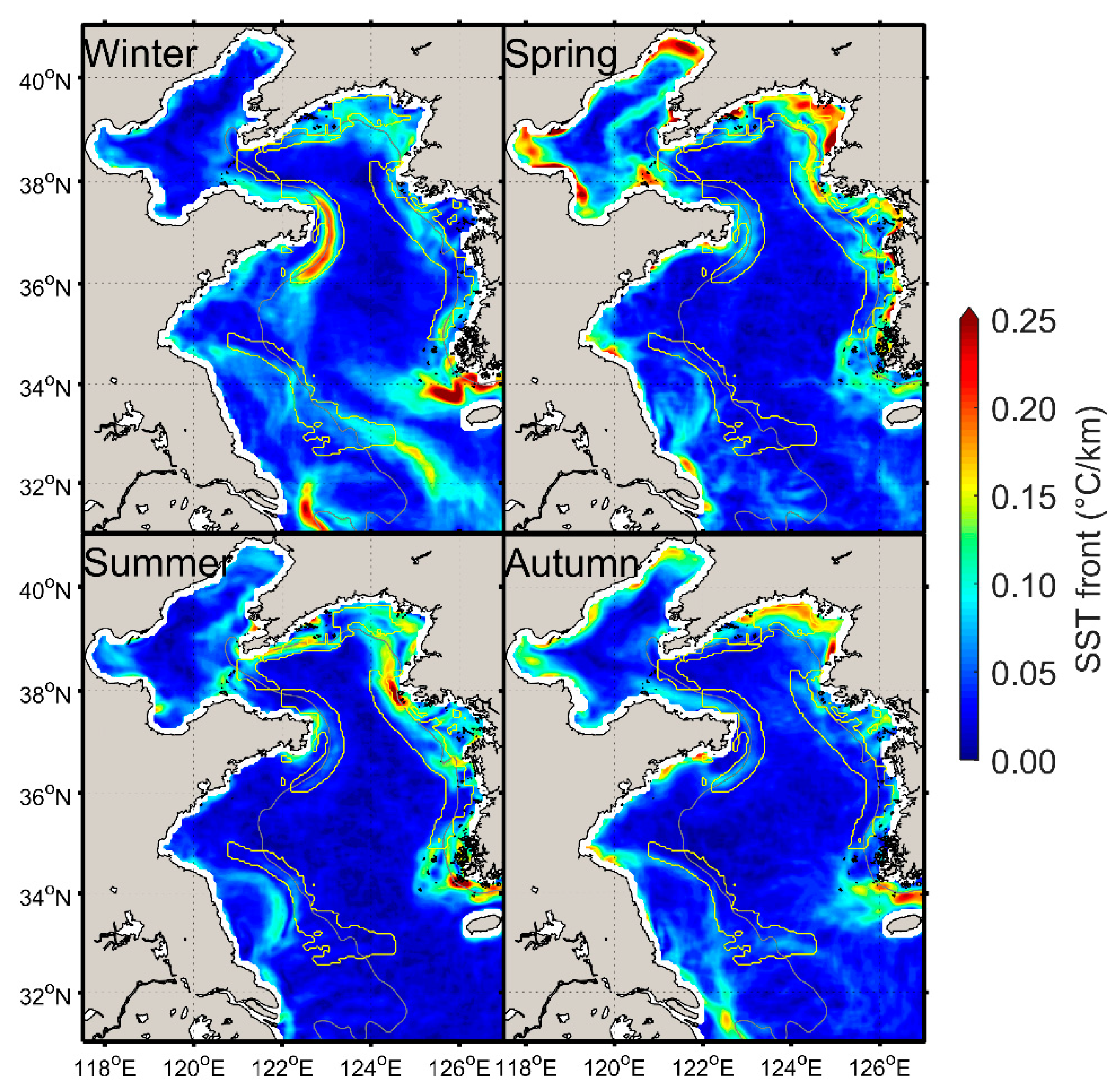
3.3. SST Fronts and Their Seasonal Variation

As illustrated in Figure 7, the SST fronts in the Yellow Sea largely persisted throughout the four seasons. The SST fronts occur in Bohai Strait (BS) and along the Shandong Peninsula (SP), Liaodong Peninsula (LP), Korean Peninsula (KP), and Jiangsu (JS) coastal areas, which is consistent with previous studies (e.g., [6,17,29]). The SST fronts are relatively strong in winter, especially in the Yellow Sea western coasts, and are weak in autumn. In spring and summer, the SP and JS fronts are relatively weak. However, the BS, LP, and KP fronts remain strong.
The location of the SST fronts basically coincided with that of the chl-a fronts (Figure 7). The SST front magnitudes within the five chl-a front zones were spatially averaged as shown in Figure 8, and two SST front peaks were observed in winter and summer. In January and February, the SST fronts were strong [6], especially in the SP front, which was induced by strong surface cooling and the shear between the coastal cold current and the Yellow Sea warm current (e.g., [17]). However, the SP and JS fronts weakened from March to December. In contrast, the LP and KP fronts increased from May to August; both maximum front magnitudes occurred in June. The five fronts were relatively weak in April, September, and October.

4. Discussion

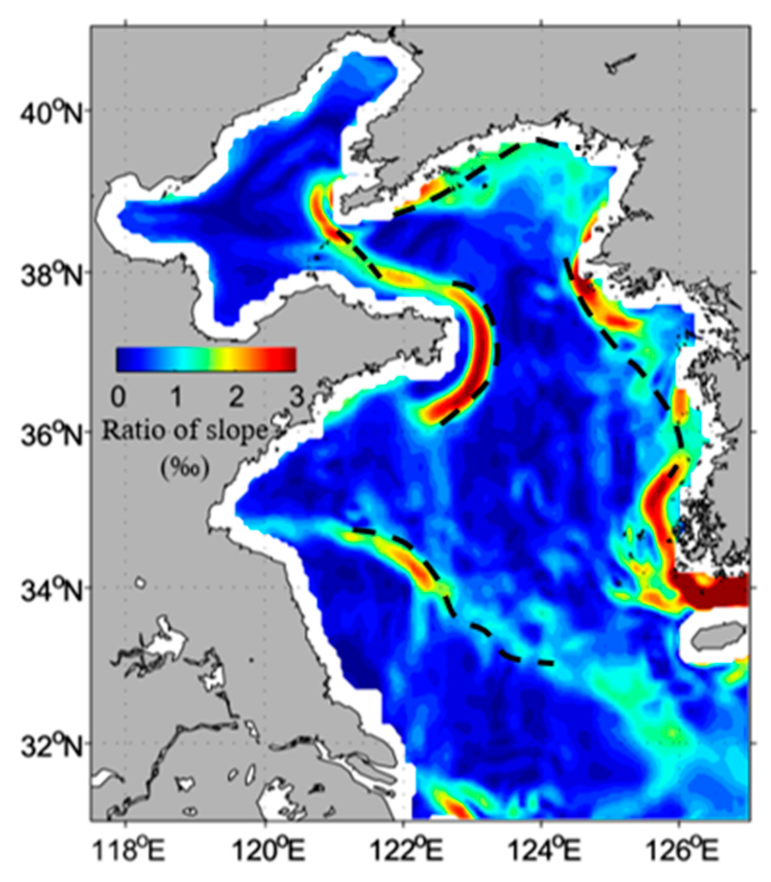
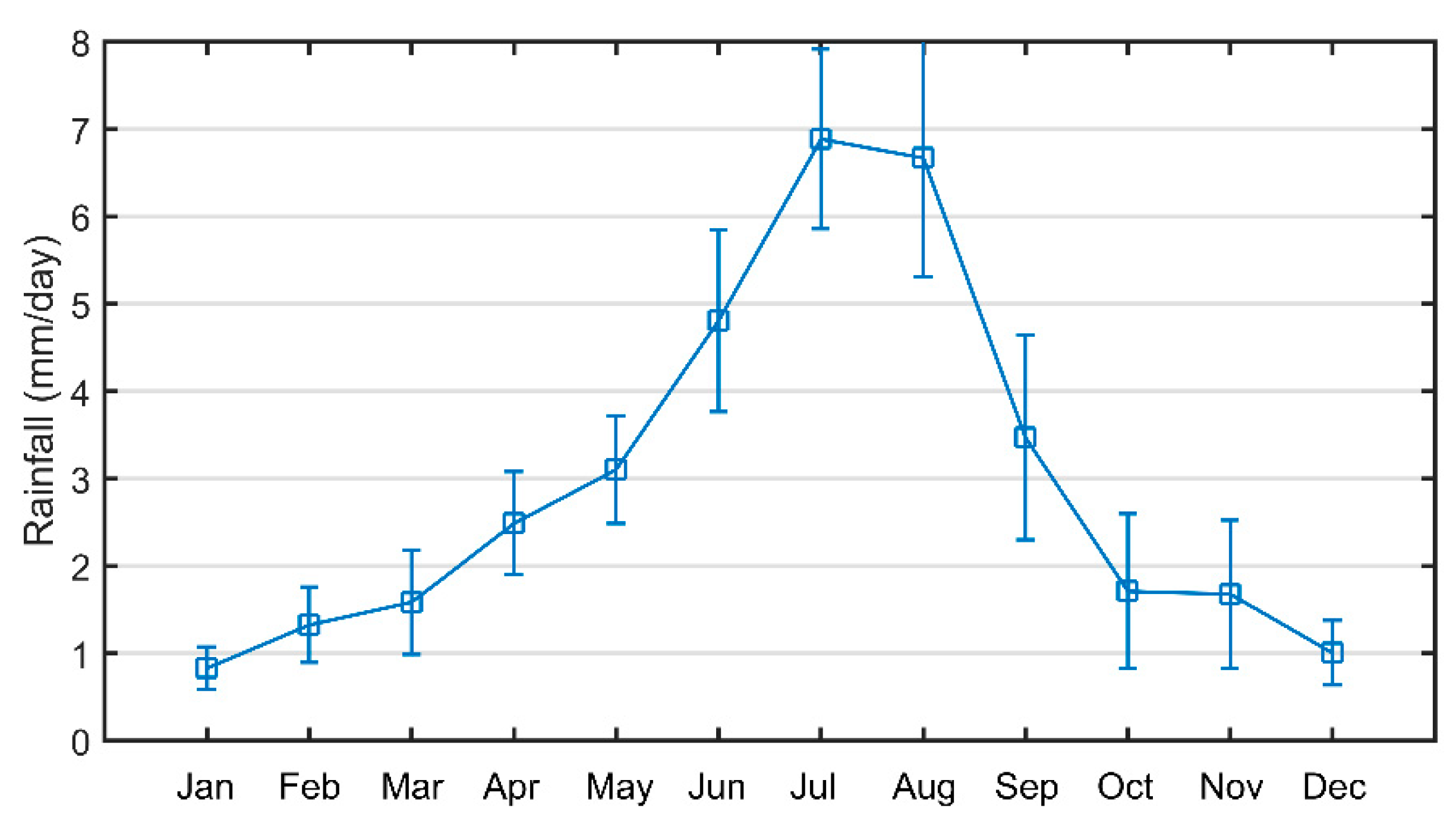
4.1. Interpretation of Signatures of the Chl-a Fronts Based on Physical Oceanography

Several studies have investigated the SST fronts in the YB sea (e.g., [6,17,29]), while this study further investigated the chl-a fronts. It is worth noting that the SST fronts along the LP and KP were referred to as “Seohan Bay front” and “Kyunggi Bay front” by [6], respectively. However, these fronts were referred to as the LP and KP fronts in this study in order to correspond to the chl-a fronts. As shown in Figure 4 and Figure 6, seasonal chl-a fronts exhibited a notable summer unimodal pattern. The fronts were mainly located at the boundary between the shallow onshore water (i.e., including Bohai sea) and the deep offshore water. Overall, the coastal chl-a summer single-peak pattern and the offshore chl-a double-peak pattern observed in spring and autumn (Figure 3) formed the great chl-a gradient in summer and the relatively small ratio in other seasons, which resulted in the observed unimodal pattern of the chl-a fronts in summer.
In summer, the increased runoff during the rainy season carried a substantial amount of terrestrial nutrients into coastal waters (Figure 9) which, in conjunction with sunlight and suitable water temperature, induced algae blooms along most of the Yellow Sea coast and in the semi-enclosed Bohai Sea [36,37]. Meanwhile, the strong stratification of the deep offshore waters limited the replenishment of nutrients from the bottom up, which resulted in low chl-a concertation in the surface under the oligotrophic conditions of the central Yellow Sea (e.g., [34,38]). Coastal blooms and the offshore fading induced strong chl-a fronts in summer. Additionally, the strong tidal fronts emerging in the summer blocked the horizontal exchange of nutrients and chl-a between coastal and offshore waters, which facilitated the formation and persistence of chl-a fronts.
In winter, strong physical fronts and considerable nutrient differences have been observed between the coastal and offshore water (e.g., [39]). Interestingly, no distinct chl-a fronts were observed in winter in the Yellow Sea. The possible underlying mechanisms are discussed below.
In winter, the entire Yellow Sea was vertically well-mixed via intensive surface cooling and strong winds from the Asian monsoon. Moreover, the depth of the mixing layer was approximately equal to the water depth [40]. For the Yellow Sea offshore waters, the nutrient supply to the upper layer was intensified by strong vertical mixing, which should have promoted the growth of phytoplankton in the euphotic layer. However, deep mixing prevented the accumulation of chl-a in the upper layer by transporting the phytoplankton into deep waters, thus weakening photosynthesis and eventually keeping the low chl-a concentrations. On the other hand, high-concentrations of suspended sediment in shallow coastal waters could have been attributable to strong wind, waves, and currents, which induced a thin euphotic layer [41], leading to a decrease in a low chl-a concentration via light limitation [32]. In January and February, the relatively high chl-a concentrations occurring along the Liaodong Peninsula coast (Figure 2) coincided with relatively lower suspended sediment concentrations (SSC) compared with other coastal areas (see Figure 3 in [24]). This observation highlighted the impact of suspended sediments on coastal chl-a concentrations. Therefore, coastal chl-a concentrations decreased under light-limitation, and there was no appreciable distinction between the coastal and offshore chl-a concentrations, which resulted in weak chl-a fronts in winter.
In April, both the weakening wind and increased heating reduced the turbulent energy and increased the stability of the hydrographical structure in the deep waters of the Yellow Sea, which created a suitable hydrodynamic environment for chl-a accumulation in the upper layer and consequently for a spring bloom [35,42]. This spring bloom induced higher concentrations of offshore chl-a, which were even slightly higher than those in the coastal region (Figure 2). The coastal chl-a also increased due to increases in water transparency with the decrease of SSC. Thus, the coastal and offshore chl-a concentrations remained notably similar (Figure 2), and consequently no distinct chl-a fronts were identified. In autumn, the gradual increase in wind and surface cooling disturbed the summer offshore stratification and increased the coastal SSC. This, in turn, induced the offshore increase and coastal decrease for chl-a concentrations, which resulted from the replenishment of nutrients and the decrease of water transparency, respectively. These contrasting variations drove the offshore and coastal chl-a concentration close to each other again, which led to the fading of the summer chl-a front in autumn.

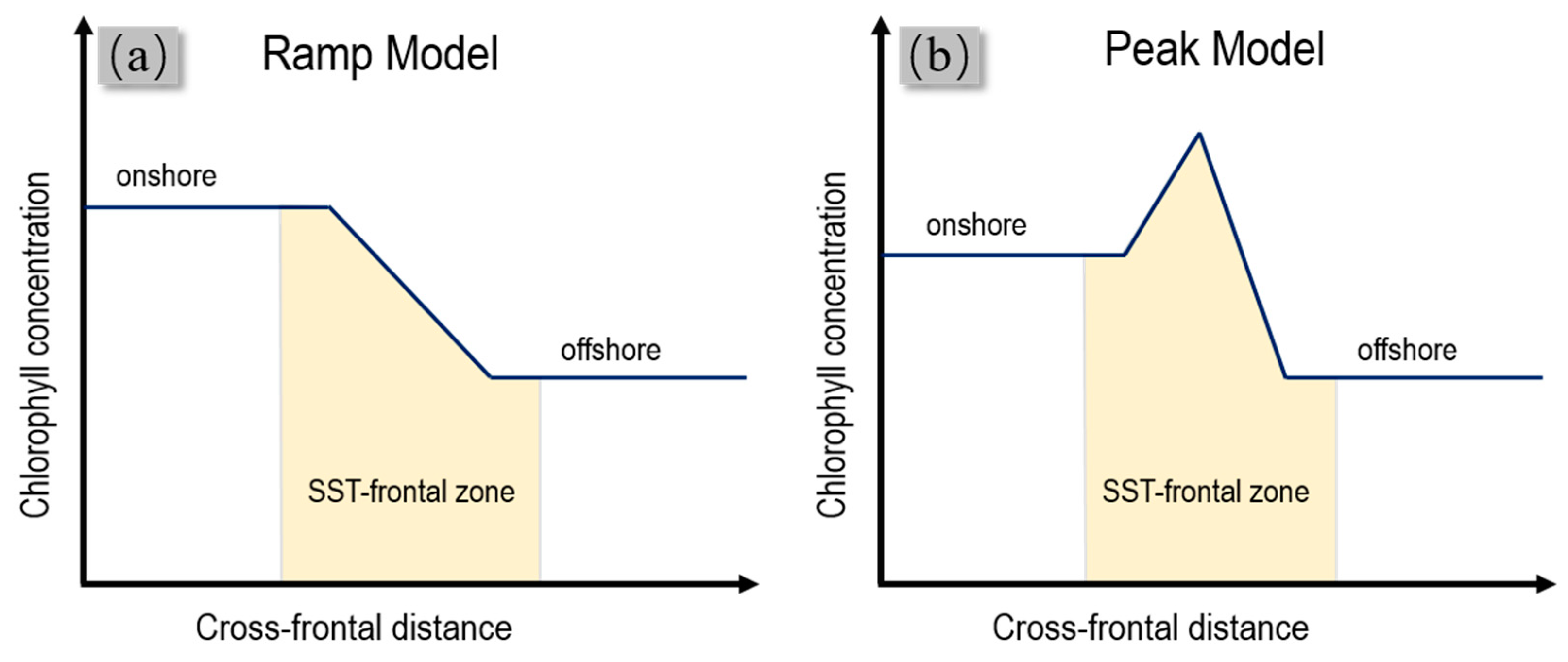
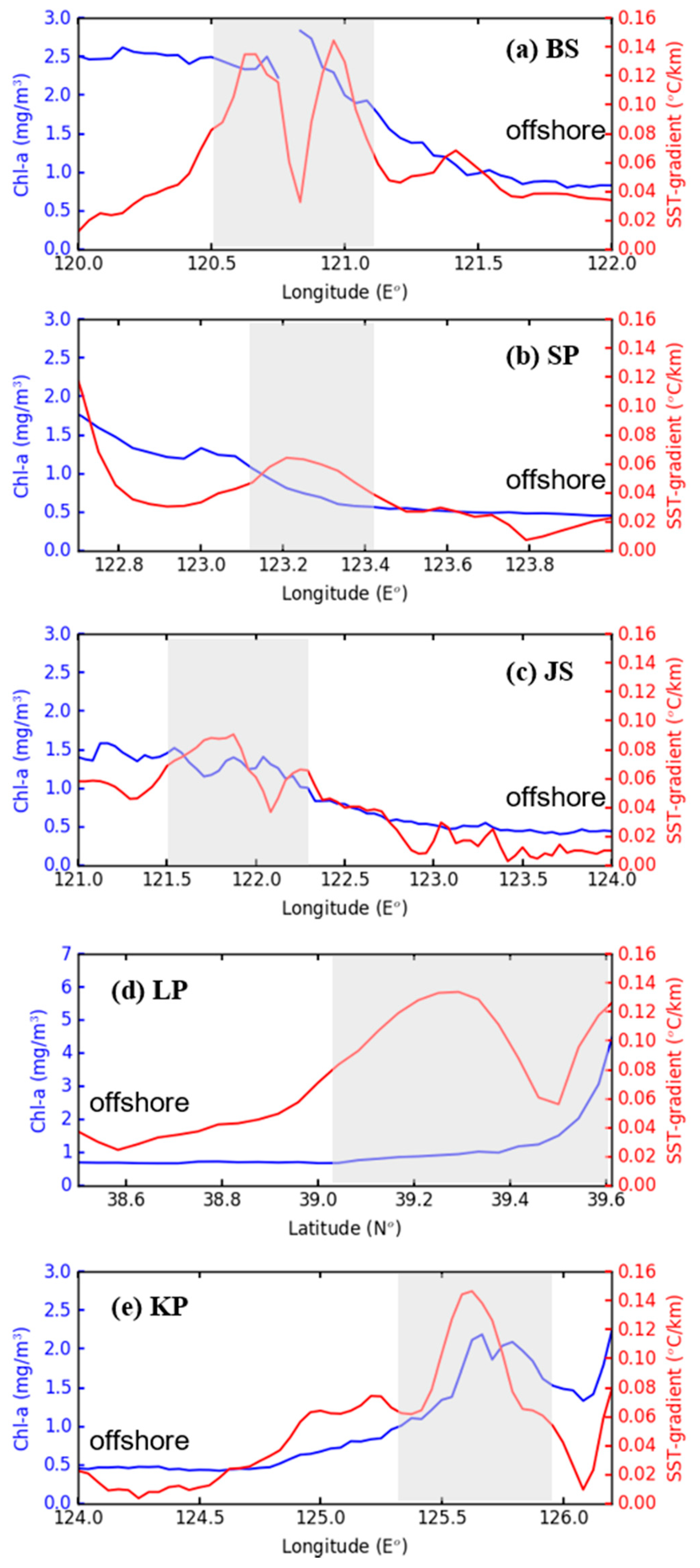
4.2. Relationship between Chl-a Fronts and SST Fronts

As shown in Figure 4 and Figure 7, although SST fronts were strong in winter, the deep vertical mixing and light-limitation inhibited the formation of chl-a fronts [32,40,43], as discussed in Section 4.1. Therefore, there was no distinct links between the chl-a front and SST front in winter. In summer, the location of Chl-a fronts was in good correspondence to that of the SST fronts. Meanwhile, the intensity of the chl-a fronts was also consistent with that of the SST front in summer. For instance, strong LP and KP chl-a fronts corresponded to strong LP and KP SST fronts; SP and JS chl-a fronts with weak SST fronts were weaker than other chl-a fronts (Figure 6 and Figure 8).
Chl-a fronts always coincided with SST fronts [2]. Basically, there are two main patterns of chl-a across the SST-frontal zone (Figure 10), which were summarized by [2]. SST fronts along the coast could act like dynamic barriers to momentum and offshore water transport [2,44], and thus become boundaries between higher coastal biomass on one side, and lower offshore biomass on the other (i.e., ‘Ramp Model’ in Figure 10a). SST fronts could also induce maximum chl-a concentrations along the front (i.e., ‘Peak Model’ in Figure 10b) via convergence and nutrient upwelling, and, in both cases, the strongest chl-a gradients (i.e., chl-a fronts) are located at the SST frontal zone.
In order to investigate which model best described the summer Yellow Sea fronts, the chl-a along five transects cross different fronts in August were summarized in Figure 11. The chl-a of four transects (i.e., BS, SP, JS, and LP) increased from offshore to coast and rapidly increased in the SST front region. Based on the chl-a pattern, the four transects were determined to belong to the Ramp model (Figure 11a–d), which indicates that the SST fronts separated the high coastal chl-a from the low offshore chl-a by limiting coastal-offshore water exchange. The chl-a along the KP transect increased at the SST-front region (125.5° E–126° E), then decreased onshore, but maintained a relatively higher concentration near the coast (Figure 11e). This pattern is consistent with the Peak Model, which might be related to the strong KP tidal front. Overall, our results suggest that the SST frontal region in the YB sea should be considered a transition zone (i.e., Ramp Model) in most cases, which separates well-mixed from stratified waters and limits the exchange of nutrient- and chl-a-containing water. The Ramp Model appeared to better describe the shallow coastal waters where water is eutrophic due to abundant terrestrial nutrients, such as in the coastal zone of the northwest Atlantic [14] and off the west coast of Denmark [45].
Moreover, there was a time lag of approximately two months between the chl-a front maximum occurrence (i.e., approximately in August) compared to that of SST fronts (i.e., approximately in June). The maximum occurrence of chl-a fronts was largely consistent with the maximum offshore stratification and rainfall, which were strongest from late July to early August [46,47]. The stratification and rainfall could influence the offshore and coastal chl-a by changing the nutrient concertation. This suggests that the runoff and stratification could be helpful for the enhancement of chl-a fronts, while the presence of SST front is a pre-requisite for the formation of a chl-a front in summer. The nutrient and chl-a boundaries established by SST fronts facilitated the formation and preservation of said chl-a fronts.

4.3. Implication from the Chl-a Front

Both our results (Figure 7), as well as a previous study [6], suggest that the strong winter SST fronts in the Yellow Sea tend to fade and even disappear in other seasons, especially in the SP front. In summer, strong surface heating could induce the relatively uniform SST and greatly weaken the SST fronts. However, the satellite results clearly demonstrated the formation of chl-a fronts in the YB Sea in summer. In situ observed and model results from Lü et al. (2010) indicated that a strong temperature front at the bottom layer existed under the strong SP chl-a front offshore the Shandong Peninsula in summer but the SST front is weak [38]. The front at the bottom layer resulted from the convergence of well-mixed and stratified waters. Due to phytoplankton photosynthesis, chl-a mainly concentrated on the sea surface. The relative chl-a concentration could reflect the vertical water structure (i.e., well-mixed or stratified) under the sea surface in shelf seas. Due to limited nutrient supply in the upper layer due to stratification, chl-a in stratified waters was relatively low, while chl-a was usually relatively high in well-mixed and eutrophic coastal waters. Therefore, surface chl-a fronts were found to be good indicators to diagnose the location of internal physical fronts or vertical structure boundaries.
Furthermore, both the variable chl-a and SST fronts consistently occurred within steep seabed slopes (ratio of slope > 1%) (Figure 12). Several studies have indicated that topography is a potentially important factor for the formation of fronts (e.g., [17,39]). Topography likely influences the formation of fronts through two main mechanisms. First, based on the geostrophic balance or conservation of potential vorticity, the flow should follow the isobaths [1]. Therefore, little heat and material transport occur across steep slopes, which led to different nutrient environments between coastal and offshore waters, thus facilitating front formation. Second, tidal fronts usually form in locations with steep slopes [17,38]. Since the formation of tidal fronts is related to the energy balance of heating and tidal mixing, which is proportional to the water depth [48], the depth of steep-sloped regions with variable water depths was easier to determine when said energy balance was known. These tidal fronts could be regarded as the boundary between well-mixed and stratified waters, which influenced chl-a concentration and limited its cross-frontal exchange, as discussed in Section 4.1 and Section 4.2. Both the limitation of cross-isobath exchange and the tidal front facilitated the formation of chl-a fronts in location with steep slopes, suggesting that seabed slope may be a valid indicator of the location of oceanic fronts on the climatological scale.

5. Conclusions

Based on the monthly mean chl-a concentration retrieved from MODIS satellite data, the seasonal variations of sea surface chl-a fronts in the YB Sea were characterized. In the YB Sea, five distinct chl-a fronts (i.e., the Bohai strait front, Shandong Peninsula front, Jiangsu front, Liaodong Peninsula front, and Korean Peninsula front) occurred roughly along the 40 m isobaths in summer and faded in other seasons. The location of chl-a fronts was consistent with that of SST fronts, both of which coincided with the location of a steep slope (ratio of slope > 1%). It would seem more appropriate to consider SST fronts in the YB Sea as transition zones in most cases, which separate high coastal chl-a from low offshore chl-a concentrations. Strong chl-a fronts in summer were likely induced by the chl-a bloom in eutrophic coastal waters and surface chl-a fading in the strongly stratified offshore waters together with the coastal physical fronts. Although the SST fronts were strong in winter, the light limitation resulting from high suspended sediment concentrations in coastal waters and the deep mixed layer from strong vertical mixing in offshore waters were the likely cause of low chl-a in both coastal and offshore waters, which presumably suppressed the formation of chl-a fronts. The seasonal and spatial pattern of the fronts would be helpful for understanding the temporal-spatial variability of the hydrodynamics and ecosystem and providing a scientific reference for marine fisheries and planning. Due to the limitation of the data, this study only focused on the seasonal variability of the fronts. The interannual variability of the fronts still needs to be further investigated using data with better space-time continuity.

Author Contributions

Conceptualization, L.X. and L.L.; methodology, Y.W. and L.L.; writing—original draft preparation, L.X., H.L. and L.L. All authors have read and agreed to the published version of the manuscript.

Funding

The study was financially supported by the Open Research Fund of State Key Laboratory of Estuarine and Coastal Research (Grant number SKLEC-KF202105).

Institutional Review Board Statement

Not applicable.

Informed Consent Statement

Not applicable.

Data Availability Statement

These satellite data used in this study can be downloaded from the U.S. National Aeronautics and Space Administration (NASA) website (http://oceancolor.gsfc.nasa.gov, accessed on 15 June 2020).

Acknowledgments

The authors thank the National Oceanic and Atmospheric Administration and the European Space Agency for their support regarding the satellite data.

Conflicts of Interest

The authors declare no conflict of interest.

References

  1. Cushman-Roisin, B.; Beckers, J.M. Introduction to Geophysical Fluid Dynamics: Physical and Numerical Aspects; Academic Press: Cambridge, MA, USA, 2011. [Google Scholar]
  2. Belkin, I.M.; O’Reilly, J.E. An algorithm for oceanic front detection in chlorophyll and SST satellite imagery. J. Marine. Syst. 2009, 78, 319–326. [Google Scholar] [CrossRef]
  3. Acha, E.M.; Piola, A.; Iribarne, O.; Mianzan, H. Ecological Processes at Marine Fronts; Springerbriefs in Environmental Science: Basingstoke, UK, 2015. [Google Scholar]
  4. Muñoz, M.; Reul, A.; García-Martínez, M.; Plaza, F.; Bautista, B.; Moya, F.; Vargas-Yáñez, M. Oceanographic and Bathymetric Features as the Target for Pelagic MPA Design: A Case Study on the Cape of Gata. Water 2018, 20, 1043. [Google Scholar] [CrossRef] [Green Version]
  5. Zhang, Y.; Li, D.; Wang, K.; Xue, B. Contribution of Biological Effects to the Carbon Sources/Sinks and the Trophic Status of the Ecosystem in the Changjiang (Yangtze) River Estuary Plume in Summer as Indicated by Net Ecosystem Production Variations. Water 2019, 6, 1264. [Google Scholar] [CrossRef] [Green Version]
  6. Hickox, R.; Belkin, I.; Cornillon, P.; Shan, Z. Climatology and seasonal variability of ocean fronts in the East China, Yellow and Bohai seas from satellite SST data. Geophys. Res. Lett. 2000, 27, 2945–2948. [Google Scholar] [CrossRef] [Green Version]
  7. Vazquez-Cuervo, J.; Dewitte, B.; Chin, T.M.; Armstrong, E.M.; Purca, S.; Alburqueque, E. An analysis of SST gradients off the Peruvian Coast: The impact of going to higher resolution. Remote. Sens. Environ. 2013, 131, 76–84. [Google Scholar] [CrossRef]
  8. O’Reilly, J.E.; Maritorena, S.; Mitchell, B.G.; Seigal, D.; Carder, K.; Garver, S.; Kahru, M.; McClain, C. Ocean color chlorophyll algorithms for SeaWiFS. J. Geophys. Res. 1998, 103, 24937–24954. [Google Scholar] [CrossRef] [Green Version]
  9. Mercado, J.; León, P.; Salles, S.; Cortés, D.; Yebra, L.; Gómez-Jakobsen, F.; Herrera, I.; Alonso, A.; Sánchez, A.; Valcárcel-Pérez, N.; et al. Time Variability Patterns of Eutrophication Indicators in the Bay of Algeciras (South Spain). Water 2018, 7, 938. [Google Scholar] [CrossRef] [Green Version]
  10. Shi, L.; Mao, Z.; Wu, J.; Liu, M.; Zhang, Y.; Wang, Z. Variations in spectral absorption properties of phytoplankton, non-algal particles and chromophoric dissolved organic matter in Lake Qiandaohu. Water 2017, 5, 352. [Google Scholar] [CrossRef] [Green Version]
  11. Polovina, J.J.; Howell, E.; Kobayashi, D.R.; Seki, M.P. The Transition Zone Chlorophyll Front, a dynamic global feature defining migration and forage habitat for marine resources. Prog. Oceanogr. 2001, 49, 469–483. [Google Scholar] [CrossRef]
  12. Legeckis, R.; Brown, C.W.; Chang, P.S. Geostationary satellites reveal motions of ocean surface fronts. J. Mar. Syst. 2002, 37, 3–15. [Google Scholar] [CrossRef]
  13. Hu, J.Y.; Kawamura, H.; Tang, D.L. Tidal front around the Hainan Island, northwest of the South China Sea. J. Geophys. Res. Oceans 2003, 108, 3342. [Google Scholar] [CrossRef]
  14. Stegmann, P.M.; Ullman, D.S. Variability in chlorophyll and sea surface temperature fronts in the Long Island Sound outflow region from satellite observations. J. Geophys. Res. Oceans 2004, 109, C3S–C7S. [Google Scholar] [CrossRef] [Green Version]
  15. Liu, Z.; Wang, H.; Guo, X.; Qiang, W.; Gao, H. The age of Yellow River water in the Bohai Sea. J. Geophys. Res. Oceans 2012, 117, 317–323. [Google Scholar] [CrossRef] [Green Version]
  16. Guo, W.; Wu, G.; Liang, B.; Xu, T.; Chen, X.; Yang, Z.; Xie, M.; Jiang, M. The influence of surface wave on water exchange in the Bohai Sea. Cont. Shelf Res. 2016, 118, 128–142. [Google Scholar] [CrossRef]
  17. Huang, D.; Tao, Z.; Feng, Z. Sea-surface temperature fronts in the Yellow and East China Seas from TRMM microwave imager data. Deep Sea Res. Part II Top. Stud. Oceanogr. 2010, 57, 1024. [Google Scholar] [CrossRef]
  18. Su, J. A review of circulation dynamics of the China coastal seas. Acta Oceanol. Sin. 2001, 4, 1–16. [Google Scholar]
  19. Zhang, S.W.; Wang, Q.Y.; Lü, Y.; Cui, H.; Yuan, Y.L. Observation of the seasonal evolution of the Yellow Sea Cold Water Mass in 1996–1998. Cont. Shelf Res. 2008, 28, 457. [Google Scholar] [CrossRef]
  20. Xia, C.; Qiao, F.; Yang, Y.; Ma, J.; Yuan, Y. Three-dimensional structure of the summertime circulation in the Yellow Sea from a wave-tide-circulation coupled model. J. Geophys. Res. Oceans 2006, 111, 1–19. [Google Scholar] [CrossRef]
  21. Jiang, W.; Thomas, P.; Jun, S.; Andreas, S. SPM transport in the Bohai Sea: Field experiments and numerical modelling. J. Mar. Syst. 2004, 44, 175–188. [Google Scholar] [CrossRef]
  22. Liu, S.M.; Zhang, J.; Chen, S.Z.; Chen, H.T.; Hong, G.H.; Wei, H.; Wu, Q.M. Inventory of nutrient compounds in the Yellow Sea. Cont. Shelf Res. 2003, 23, 1161–1174. [Google Scholar] [CrossRef]
  23. Liu, S.M.; Li, L.W.; Zhang, Z. Inventory of nutrients in the Bohai. Cont. Shelf Res. 2011, 31, 1797. [Google Scholar]
  24. Son, S.H.; Kim, Y.H.; Kwon, J.; Kim, H.; Park, K. Characterization of spatial and temporal variation of suspended sediments in the Yellow and East China Seas using satellite ocean color data. Mapping GlSci. Remote Sens. 2014, 51, 212–226. [Google Scholar] [CrossRef]
  25. Bian, C.; Jiang, W.; Quan, Q.; Wang, T.; Greatbatch, R.J.; Li, W. Distributions of suspended sediment concentration in the Yellow Sea and the East China Sea based on field surveys during the four seasons of 2011. J. Mar. Syst. 2013, 121–122, 24–35. [Google Scholar] [CrossRef]
  26. Liu, F.; Su, J.; Moll, A.; Krasemann, H.; Chen, X.; Pohlmann, T.; Wirtz, K. Assessment of the summer-autumn bloom in the Bohai Sea using satellite images to identify the roles of wind mixing and light conditions. J. Mar. Syst. 2014, 129, 303–317. [Google Scholar] [CrossRef] [Green Version]
  27. Fan, W.; Chuanyu, L.; Qingjia, M. Effect of the Yellow Sea warm current fronts on the westward shift of the Yellow Sea warm tongue in winter. Cont. Shelf Res. 2012, 45, 98–107. [Google Scholar]
  28. Lin, L.; Liu, D.; Luo, C.; Xie, L. Double fronts in the Yellow Sea in summertime identified using sea surface temperature data of multi-scale ultra-high resolution analysis. Cont. Shelf Res. 2019, 175, 76–86. [Google Scholar] [CrossRef]
  29. Lee, M.; Chang, Y.; Shimada, T. Seasonal evolution of fine-scale sea surface temperature fronts in the East China Sea. Deep Sea Res. Part II Top. Stud. Oceanogr. 2015, 119, 20–29. [Google Scholar] [CrossRef]
  30. Wang, Y.; Liu, D.; Tang, D.L. Application of a generalized additive model (GAM) for estimating chlorophyll-a concentration from MODIS data in the Bohai and Yellow Seas. China. Int. J. Remote Sens. 2017, 3, 639–661. [Google Scholar] [CrossRef]
  31. Karimova, S. Hydrological fronts seen in visible and infrared MODIS imagery of the Black Sea. Int. J. Remote Sens. 2014, 16, 6113–6134. [Google Scholar] [CrossRef]
  32. Lin, L.; Wang, Y.; Liu, D. Vertical average irradiance shapes the spatial pattern of winter chlorophyll-a in the Yellow Sea. Estuar. Coast. Shelf Sci. 2019, 224, 11–19. [Google Scholar] [CrossRef]
  33. Zeng, X.; Belkin, I.M.; Peng, S.; Li, Y. East Hainan upwelling fronts detected by remote sensing and modelled in summer. Int. J. Remote Sens. 2014, 11–12, 4441–4451. [Google Scholar] [CrossRef]
  34. Fu, M.; Zongling, W.; Yan, L.; Ruixiang, L.; Ping, S.; Xiuhua, W.; Xuezheng, L.; Jingsong, G. Phytoplankton biomass size structure and its regulation in the Southern Yellow Sea (China): Seasonal variability. Cont. Shelf Res. 2009, 29, 2194. [Google Scholar] [CrossRef]
  35. Shi, J.; Liu, Y.; Mao, X.; Guo, X.; Wei, H.; Gao, H. Interannual variation of spring phytoplankton bloom and response to turbulent energy generated by atmospheric forcing in the central Southern Yellow Sea of China: Satellite observations and numerical model study. Cont. Shelf Res. 2016, S176438184. [Google Scholar] [CrossRef]
  36. Liu, D.; Wang, Y. Trends of satellite derived chlorophyll-a (1997–2011) in the Bohai and Yellow Seas, China: Effects of bathymetry on seasonal and inter-annual patterns. Prog. Oceanogr. 2013, 116, 154–166. [Google Scholar] [CrossRef]
  37. Xu, Y.; Ishizaka, J.; Yamaguchi, H.; Siswanto, E.; Wang, S. Relationships of interannual variability in SST and phytoplankton blooms with giant jellyfish (Nemopilema nomurai) outbreaks in the Yellow Sea and East China Sea. J. Oceanogr. 2013, 69, 511–526. [Google Scholar] [CrossRef] [Green Version]
  38. Lü, X.; Fangli, Q.; Changshui, X.; Guansuo, W.; Yeli, Y. Upwelling and surface cold patches in the Yellow Sea in summer: Effects of tidal mixing on the vertical circulation. Cont. Shelf Res. 2010, 30, 632. [Google Scholar] [CrossRef]
  39. Chen, C.T.A. Chemical and physical fronts in the Bohai, Yellow and East China seas. J. Mar. Syst. 2009, 78, 394–410. [Google Scholar] [CrossRef]
  40. Huang, D.; Fan, X.; Xu, D.; Tong, Y.; Su, J. Westward shift of the Yellow Sea warm salty tongue. Geophys. Res. Lett. 2005, 32, 348–362. [Google Scholar] [CrossRef]
  41. Shang, S.; Lee, Z.; Wei, G. Characterization of MODIS-derived euphotic zone depth: Results for the China Sea. Remote Sens. Environ. 2011, 115, 180–186. [Google Scholar] [CrossRef]
  42. Zhou, F.; Xuan, J.; Huang, D.; Liu, C.; Sun, J. The timing and the magnitude of spring phytoplankton blooms and their relationship with physical forcing in the central Yellow Sea in 2009. Deep Sea Res. Part II Top. Stud. Oceanogr. 2013, 97, 4–15. [Google Scholar] [CrossRef]
  43. Wei, Q.S.; Yu, Z.G.; Wang, B.D.; Fu, M.Z.; Xia, C.S.; Liu, L.; Zhan, R. Coupling of the spatial–temporal distributions of nutrients and physical conditions in the southern Yellow Sea. J. Mar. Syst. 2016, 156, 30–45. [Google Scholar] [CrossRef]
  44. Chen, C.; Jianrong, Z.; KiRyong, K.; Hedong, L.; Elise, R.; Sarah, A.G.; Judith, W.B. Cross-frontal transport along the Keweenaw coast in Lake Superior: A Lagrangian model study. Dyn. Atmos. Oceans 2002, 36, 102. [Google Scholar] [CrossRef]
  45. Munk, P. Differential growth of larval sprat Sprattus sprattus across a tidal front in the eastern North sea. Mar. Ecol. Prog. Ser. 1993, 1–2, 17–27. [Google Scholar] [CrossRef]
  46. Chu, P.C.; Fralick, C.R.; Haeger, S.D.; Carron, M.J. A parametric model for the Yellow Sea thermal variability. J. Geophys. Res. Oceans 1997, 102, 10499. [Google Scholar] [CrossRef] [Green Version]
  47. Qian, W.; Kang, H.-S.; Lee, D.-K. Distribution of seasonal rainfall in the East Asian monsoon region. Theor. Appl. Climatol. 2002, 73, 151–168. [Google Scholar] [CrossRef]
  48. Simpson, J.H.; Hunter, J.R. Fronts in the Irish Sea. Nature 1974, 250, 404–406. [Google Scholar] [CrossRef]
Figure 1. (a) Location and bathymetry of the Yellow and Bohai Seas. (b) Winter circulation pattern diagram, where red arrows and blue arrows represent the Yellow sea warm current and cold coastal currents, respectively. (c) Summer circulation (gray arrows) diagram, where the blue area represents the Yellow Sea cool water mass.
Jmse 09 01301 g001
Figure 2. Monthly averaged chl-a concentration (mg/m3). The gray lines denote the 40 m isobath.
Jmse 09 01301 g002
Figure 3. Average monthly chl-a concentration in the Bohai Sea, the Yellow Sea Coast, and the Yellow Sea offshore zones.
Jmse 09 01301 g003
Figure 4. Seasonal chl-a front magnitudes (expressed as ratios). Five chl-a fronts in summer: 1, Bohai strait (BS) front; 2, Shandong Peninsula (SP) front; 3, Jiangsu (JS) front; 4, Liaodong Peninsula (LP) front; 5, Korean Peninsula (KP) front. The gray lines denote the 40 m isobath.
Jmse 09 01301 g004
Figure 5. The standard deviation of the chl-a front in summer from 2002 to 2016.
Jmse 09 01301 g005
Figure 6. Monthly magnitude of the five chl-a fronts depicted in Figure 4.
Jmse 09 01301 g006
Figure 7. Seasonal SST front magnitudes (°C/km). The yellow lines represent the five summer chl-a front outlines. The gray lines denote the 40 m isobath.
Jmse 09 01301 g007
Figure 8. Monthly SST front magnitudes averaged over the five chl-a front zones (gray lines in Figure 7).
Jmse 09 01301 g008
Figure 9. Average monthly rainfall in the area around the Yellow and Bohai Seas.
Jmse 09 01301 g009
Figure 10. Two kinds of models of chl-a distribution across the SST-frontal zone, redrawn after [2]. (a) Ramp Model. (b) Peak Model.
Jmse 09 01301 g010
Figure 11. Chl-a concentration and SST gradient across the five fronts in August. (ae) Transects along 38.3° N, 37° N, 34° N, 123.8° E, and 37° N, respectively. The gray shadings indicate the SST-frontal zones.
Jmse 09 01301 g011
Figure 12. Map of the sea bottom slope (ratio of slope, %). Dashed lines show the location of five chl-a fronts.
Jmse 09 01301 g012
Publisher’s Note: MDPI stays neutral with regard to jurisdictional claims in published maps and institutional affiliations.

