
A Stereo Matching Method for 3D Image Measurement of Long-Distance Sea Surface


Abstract
:
1. Introduction
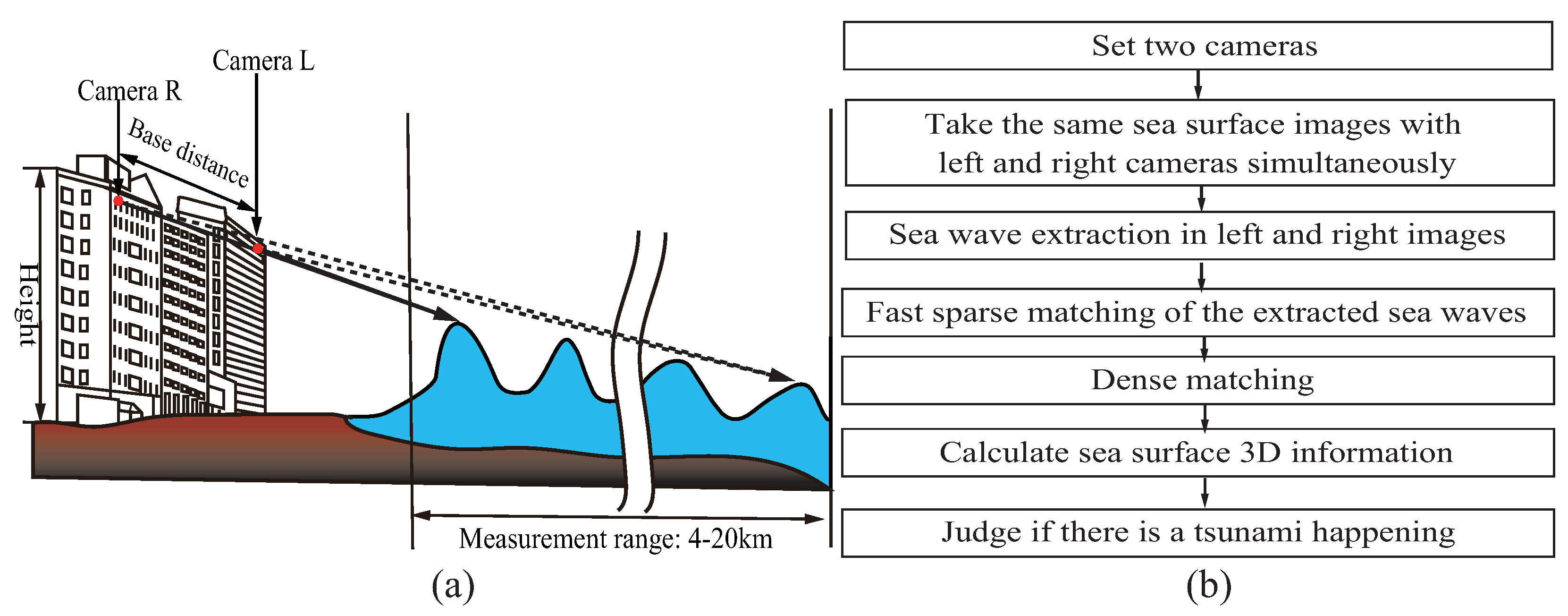
2. Method
2.1. Motivations
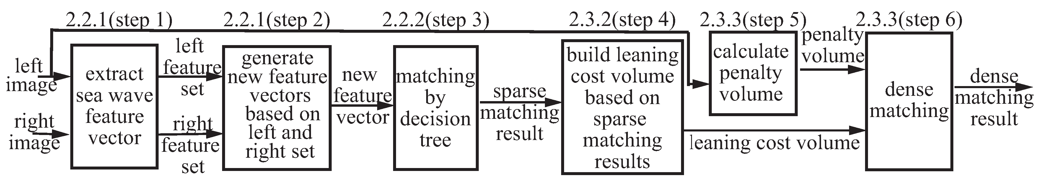
2.2. Sparse Matching by Feature Vector
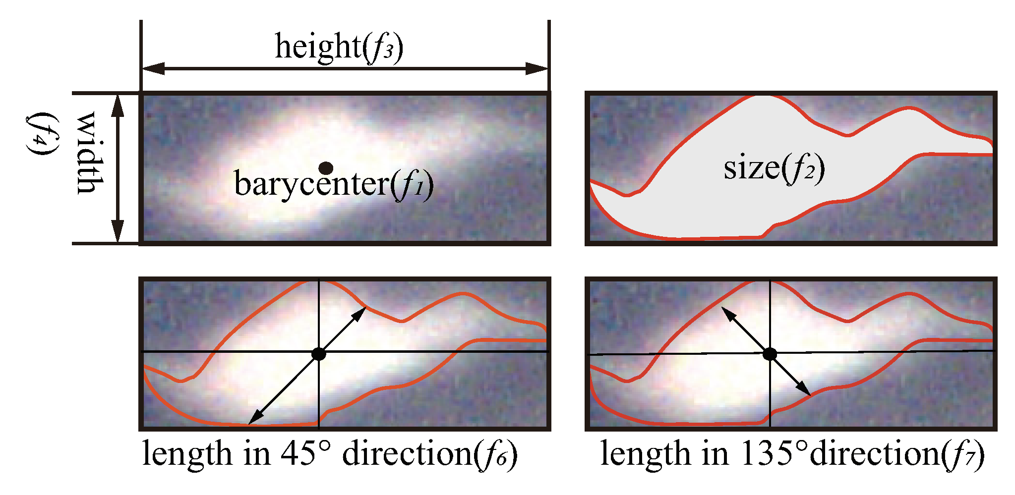
2.2.1. Feature Vector Definition
2.2.2. Fast Matching by Decision Tree
2.3. Dense Matching by Building Leaning Cost Volume
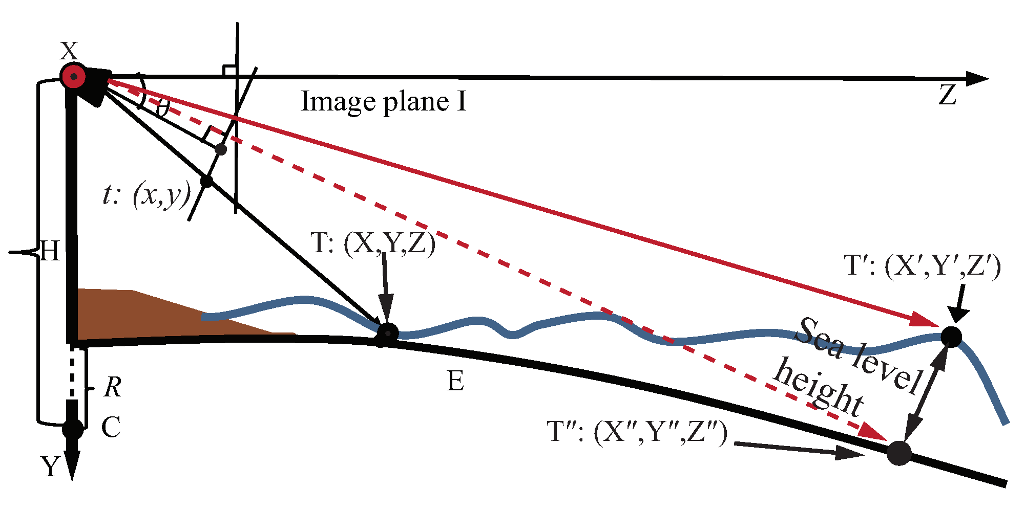
2.3.1. Relationship between Disparity and y Coordinates of Sea Surface Images
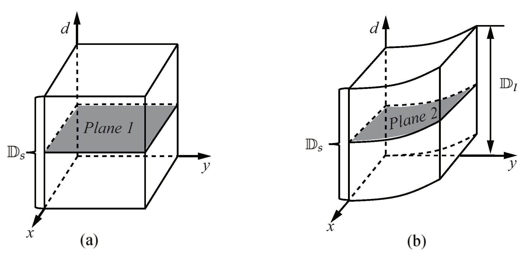
2.3.2. Build Leaning Cost Volume
2.3.3. Fast Dense Matching
3. Experiment Results
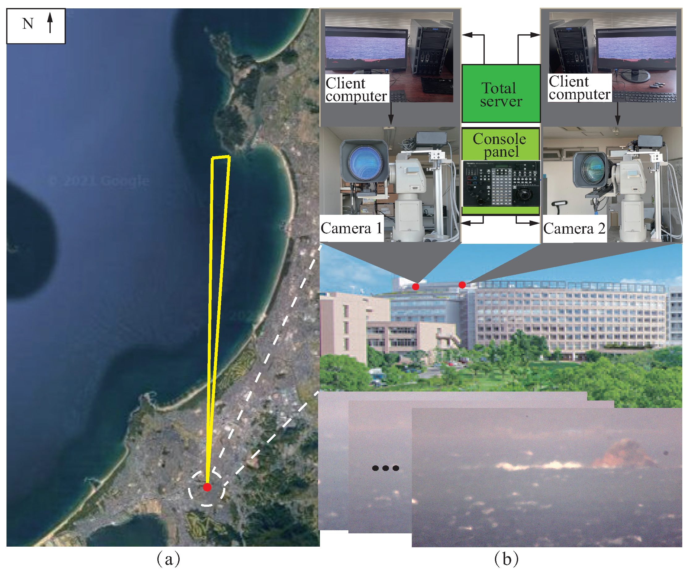
3.1. Configuration of the Proposed System
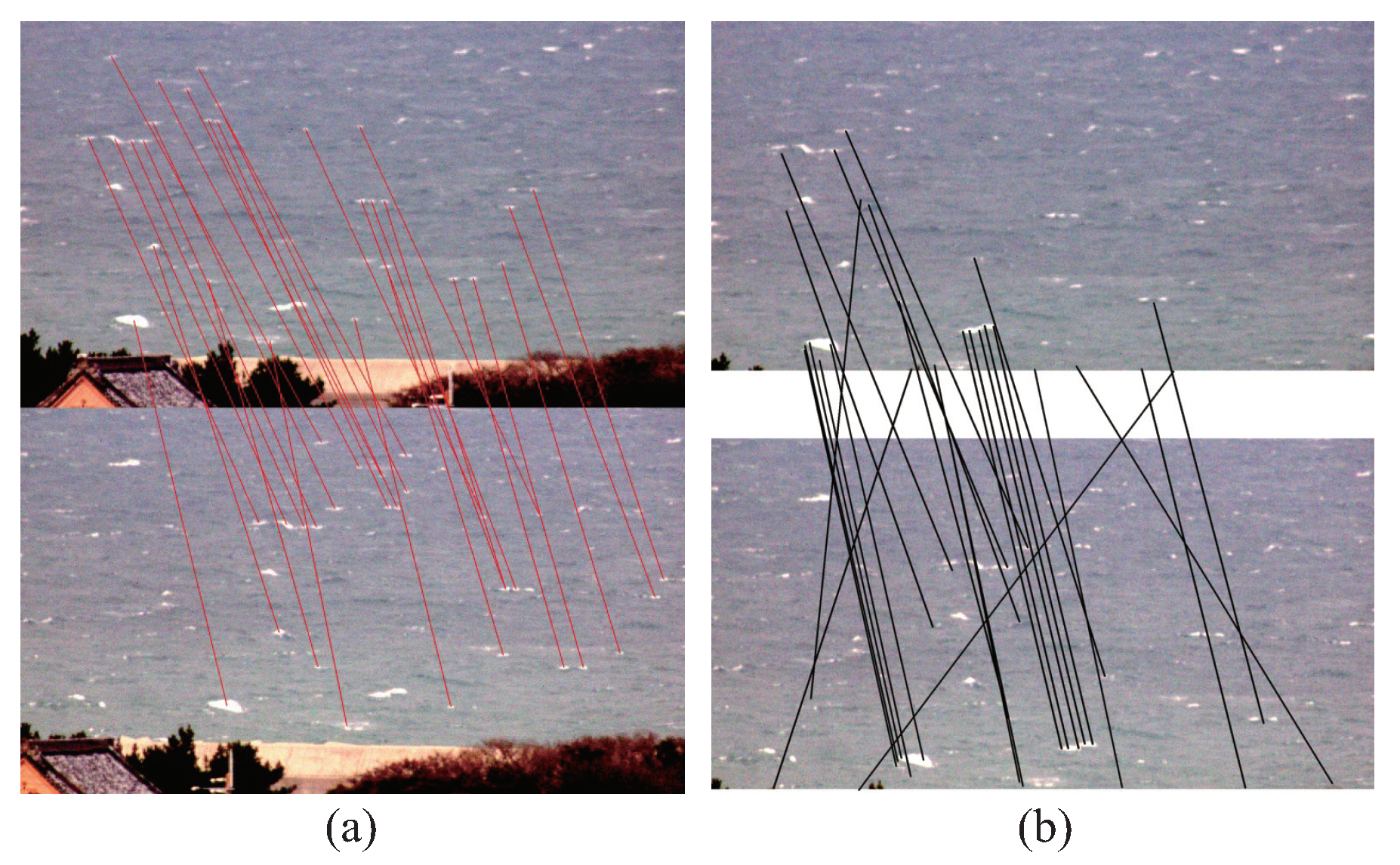
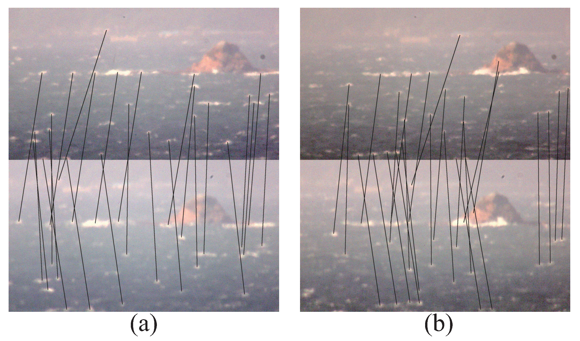
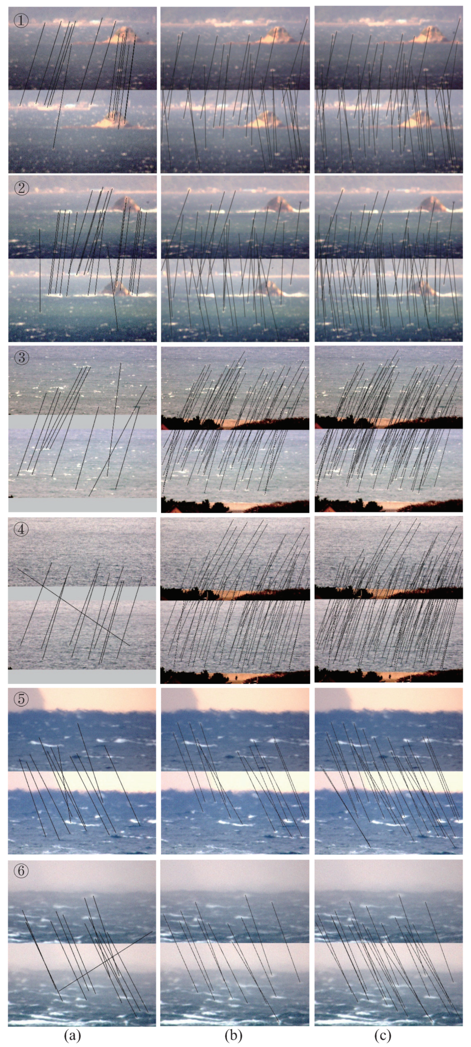
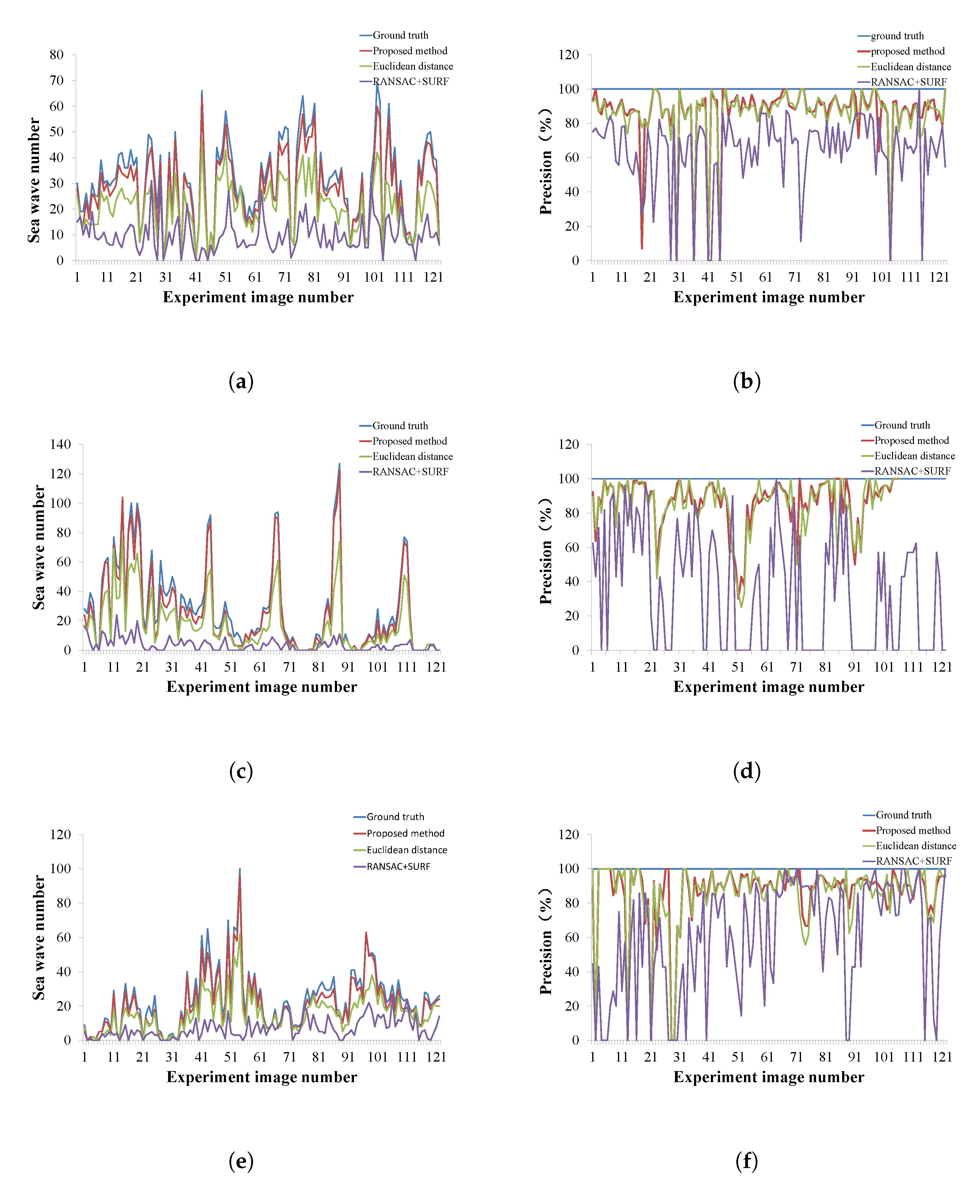
3.2. Sparse Matching Results
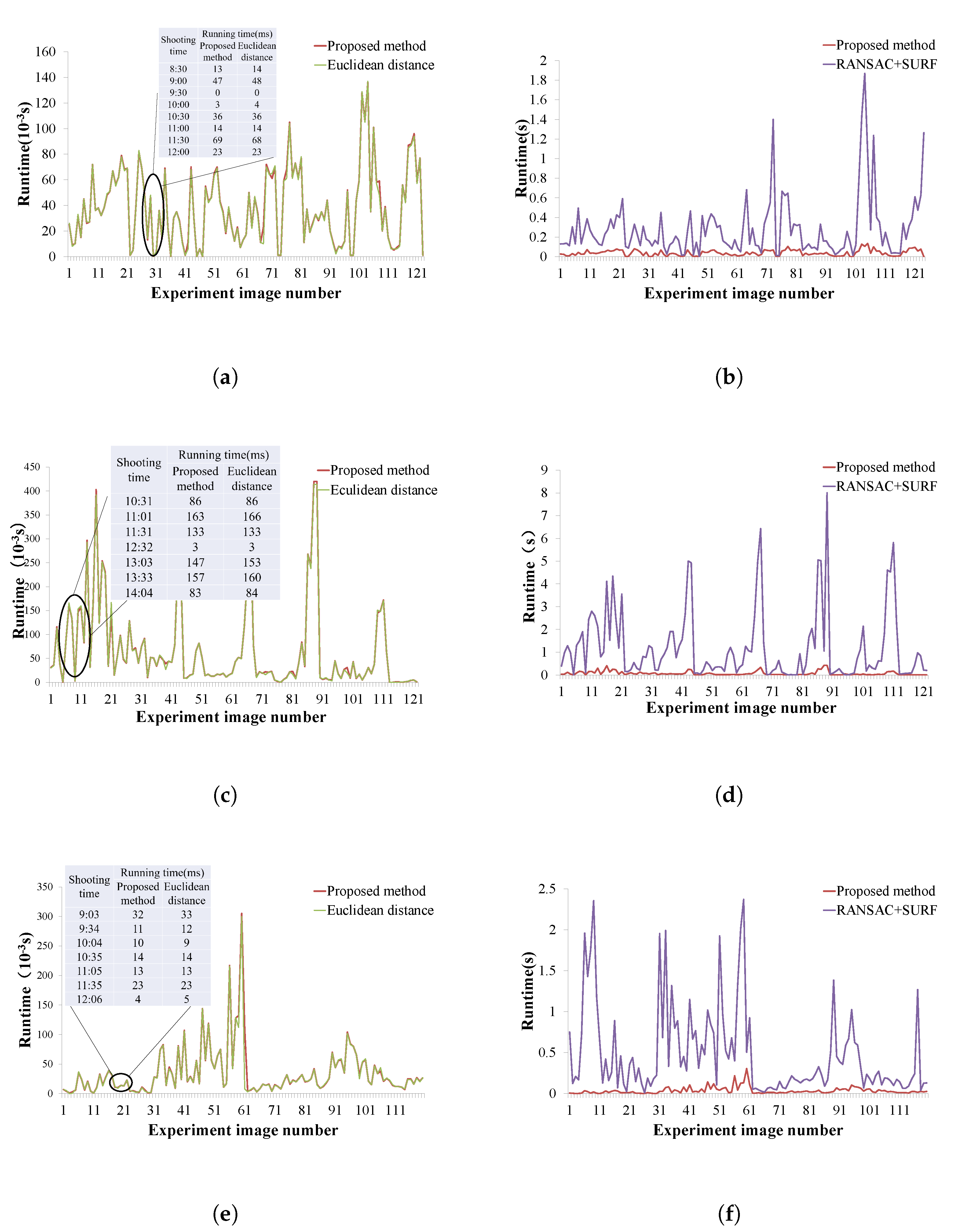
3.3. Computational Complexity
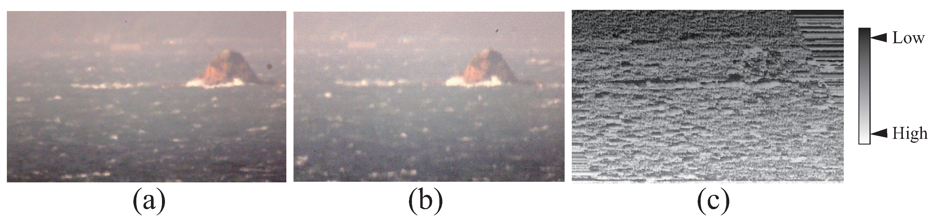
3.4. Dense Matching Results
4. Discussion and Conclusions
Author Contributions
Funding
Institutional Review Board Statement
Informed Consent Statement
Acknowledgments
Conflicts of Interest
References
- Hirshorn, B.; Weinstein, S.; Tsuboi, S. On the application of Mwp in the near field and the March 11, 2011 Tohoku earthquake. Pure Appl. Geophys. 2013, 170, 975–991. [Google Scholar] [CrossRef]
- Meinig, C.; Stalin, S.E.; Nakamura, A.I.; González, F.; Milburn, H.B. Technology developments in real-time tsunami measuring, monitoring and forecasting. In Proceedings of the OCEANS 2005 MTS/IEEE, Washington, DC, USA, 17–23 September 2005; pp. 1673–1679. [Google Scholar]
- NRI for Earth Science; Resilience, D. Seafloor Observation Network for Earthquakes and Tsunamis along the Japan Trench. Available online: http://www.bosai.go.jp/inline/seibi/seibi01.html/ (accessed on 2 March 2021).
- Tatehata, H. The new tsunami warning system of the Japan Meteorological Agency. In Perspectives on Tsunami Hazard Reduction; Springer: Berlin/Heidelberg, Germany, 1997; pp. 175–188. [Google Scholar]
- Mori, N.; Takahashi, T.; The 2011 Tohoku Earthquake Tsunami Joint Survey Group. Nationwide Post Event Survey and Analysis of the 2011 Tohoku Earthquake Tsunami. Coast. Eng. J. 2012, 54, 1250001-1–1250001-27. [Google Scholar] [CrossRef] [Green Version]
- Lauterjung, J.; Letz, H. 10 Years Indonesian Tsunami Early Warning System: Experiences, Lessons Learned and Outlook; GFZ German Research Centre for Geosciences: Potsdam, Germany, 2017. [Google Scholar]
- Nayak, S.; Kumar, T.S. Indian tsunami warning system. Int. Arch. Photogramm. Remote Sens. Spat. Inf. Sci. Beijing 2008, 37, 1501–1506. [Google Scholar]
- Allen, S.; Greenslade, D. Developing tsunami warnings from numerical model output. Nat. Hazards 2008, 46, 35–52. [Google Scholar] [CrossRef]
- Larson, K.M.; Lay, T.; Yamazaki, Y.; Cheung, K.F.; Ye, L.; Williams, S.D.; Davis, J.L. Dynamic sea level variation from GNSS: 2020 Shumagin earthquake tsunami resonance and Hurricane Laura. Geophys. Res. Lett. 2021, 48, e2020GL091378. [Google Scholar] [CrossRef]
- Yu, K. Tsunami-wave parameter estimation using GNSS-based sea surface height measurement. IEEE Trans. Geosci. Remote Sens. 2014, 53, 2603–2611. [Google Scholar] [CrossRef]
- Mulia, I.E.; Hirobe, T.; Inazu, D.; Endoh, T.; Niwa, Y.; Gusman, A.R.; Tatehata, H.; Waseda, T.; Hibiya, T. Advanced tsunami detection and forecasting by radar on unconventional airborne observing platforms. Sci. Rep. 2020, 10, 1–10. [Google Scholar]
- Shemdin, O.H.; Tran, H.M.; Wu, S. Directional measurement of short ocean waves with stereophotography. J. Geophys. Res. Ocean. 1988, 93, 13891–13901. [Google Scholar] [CrossRef]
- Wanek, J.M.; Wu, C.H. Automated trinocular stereo imaging system for three-dimensional surface wave measurements. Ocean. Eng. 2006, 33, 723–747. [Google Scholar] [CrossRef]
- Bechle, A.J.; Wu, C.H. Virtual wave gauges based upon stereo imaging for measuring surface wave characteristics. Coast. Eng. 2011, 58, 305–316. [Google Scholar] [CrossRef]
- Kosnik, M.V.; Dulov, V.A. Extraction of short wind wave spectra from stereo images of the sea surface. Meas. Sci. Technol. 2010, 22, 015504. [Google Scholar] [CrossRef]
- Benetazzo, A. Measurements of short water waves using stereo matched image sequences. Coast. Eng. 2006, 53, 1013–1032. [Google Scholar] [CrossRef]
- Gallego, G.; Yezzi, A.; Fedele, F.; Benetazzo, A. A variational stereo method for the three-dimensional reconstruction of ocean waves. IEEE Trans. Geosci. Remote Sens. 2011, 49, 4445–4457. [Google Scholar] [CrossRef]
- Gallego, G.; Yezzi, A.; Fedele, F.; Benetazzo, A. Variational stereo imaging of oceanic waves with statistical constraints. IEEE Trans. Image Process. 2013, 22, 4211–4223. [Google Scholar] [CrossRef] [Green Version]
- Brandt, A.; Mann, J.; Rennie, S.; Herzog, A.; Criss, T. Three-dimensional imaging of the high sea-state wave field encompassing ship slamming events. J. Atmos. Ocean. Technol. 2010, 27, 737–752. [Google Scholar] [CrossRef]
- Bergamasco, F.; Torsello, A.; Sclavo, M.; Barbariol, F.; Benetazzo, A. WASS: An open-source pipeline for 3D stereo reconstruction of ocean waves. Comput. Geosci. 2017, 107, 28–36. [Google Scholar] [CrossRef]
- Marengoni, M.; Stringhini, D. High level computer vision using opencv. In Proceedings of the 2011 24th SIBGRAPI Conference on Graphics, Patterns, and Images Tutorials, Alagoas, Brazil, 28–30 August 2011; pp. 11–24. [Google Scholar]
- Vieira, M.; Guimarães, P.V.; Violante-Carvalho, N.; Benetazzo, A.; Bergamasco, F.; Pereira, H. A Low-Cost Stereo Video System for Measuring Directional Wind Waves. J. Mar. Sci. Eng. 2020, 8, 831. [Google Scholar] [CrossRef]
- Safavian, S.R.; Landgrebe, D. A survey of decision tree classifier methodology. IEEE Trans. Syst. Man Cybern. 1991, 21, 660–674. [Google Scholar] [CrossRef] [Green Version]
- Hirschmuller, H. Stereo processing by semiglobal matching and mutual information. IEEE Trans. Pattern Anal. Mach. Intell. 2007, 30, 328–341. [Google Scholar] [CrossRef]
- Cheng, X.; Wang, P.; Yang, R. Depth estimation via affinity learned with convolutional spatial propagation network. In Proceedings of the European Conference on Computer Vision (ECCV), Munich, Germany, 8–14 September 2018; pp. 103–119. [Google Scholar]
- Zhong, Y.; Dai, Y.; Li, H. Self-supervised learning for stereo matching with self-improving ability. arXiv 2017, arXiv:1709.00930. [Google Scholar]
- Ren, H.; Raj, A.; El-Khamy, M.; Lee, J. SUW-Learn: Joint Supervised, Unsupervised, Weakly Supervised Deep Learning for Monocular Depth Estimation. In Proceedings of the IEEE/CVF Conference on Computer Vision and Pattern Recognition Workshops, Seattle, WA, USA, 14–19 June 2020; pp. 750–751. [Google Scholar]
- Chen, C.H.; Lu, C.W.; Ying, Y. Method of Sea Wave Extraction and Matching from Images Based on Convolutional Neural Network. In Proceedings of the 5th International Conference on Engineering, Applied Sciences and Technology, Luang Prabang, Laos, 2–5 July 2019; pp. 1–4. [Google Scholar]
- Harris, C.G.; Stephens, M. A combined corner and edge detector. In Proceedings of the Alvey Vision Conference, Manchester, UK, 31 August–2 September 1988; Volume 15, pp. 10–5244. [Google Scholar]
- Rosten, E.; Drummond, T. Machine learning for high-speed corner detection. In Proceedings of the European Conference on Computer Vision, Graz, Austria, 7–13 May 2006; Springer: Berlin/Heidelberg, Germany, 2006; pp. 430–443. [Google Scholar]
- Marr, D.; Hildreth, E. Theory of edge detection. Proc. R. Soc. Lond. Ser. B Biol. Sci. 1980, 207, 187–217. [Google Scholar]
- Lowe, D.G. Distinctive image features from scale-invariant keypoints. Int. J. Comput. Vis. 2004, 60, 91–110. [Google Scholar] [CrossRef]
- Yang, Y.; Lu, C. Long-distance sea wave extraction method based on improved Otsu algorithm. Artif. Life Robot. 2019, 24, 304–311. [Google Scholar] [CrossRef]
- Mikolajczyk, K.; Schmid, C. A performance evaluation of local descriptors. IEEE Trans. Pattern Anal. Mach. Intell. 2005, 27, 1615–1630. [Google Scholar] [CrossRef] [PubMed] [Green Version]
- Tola, E.; Lepetit, V.; Fua, P. Daisy: An efficient dense descriptor applied to wide-baseline stereo. IEEE Trans. Pattern Anal. Mach. Intell. 2009, 32, 815–830. [Google Scholar] [CrossRef] [PubMed] [Green Version]
- Wang, Z.; Fan, B.; Wu, F. Local intensity order pattern for feature description. In Proceedings of the 2011 International Conference on Computer Vision, Colorado Springs, CO, USA, 20–25 June 2011; pp. 603–610. [Google Scholar]
- Fischler, M.A.; Bolles, R.C. Random sample consensus: A paradigm for model fitting with applications to image analysis and automated cartography. Commun. ACM 1981, 24, 381–395. [Google Scholar] [CrossRef]
- Kim, J. Visual correspondence using energy minimization and mutual information. In Proceedings of the Ninth IEEE International Conference on Computer Vision, Nice, France, 13–16 October 2003; pp. 1033–1040. [Google Scholar]
- Tomasi, C.; Manduchi, R. Bilateral filtering for gray and color images. In Proceedings of the Sixth international conference on computer vision (IEEE Cat. No. 98CH36271), Bombay, India, 7 January 1998; pp. 839–846. [Google Scholar]
- Zhang, Z.; Deriche, R.; Faugeras, O.; Luong, Q.T. A robust technique for matching two uncalibrated images through the recovery of the unknown epipolar geometry. Artif. Intell. 1995, 78, 87–119. [Google Scholar] [CrossRef] [Green Version]
- Miclo, L. Isoperimetric stability of boundary barycenters in the plane. Ann. Math. Blaise Pascal 2019, 26, 67–80. [Google Scholar] [CrossRef] [Green Version]
- Quinlan, J.R. C4. 5: Programs for Machine Learning; Elsevier: Amsterdam, The Netherlands, 2014. [Google Scholar]
- Ledvij, M. Curve fitting made easy. Ind. Phys. 2003, 9, 24–27. [Google Scholar]
- Zabih, R.; Woodfill, J. Non-parametric local transforms for computing visual correspondence. In Proceedings of the European Conference on Computer Vision, Zurich, Switzerland, 2–4 March 1994; Springer: Berlin/Heidelberg, Germany, 1994; pp. 151–158. [Google Scholar]
- Boykov, Y.; Veksler, O.; Zabih, R. Fast approximate energy minimization via graph cuts. IEEE Trans. Pattern Anal. Mach. Intell. 2001, 23, 1222–1239. [Google Scholar] [CrossRef] [Green Version]
- Office, C. Information about Tsunami. Available online: http://www.bousai.go.jp/kohou/kouhoubousai/h22/05/special_01.html/ (accessed on 16 September 2021).
- Yi, H.; Tsujino, K.; Lu, C. 3-D image measurement of the sea for disaster prevention. Artif. Life Robot. 2018, 23, 304–310. [Google Scholar] [CrossRef]


| Term | Definition |
|---|---|
| disparity | the x coordinates difference between the same object on stereo images |
| descriptor | a method used to describe a feature point/region |
| cost volume | a 3D matrix to store the cost of each point on the image at different disparities |
| penalty volume | a 3D matrix to store the discontinuity penalty value of each point in different directions |
| stereo matching | match the same object on stereo images |
| cost computation | compute the difference (see Equation (7) for detailed definition) between the two matched pixel points from left and right images of one object |
| cost aggregation | aggregate the computed cost volume and filter out obvious false cost |
| NO | RANSAC+SURF | Euclidean Method | Our Method | |||
|---|---|---|---|---|---|---|
| Precision | Recall | Precision | Recall | Precision | Recall | |
| (a) | 100.0 | 36.6 | 86.7 | 63.4 | 88.1 | 90.2 |
| (b) | 100.0 | 42.0 | 88.2 | 60.0 | 92.5 | 98.0 |
| (c) | 83.3 | 9.6 | 100.0 | 73.1 | 99.0 | 100.0 |
| (d) | 81.8 | 9.7 | 95.2 | 43.0 | 96.7 | 95.7 |
| (e) | 72.7 | 28.6 | 92.3 | 42.6 | 100.0 | 92.6 |
| (f) | 92.3 | 48.0 | 100.0 | 44.0 | 95.7 | 88.0 |
| Average | 88.4 | 29.1 | 93.7 | 54.4 | 95.3 | 94.1 |
Publisher’s Note: MDPI stays neutral with regard to jurisdictional claims in published maps and institutional affiliations. |
© 2021 by the authors. Licensee MDPI, Basel, Switzerland. This article is an open access article distributed under the terms and conditions of the Creative Commons Attribution (CC BY) license (https://creativecommons.org/licenses/by/4.0/).
Share and Cite
Yang, Y.; Lu, C. A Stereo Matching Method for 3D Image Measurement of Long-Distance Sea Surface. J. Mar. Sci. Eng. 2021, 9, 1281. https://doi.org/10.3390/jmse9111281
Yang Y, Lu C. A Stereo Matching Method for 3D Image Measurement of Long-Distance Sea Surface. Journal of Marine Science and Engineering. 2021; 9(11):1281. https://doi.org/10.3390/jmse9111281
Chicago/Turabian StyleYang, Ying, and Cunwei Lu. 2021. "A Stereo Matching Method for 3D Image Measurement of Long-Distance Sea Surface" Journal of Marine Science and Engineering 9, no. 11: 1281. https://doi.org/10.3390/jmse9111281
APA StyleYang, Y., & Lu, C. (2021). A Stereo Matching Method for 3D Image Measurement of Long-Distance Sea Surface. Journal of Marine Science and Engineering, 9(11), 1281. https://doi.org/10.3390/jmse9111281