Article

Observation of the Relationship between Ocean Bathymetry and Acoustic Bearing-Time Record Patterns Acquired during a Reverberation Experiment in the Southwestern Continental Margin of the Ulleung Basin, Korea

1
Department of Naval Architecture and Ocean Engineering and Research Institute of Marine System Engineering, Seoul National University, Seoul 08826, Korea
2
Department of Ocean Systems Engineering, Sejong University, Seoul 05006, Korea
*
Author to whom correspondence should be addressed.
J. Mar. Sci. Eng. 2021, 9(11), 1259; https://doi.org/10.3390/jmse9111259
Submission received: 28 September 2021 / Revised: 9 November 2021 / Accepted: 10 November 2021 / Published: 12 November 2021
(This article belongs to the Special Issue Marine Measurements: Theory, Methods and Applications)

Abstract

:
We observed a distinct drop-off region in the bearing-time record of acoustic reverberation data acquired from the south-western continental margin of the Ulleung Basin, East Sea, in the summer of 2015. 3 kHz continuous waves with pulse lengths of 0.1, 0.3, and 1.0 s were used as source pulses, with an R/V Cheonghae vessel towing a variable depth source and a triplet towed array toward the deep sea from shallow water. The observed pattern changed as the R/V Cheonghae moved across the continental slope further into the sea. This pattern arises as a result of the downward-refracted beams in the 1/2 convergence zone interacting with the soft bottom. In addition, the boundary of the drop-off region was modeled with the two-way maximum travel time of the first bottom-reflected rays using the bathymetry model of the General Bathymetric Chart of the Oceans, 2020. Some discrepancies were observed when comparing the modeled curve to the measured results, and the inaccuracy of the bathymetry model on the continental slope could be the main cause of these discrepancies. This pattern could be useful for bathymetry mapping, as well as estimations of source and receiver configurations.

1. Introduction

A mid-frequency deep-water target and reverberation experiment was performed using an active triplet towed array sonar system (ATASS) in the southwestern area of the Ulleung Basin in the Korean East Sea in August 2015 [1,2]. The goal of this experiment was to test the capability of the active array system and to process the beam time series at a water depth exceeding 1000 m using several pulse types. Among the sub-experiments conducted, measurements with a 3 kHz continuous wave (CW) ping were obtained across the continental slope as a towing R/V vessel moved toward the deep ocean basin from the continental shelf. In the bearing-time record (BTR) of those measurements, we observed a distinct pattern that was not visible in deeper water with a flat bottom. In this study, we investigated the reasons contributing to this pattern and confirmed them using acoustic propagation modeling.
Many previous studies have been interested in bottom reverberation as reviewed by J. Yang et al. [3]. In the early reverberation study [4], which used polar plots of the beam time series overlaid by the bathymetric chart, also known as polar-plot technique [5], it was reported that relatively large-scale features such as the rising slopes of sea mounts or coastal margins are the main causes of backscattering in the ocean. More advanced analysis [6,7,8,9] of the correlation of the reverberation data with the bottom topography was performed in the Mid-Atlantic Ridge with a low-frequency source (<1 kHz) and an active towed array. The experimental site was deep water with a depth of 3300–5200 m, known as the Atlantic Natural Laboratory, and the operation range was hundreds of kilometers. Data analysis shows that significant backscattering occurs in the (n + 1/2) convergence zone (CZ) ranges, [6] as confirmed by the propagation model.
The acoustic clutter reconnaissance experiment [10,11] was performed in the New Jersey continental shelf south of Long Island, where the bathymetry relief is generally low, with slopes of less than 0.5°. In contrast to previous studies, the high returns in the reverberation data mainly originated from sub-bottom clutters such as buried river channels, R-reflectors, and schools of fish. The frequency band of interest was 100–3500 Hz. The bottom was acoustically fast, with a p-wave speed of 1600 m/s, and comprised sand mixed with mud. The boundary characterization experiment [12] was conducted between 2000 and 2002 to identify, measure, and model the key ocean boundary characteristics in the temporal/spatial/frequency dependence of reverberation in the frequency range of 500–5000 Hz. There were three experimental sites: the Malta Plateau in the Mediterranean, the New Jersey Shelf, and the Scotian Shelf. The leading results for the bottom boundary characteristics were that the seabed of these sites was dominated by sub-bottom structures, and the mud volcanoes were identified as a potential source of clutter [13].
In April–May 2013, a well-organized mid-frequency reverberation experiment, known as the target and reverberation experiment 2013 (TREX 13), [3] was conducted off the coast of Panama City, Florida. TREX 13 was designed to acquire high-quality acoustic reverberation data in the mid-frequency range (2–10 kHz) by contemporaneously measuring the environmental data in shallow water with a depth of 19–23 m using a fixed acoustic measuring system. Numerous results were obtained in this experiment [3,14,15,16] Interestingly, the reverberation fluctuation at 400 kHz showed a similar variation as the corrugation of the bathymetry, which has a depth fluctuation between -0.5 and 0.5 m [17].
Several techniques for measurement and inversion have been developed, and a deeper understanding of the clutter-like scattered signal at the bottom has been gained from previous experiments. However, our study is distinct from previous studies in three aspects. First, the drop-off patterns, which are extensively discussed in this work, appear globally throughout the BTR, whereas a clutter-like signal with high intensity is displayed locally in the beam time series. If the cause of the clutter is geological features such as scarf [6,7] or steep slopes, the former will be more related to the gross effect of spatially varying bathymetry and its geoacoustic properties. In this study, the change in the drop-off pattern over time is also presented. Second, bottom reverberation is measured in the continental margin covering fine silt clay deposited by hemipelagic sedimentation or bottom currents [18,19]. To the best of our knowledge, bottom reverberation from mud sediment has rarely been documented. Third, these measurements are obtained during turning and crossing of the continental slope using a variable depth source (VDS) and a towed array operated by a vessel. The patterns of the BTR are affected by the motion of the towed cables and the change in bathymetry. We discuss the effect of the configuration of the source and receiver arrays and the bathymetry on the patterns of the BTR. Moreover, it is shown that the bathymetry model of the General Bathymetric Chart of the Oceans (GEBCO) 2020 [20] is inaccurate near the continental slope of the Ulleung Basin, East Sea.
An overview of the experiment is provided in Section 2. Section 3 presents a series of BTRs acquired during the experiment. Subsequently, the key environmental factors affecting the drop-off patterns are analyzed. Modeling of the region boundary in the BTR is presented using a geometrical ray model, and the causes of discrepancies are discussed. Finally, Section 4 concludes the paper.

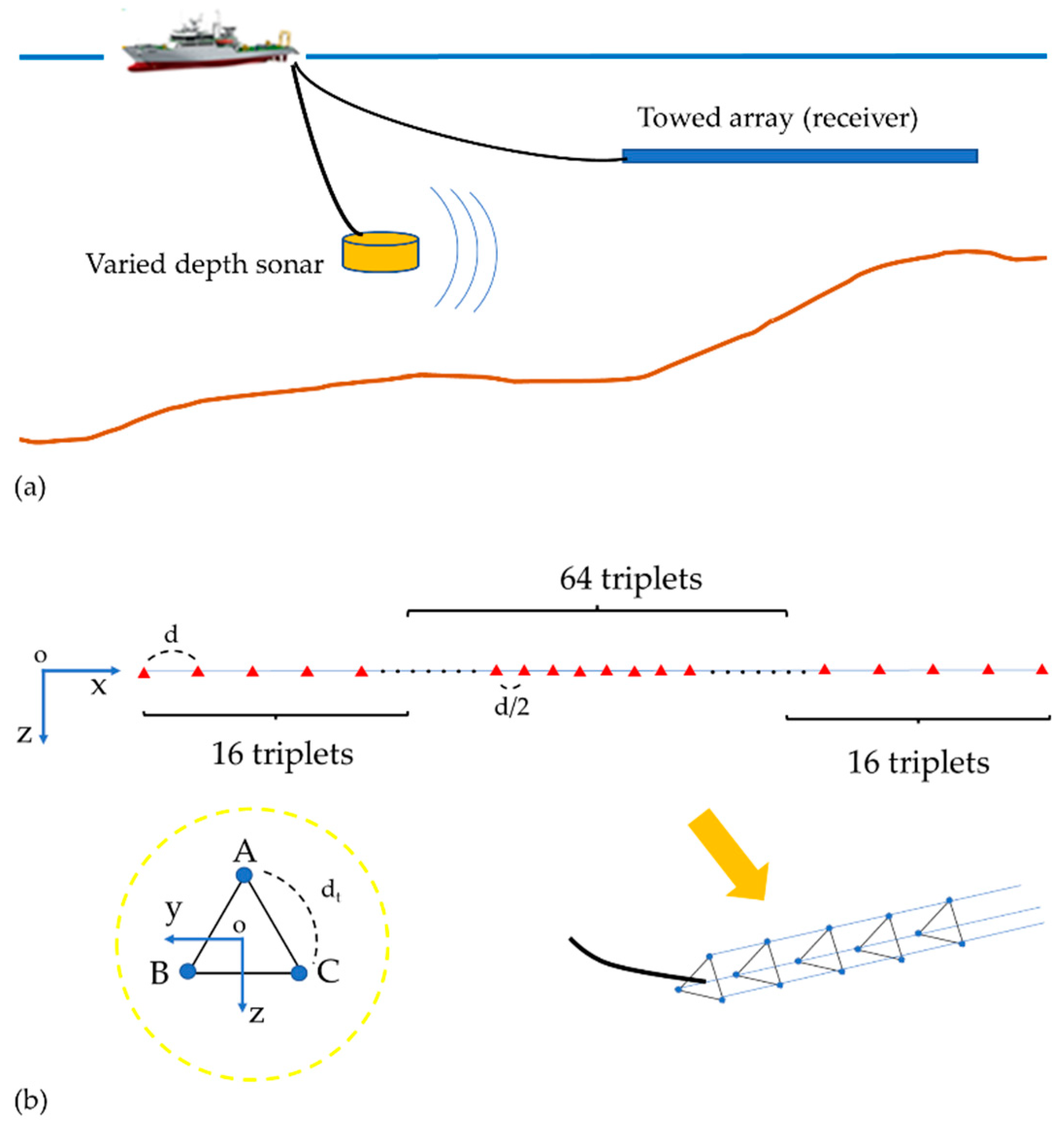
2. ATASS 15 Description

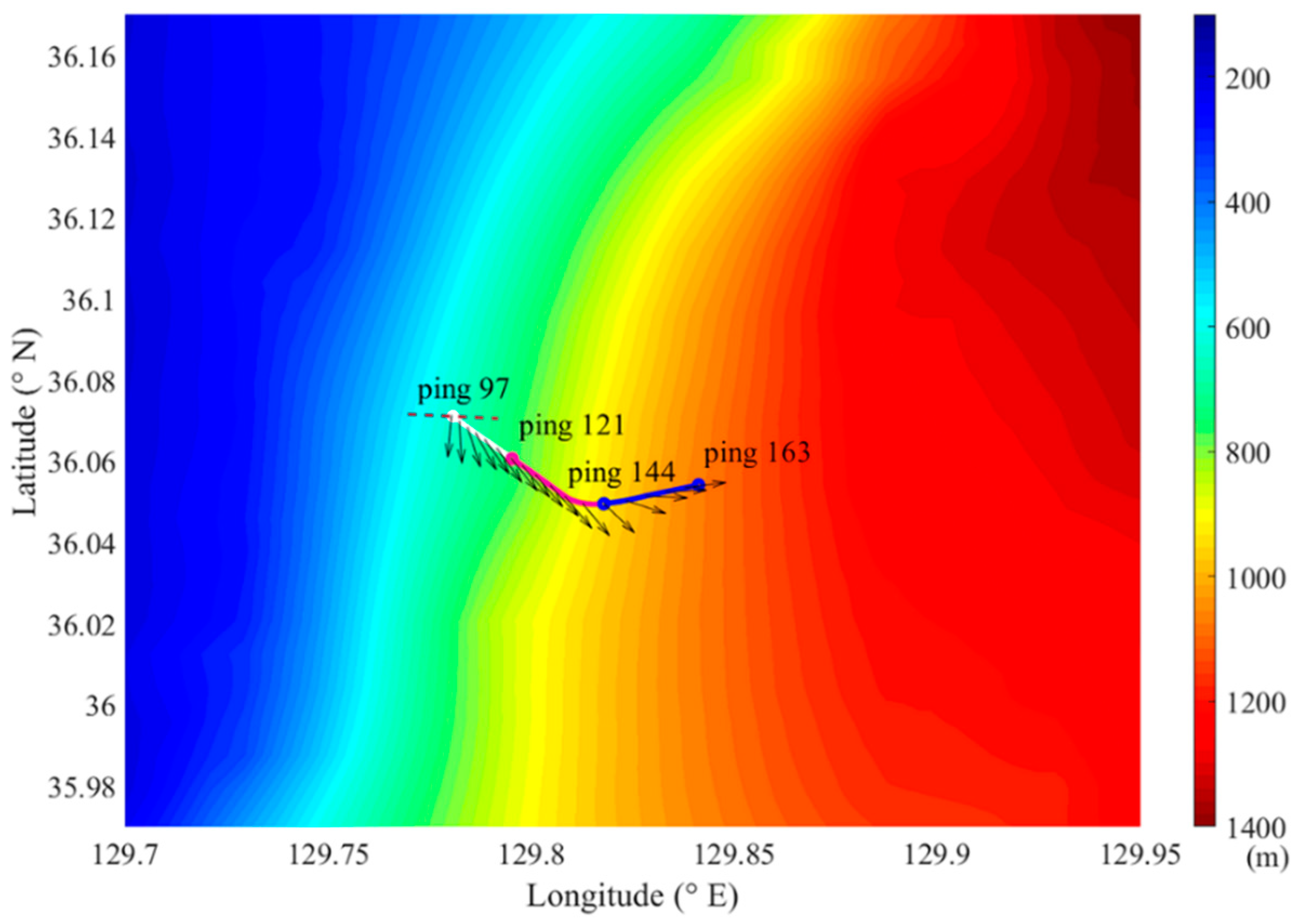
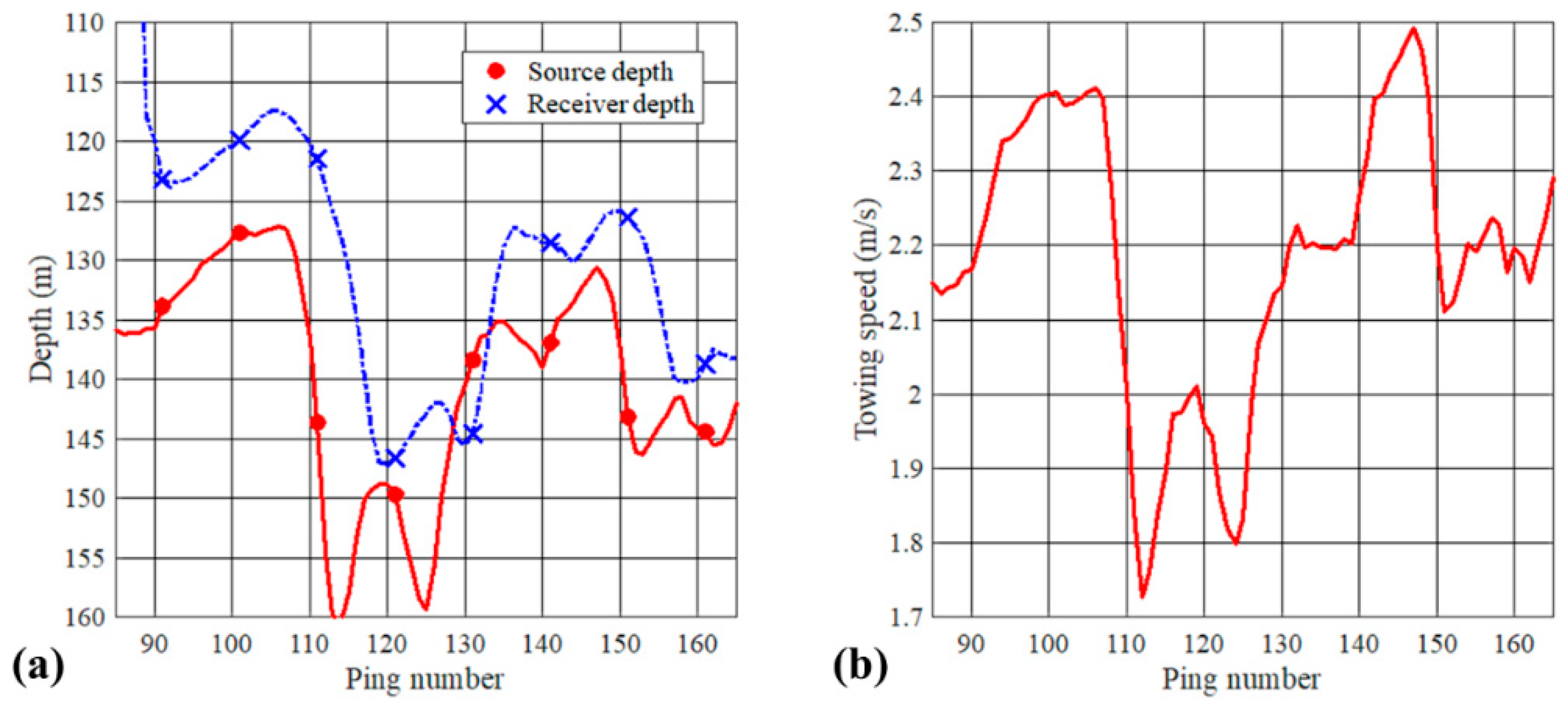
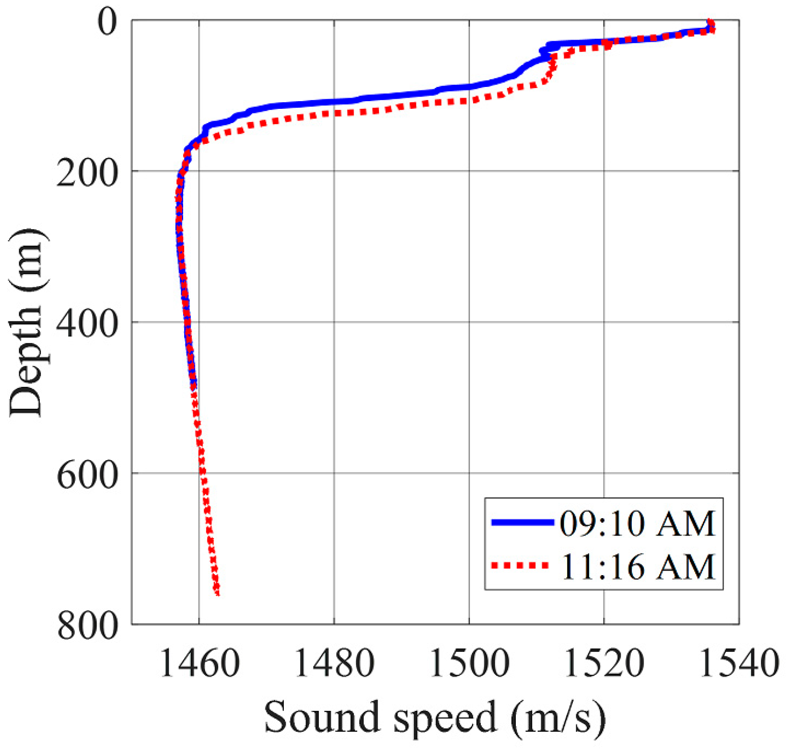
2.1. Experimental Description and Ocean Environment

The ATASS 15 experiment was conducted near the southwestern continental margin of the Ulleung Basin, East Sea, Korea, on 20–21 August 2015 (Figure 1), where the bathymetry was generated from the GEBCO 2020 with a 15 arc-second resolution grid. R/V Cheonghae towed the VDS and the triplet towed array at a speed varying between 1.6 and 2.5 m/s toward the deep ocean. Acoustic transmission signals with a frequency band ranging 1.5–4 kHz were utilized. A total of 678 pings were launched, most of which were CW and linear frequency modulation (LFM) pings. Because the ATASS 15 experiment was conducted for equipment testing of the active array system, a detailed survey of environmental factors was not performed. However, acoustic measurements were accurate under calm sea conditions, and the non-acoustic data of sensor depth, heading, and rolling were recorded in real time.
From 9:06 AM on the first day, the R/V Cheonghae moved southward at a heading angle of 180° measured clockwise from true north, as CW pings were launched for an equipment check-up. At 9:58 AM, the R/V Cheonghae began veering to the east. From this moment to 10:58 AM, the 3 kHz CW transmission experiment was conducted as the R/V Cheonghae moved. The dashed red line in Figure 1 indicates the ship track until 9:58 AM, whereas the solid blue line indicates the ship track until 10:58 AM. The ship tracks were obtained from a global positioning system (GPS) equipped in the towing ship. As shown in Figure 1, the solid blue line crosses the continental slope horizontally, while the green dotted box surrounds the experimental site, which is enlarged in Figure 2.
In Figure 2, the solid lines indicate the track of R/V Cheonghae in the 3 kHz CW experiment and the arrows represent the heading of the towed array at the position of the towing ship, calculated as the average of two compasses equipped in the head and tail of the array. The difference between the two compasses remained below 5°, as the length of the triplet array was small, at approximately 25 m. However, it is noteworthy that the ship heading does not match the array heading in most cases. The circle markers indicate the positions of the ship when changing the pulse length of the CW ping. For visibility, the ping numbers of the four circular markers were added. Pings 1–96 were only used for the initial experimental setup. Information regarding the pulse pings is summarized in Table 1, along with information about the source/receiver depth. Three types of 3 kHz CWs with pulse lengths of 0.1, 0.3, and 1.0 s were used as source pulses. The white, magenta, and blue solid lines in Figure 2 correspond to the A, B, and C cases in Table 1, respectively. The dashed white line indicates the left/right broadside direction of the towed array for the event of ping 97, and the distance between both ends was set to 1 km.
The VDS and towed array were individually cabled to the towing ship. As shown in Figure 3, the towed array was a nested array comprising of 96 hydrophone triplets [1,21], which were divided into three parts: head (16 triplets), body (64 triplets), and tail (16 triplets). A hydrophone triplet consists of three hydrophones arranged as an equilateral triangle with sides of 0.043 m. The 64 triplets in the body part were only used for beamforming and were aligned with the half-wavelength interval with a design frequency of 4 kHz. To monitor the roll motion of the triplets, 18 roll sensors were placed in the towed array.
Meanwhile, the start ranges of the VDS and towed array from the stern varied according to the towing speed and operation depth. In other words, the operation depth is a function of the towing speed and start range. When the towing ship moved in a straight line at a constant speed and the towing cable was assumed to be straight, their values were coarsely tabulated by the manufacturer. For instance, the start range of the towed array was approximately 870 m with an operation depth of 130 m and a towing speed of 4 kn (~2 m/s). At the same towing speed, that of the VDS was approximately 240 m with an operation depth of 150 m. However, during maneuvering, the towing cables would have been bent, and their directions would have not been parallel to the ship’s heading. This caused uncertainty in the horizontal location of the source and receiver, and the operation depths of the source and array were not fixed, but varied constantly between 127 and 161 m, and between 117 and 147 m, as listed in Table 1. This made data analysis difficult and complex. The source depth, receiver depth, and towing speed measured for the 3 kHz CW experiment are plotted in Figure 4.
In the ocean environment, the water temperature and sound speed profile were measured onboard by the XBT at 9:10 AM and 11:16 AM, as shown in Figure 5. Because the maximum depth of the XBT was approximately 760 m, the subsequent profile was extrapolated linearly with depth. The sound speed profile was a typical deep-water profile with a minimum sound speed depth between 226 and 274 m. Because the source was operating close to the ocean surface (<161 m), almost all acoustic intensities formed a downward-refracted beam. At shallow depths, they were reflected at the bottom of the ocean. If the water depth was deeper, some intensities were refracted deeply toward the ocean surface, exhibiting water-borne propagation. Finally, we note that surface reverberation was not considered in this study because the sea was calm, and no remarkable recording was found in the reverberation data.

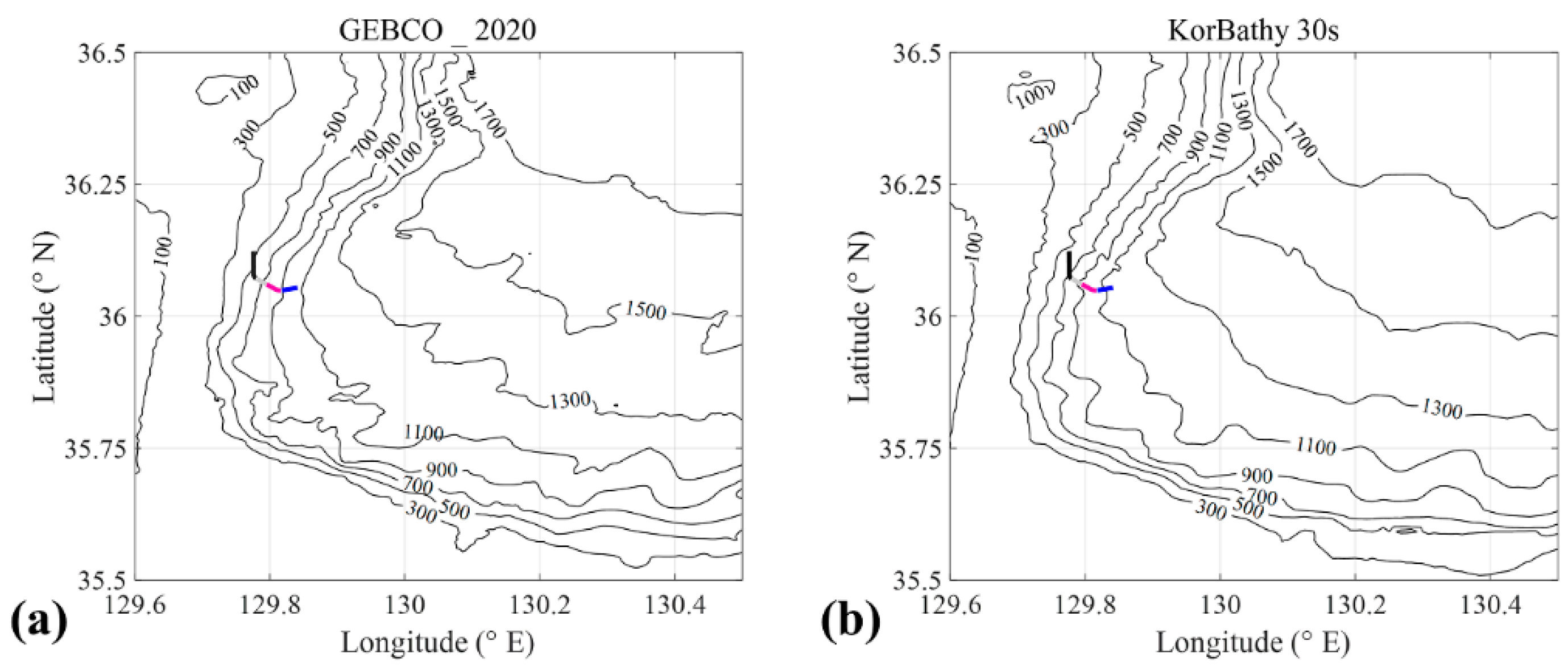
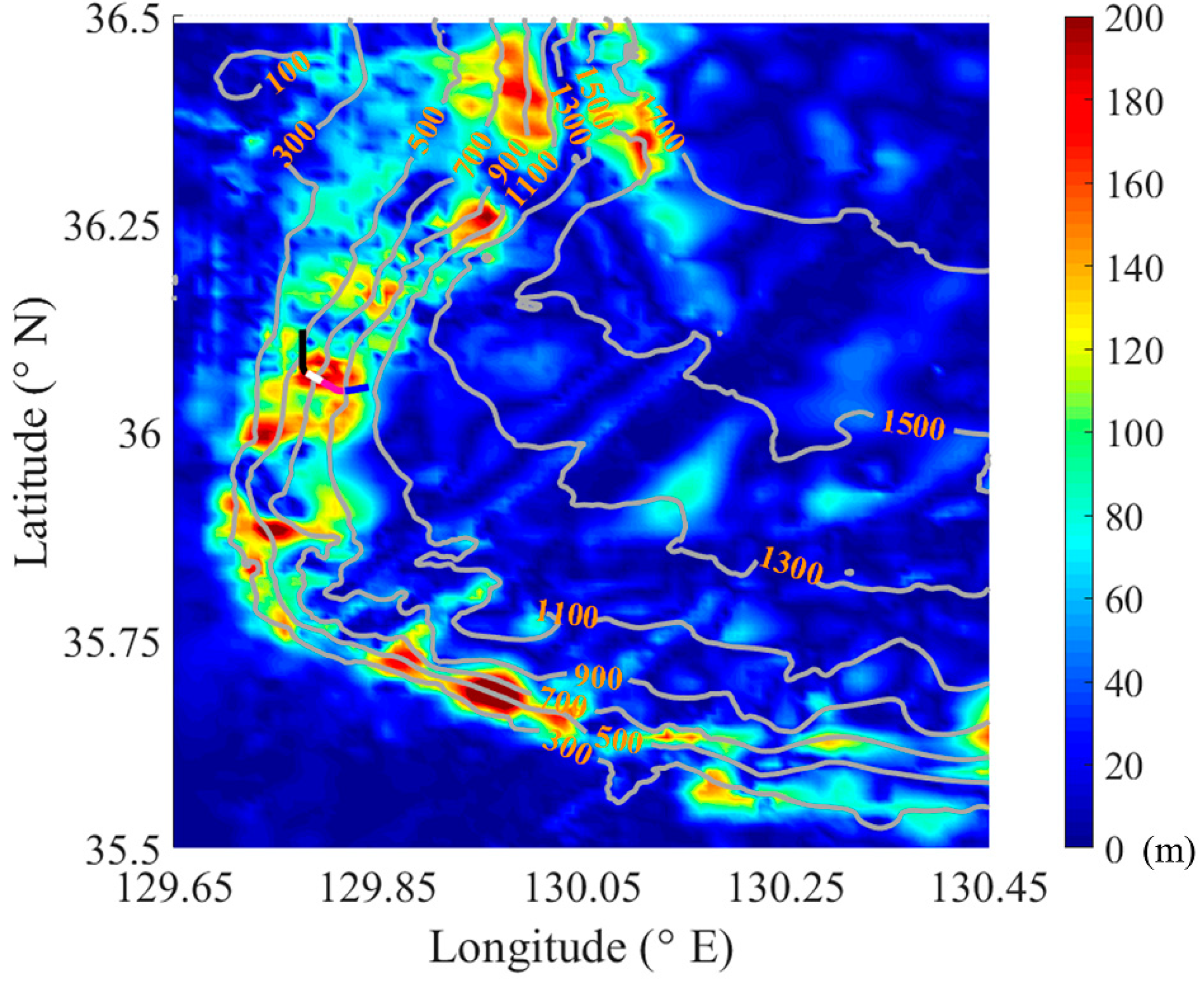
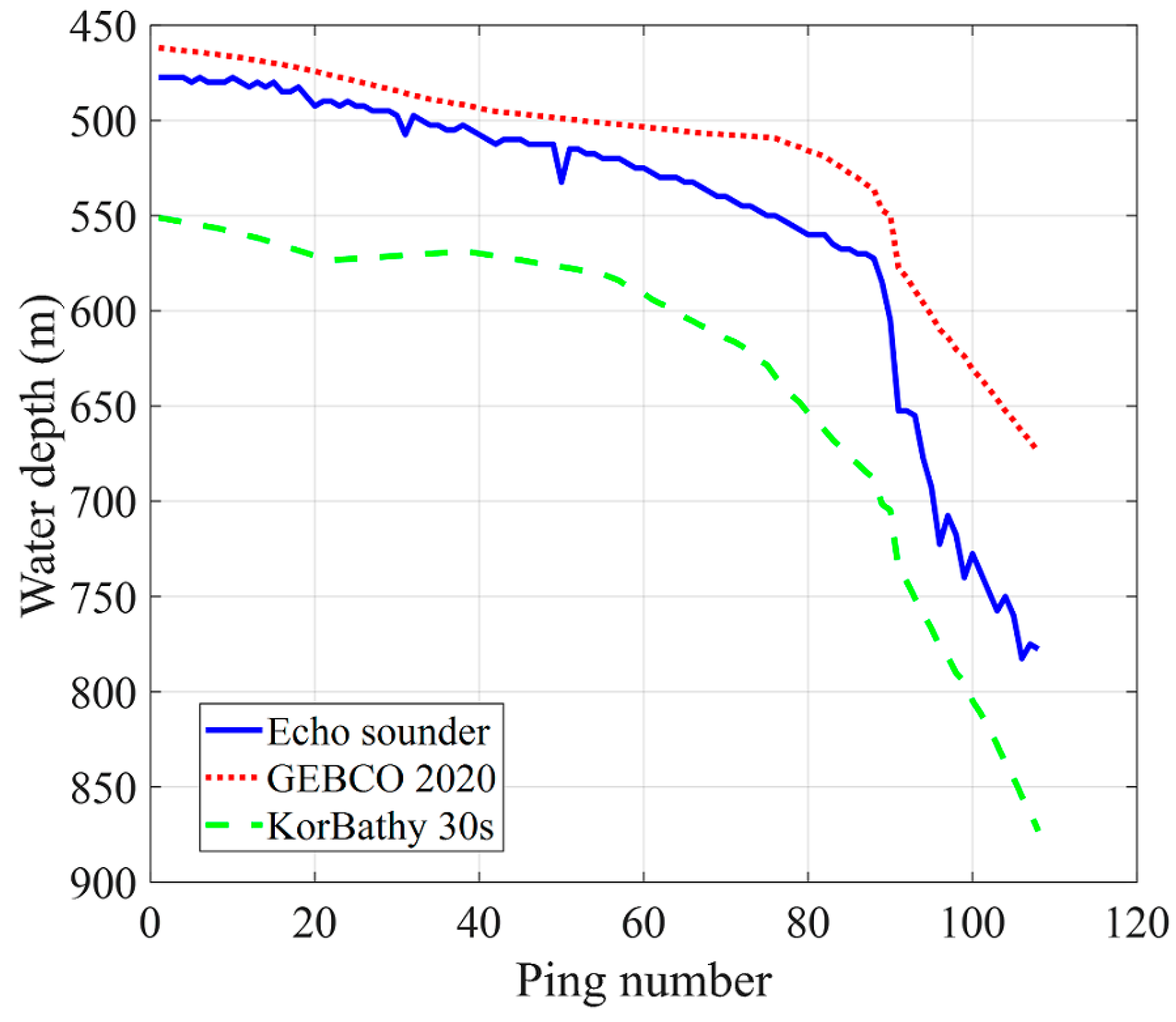
2.2. Bathymetry and Geoacoustic Modeling

As shown in Figure 1, the experimental site spans the outer continental shelf and continental slope and is connected to the southwestern part of the Ulleung Basin of the deep, bowl-shaped back-arc basin in the East Sea [19,20,21,22]. The bathymetry is range-dependent, where the water depth varies from 100 to 1500 m. Since the mid-1980s, a few geological studies and geotechnical surveys have been conducted to investigate the stratigraphy and morphology of the continental margin. It was found that the mass-movement deposit dominated along the entire margin of the Ulleung Basin, overlaid by hemipelagic mud.
In 2013, Kim [23] acquired 157 core samples obtained from different points from a latitude of 35° to 36° and a longitude of 129° to 131° (Figure 1) and constructed a geoacoustic model for the southwestern continental margin. Because their work was only published in Korean, we concisely provide readers with their results in this section. They analyzed 71 piston core samples with linear lengths of 8 m, 20 piston core samples with linear lengths of 4 m, and 66 box core samples. Based on the sediment texture of the core sample and the p-wave measurement in the laboratory, the southwestern continental margin was divided into five geoacoustic provinces. Among these provinces, our experimental site was located in the province with hemipelagic mud partially mixed with intermittent sandy sediments originating from the outer continental shelf due to slide/slump or turbid flow. Although the sediment thickness was not explored in their work, other studies [18,19,24,25,26] that used seismic profiling reported that the sediment thickness varied from a few meters to several tens of meters in the margin of the Ulleung Basin, and the sediment thickness was significantly affected by the slope stability. Acoustically, the effect of the thickness will be more pronounced in the low-frequency range, but it will be negligible at a 3 kHz frequency.
From the core samples, the laboratory p-wave speed was measured in the range of 1481–1512 m/s at room temperature. The laboratory p-wave speed was corrected using the empirical model proposed by Kim [27] and the geoacoustic model of Hamilton [28] using the velocity ratio, water temperature in the sediment, depth, and salinity. The corrected in-situ p-wave speed was predicted to range from 1411 to 1458 m/s for Kim’s empirical model and 1440–1460 m/s for Hamilton’s geoacoustic model [29]. Because these values in the sediment are lower than the water sound speed on the sea floor, the sediment at the experimental site is acoustically slow and can be considered as a soft bottom (or soft sediment). A soft bottom results in a small reflection and a large bottom loss. Therefore, when the beams propagating along the 1/2 CZ path interact with the ocean bottom, the intensity of the reflected beams is reduced significantly.

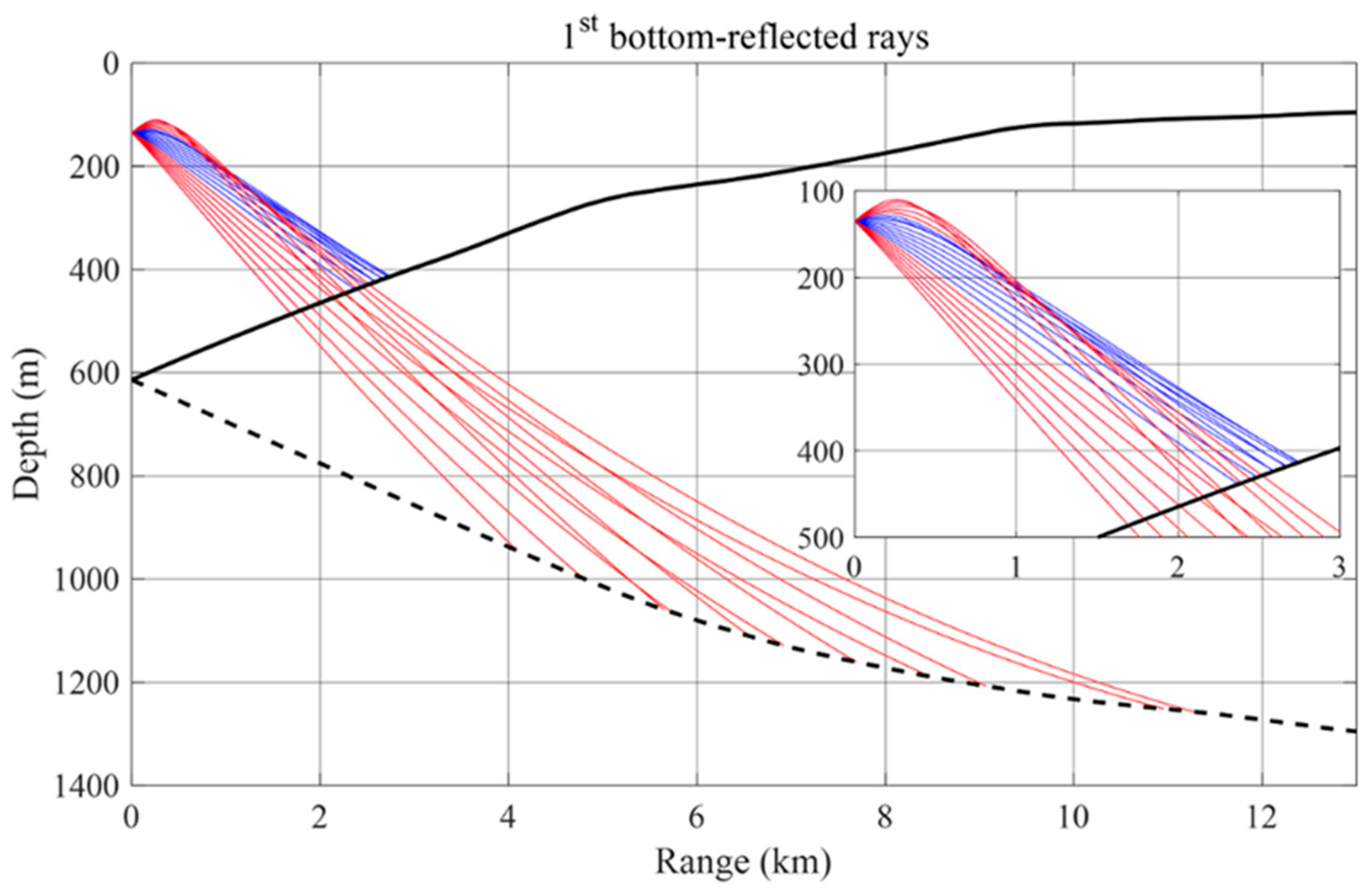
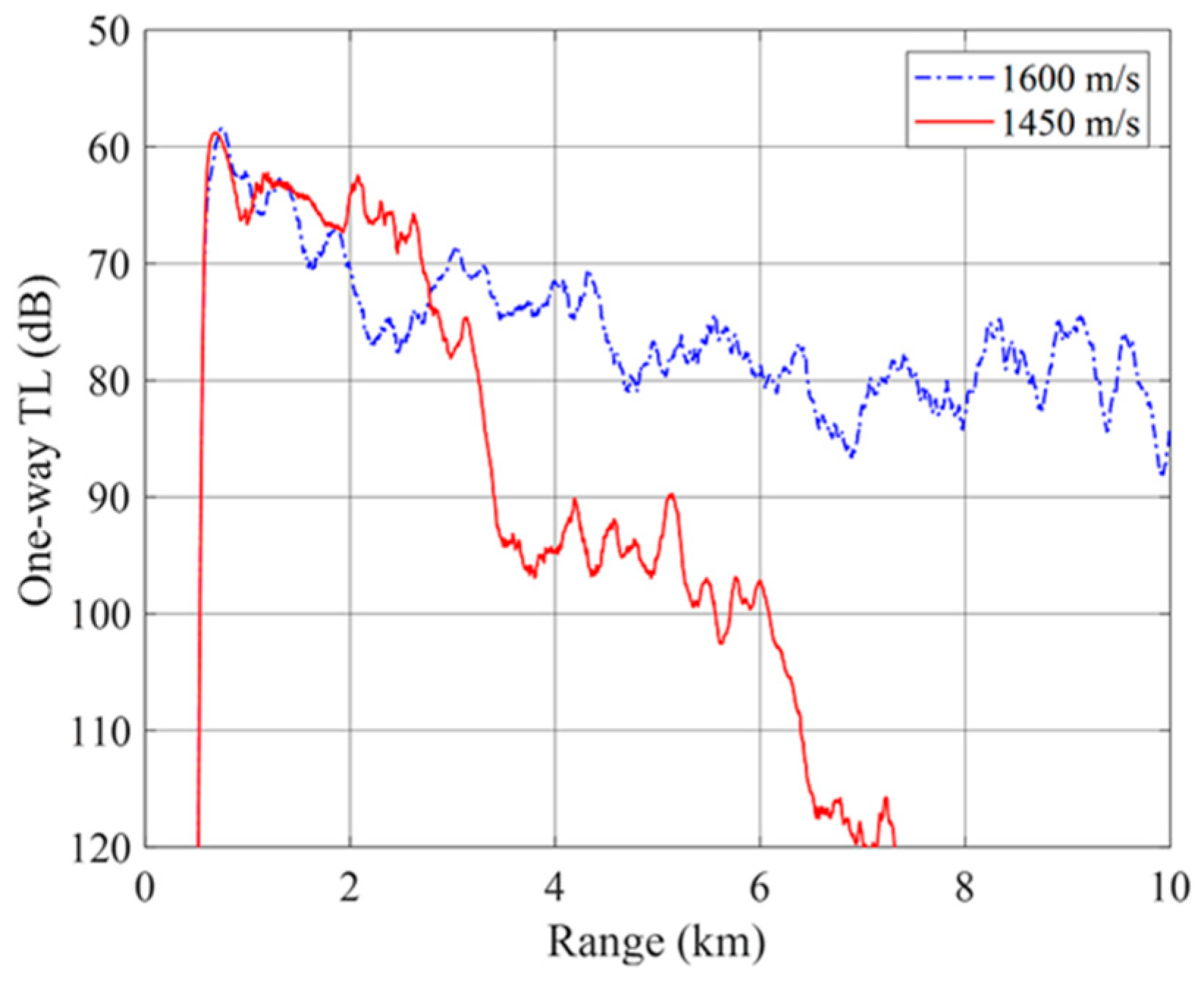
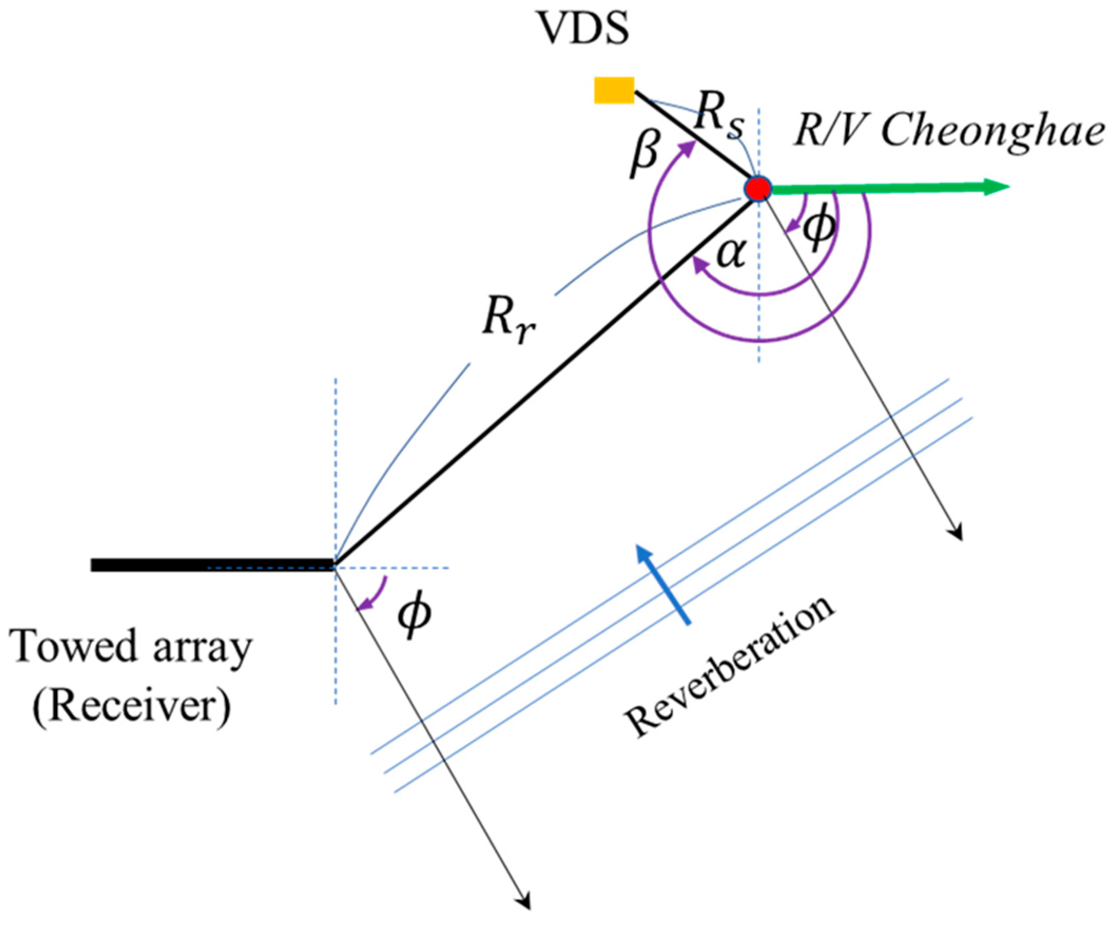
2.3. Structure of Acoustic Propagation in Water

To demonstrate the acoustic propagation in the ocean environment described above, we first modeled the geometrical ray structure with the sound speed profile as shown in Figure 5. The source depth was set to 135 m at the ship position at approximately ping 97, based on the data in Table 1. The speed of sound at the source depth was 1467 m/s. The corresponding conjugate depth was 1014 m. For a bathymetry depth smaller than the conjugate depth, the downward-refracted rays must interact with the bottom. However, at deeper bathymetry depths, they are partially reflected or propagated along the CZ path.
A similar analysis was performed by Makris and Berkson [6] in the ocean environment of the western flank of the Mid-Atlantic Ridge. This site had a mean depth of 3785 m, which was assumed to be a fast bottom. The source frequency was 270 Hz, and the scale of the experimental area was approximately 200 km × 200 km. They found that the strong backscatter is the result of the rugged bathymetry in the (n + 1/2) CZ range, where a water-borne path is available. However, the 3 kHz reverberation in our work was not generated by large-scale roughness such as ridges. As shown in Figure 2, the bathymetry depth of the experimental site increased or decreased almost monotonically at an azimuth angle.
Figure 6 shows the results of the geometrical ray tracing. The fan angle was set between −10° and 10° at 1° intervals. The solid and dashed black lines correspond to two bathymetries cut at the right (90°) and left (270°) of the towed array heading, and they are superimposed. The blue and red solid lines indicate the ray trajectories. The blue solid lines represent the rays, which are reflected from the upslope bathymetry, but form the water-borne path for downslope bathymetry. The red solid lines are the bottom-reflected rays for both the upslope and downslope bathymetries. Because the bottom is slow and the impedance difference between water and sediment is low, we anticipate the subsequent multiple bottom-reflected paths to be much weaker.
To examine the amplitude of the wave field, a range-averaged one-way transmission loss between the source and bottom cell was simulated using the parabolic equation model for soft (mud) and hard (sand) bottoms. The upslope bathymetry of Figure 6 and the sound speed profile in Figure 5 were used. The soft and hard bottom sound speeds were set to 1450 m/s and 1600 m/s, respectively. The bottom density and attenuation were 1.331 g/cm3 and 0.1 dB/λ, respectively, in both cases. The source depth was 135 m. As shown in Figure 7, the transmission loss of the hard bottom gradually increased in the range. However, the transmission loss of the soft bottom increased sharply after the first bottom hit. This implies that the multiple bottom-reflected paths for the soft bottom were much weaker than the insonified fields. Therefore, stronger reverberation is limited within the region where the first bottom hit of water-borne paths occurs, which is often known as the direct path area. Thus, we defined the maximum direct path (MDP) range as the limit of the direct path area. The MDP range was predicted through ray tracing, as the sound speed profile and bathymetry were provided. In addition, the MDP range was easily checked by the transmission loss between the source position and the bottom cell of the sea floor.
To confirm the MDP range in the spatially varying bathymetry, the two-way transmission loss between the source, receiver, and bottom cell was calculated using the parabolic equation model at the ship positions for pings 97 and 144. We used the source and receiver depths as the measured values for each ping (see Table 1). The bottom had a sound speed of 1447.5 m/s, a density of 1.331 g/cm3, and an attenuation of 0.1 dB/λ.
Figure 8a,b show the bathymetry map as a function of the range and relative azimuth angle, which is defined clockwise from the array heading. Note that the position for ping 144 was deeper, as shown in Figure 2. Figure 8c,d show the two-way transmission loss for each ship position. In the short range, where the high grazing rays are dominant, the transmission loss was very large for all azimuth angles. The region in the longer range is visually divided into two areas: direct and multiple path areas. Their boundary, which resembles a bathtub curve, represents the MDP range curve. Comparing the transmission loss with the bathymetry, it can be observed that the downslope and deep bathymetry depths cause a longer MDP range. As the bathymetry depth is deeper than the conjugate depth, the water-borne waves interact with the bottom further away. Conversely, the MDP range is shortened for upslope and shallower bathymetry depths [30,31].
Accordingly, the shape of the MDP range curve was different for bathymetry at the source position. The width of the curve in the azimuth angle was narrower for the source in the deeper sea (ping 144). This is because the upslope and shallow bathymetry depths are limited to a narrow azimuth angle. Within these restricted azimuth angles, the direct downward-refracted rays completely interact with the ocean bottom. The amplitude of the backscatter may also be of interest, as it depends on the scattering area and the bottom scattering strength. A comparison of the modeled and measured reverberation was provided in our previous study [2] under the assumption of a depth-bistatic geometry. However, this topic will not be considered here because it is beyond the scope of this study.

3. Results and Discussion

3.1. Triplet Array Beamforming

The BTR for CW ping was obtained through conventional time-domain beamforming of the measured data. The steering angle is uniformly divided into the domain of cos (∅) with the azimuth angle ∅. The total number of angle bins was 128. These conditions yield a finer beam resolution on the broadside. The beamformed signals were transformed into baseband signals using Hilbert transformation and low-pass filtering. Note that all the figures in this paper are processed based on the baseband signal.

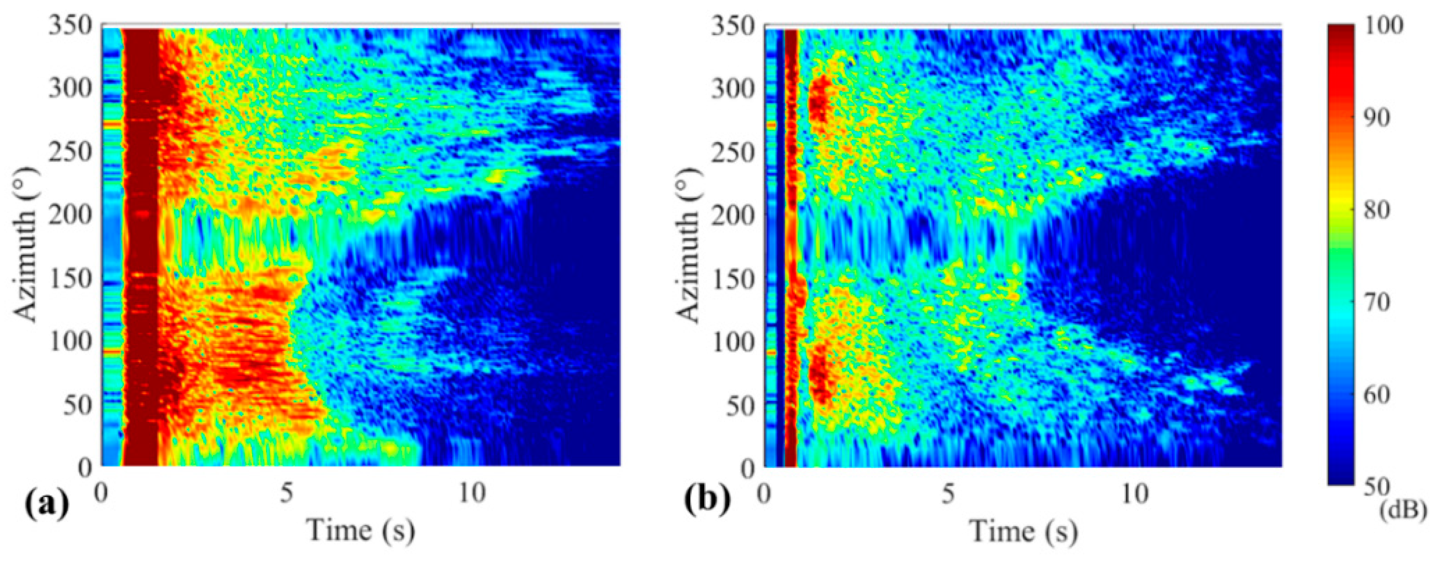
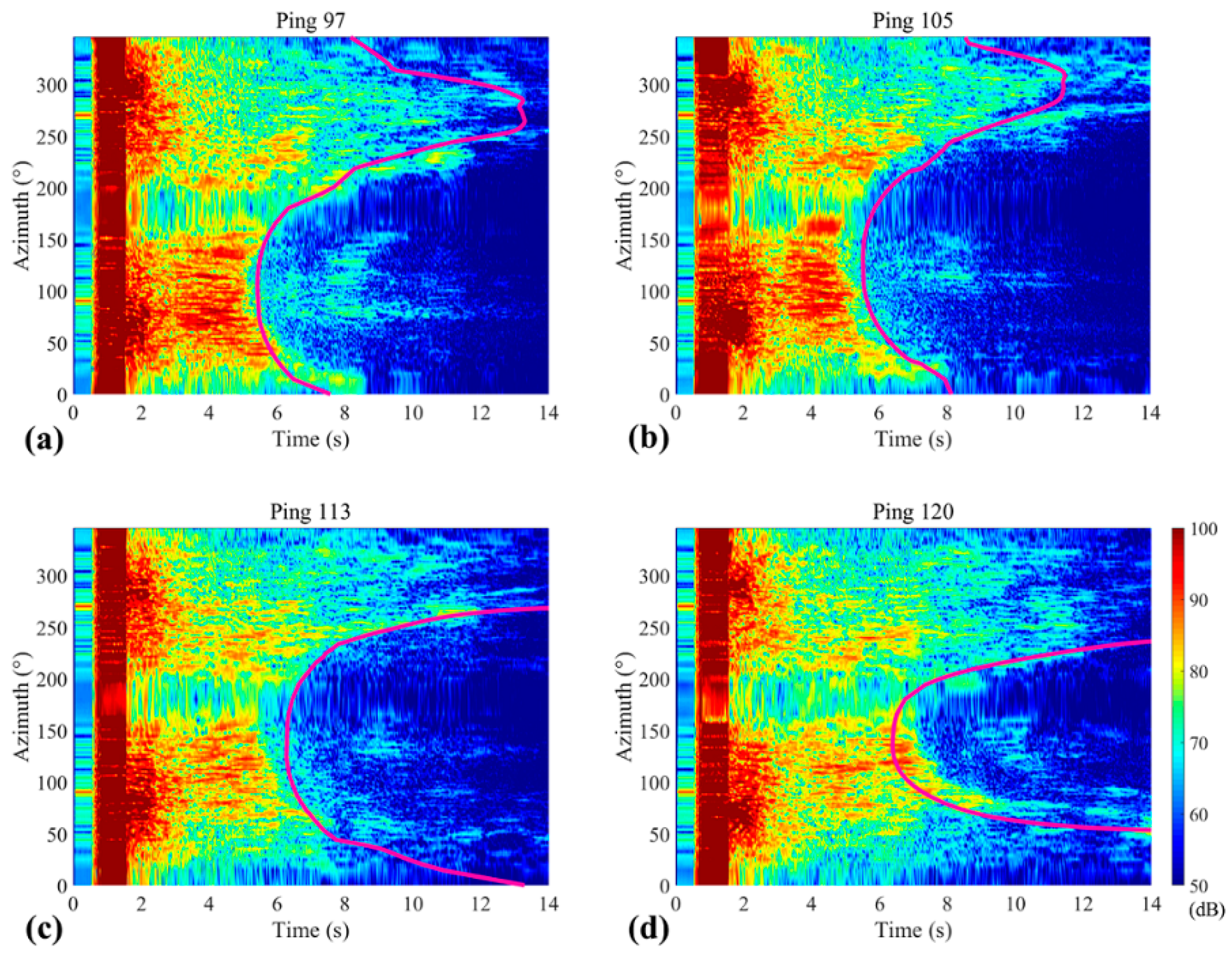
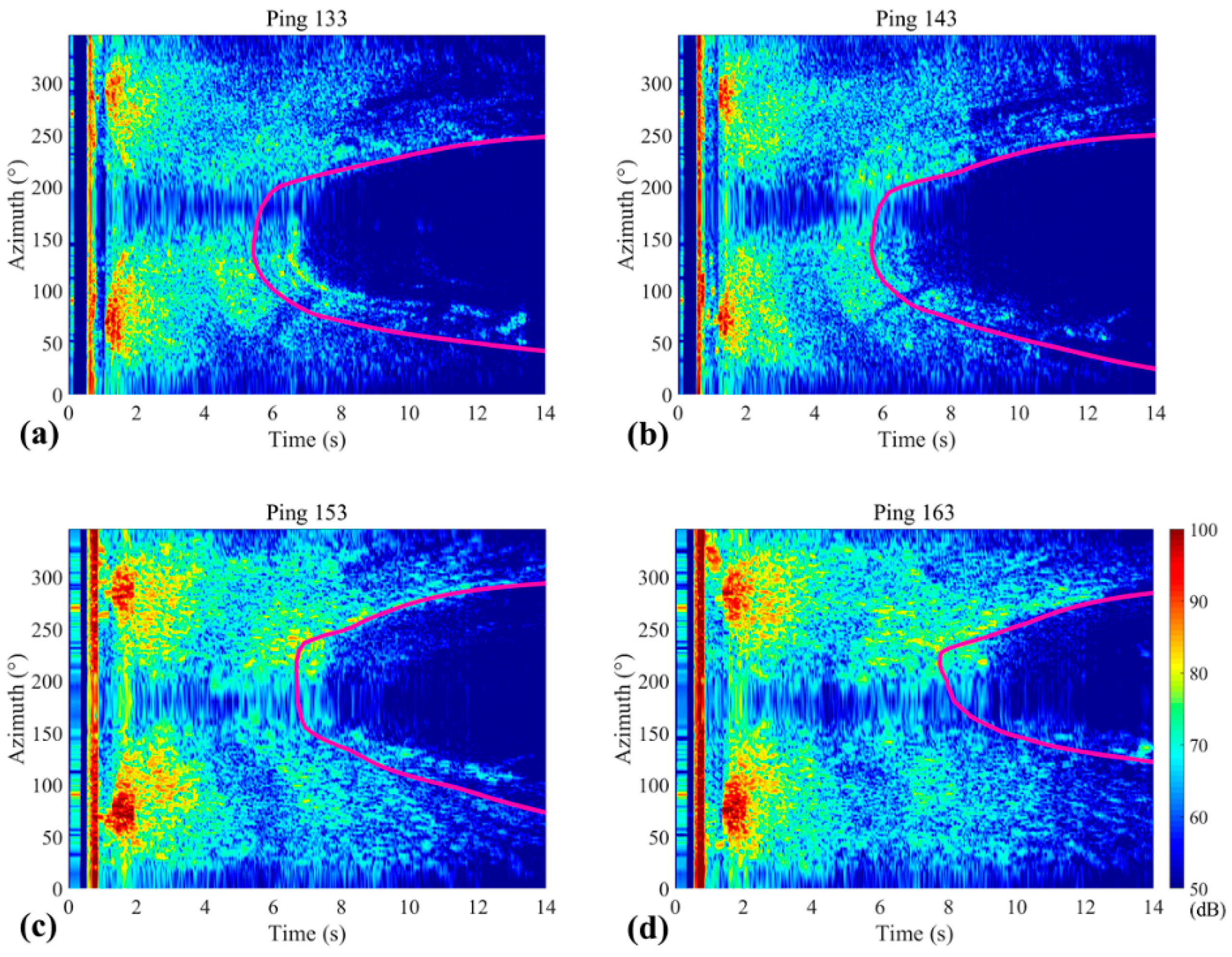
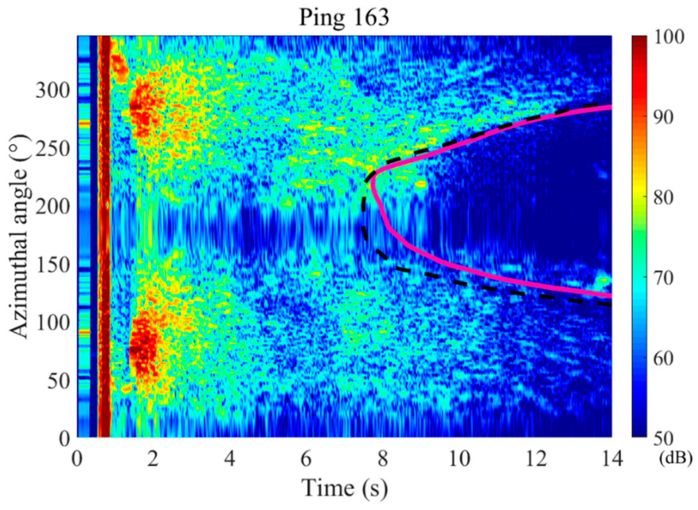
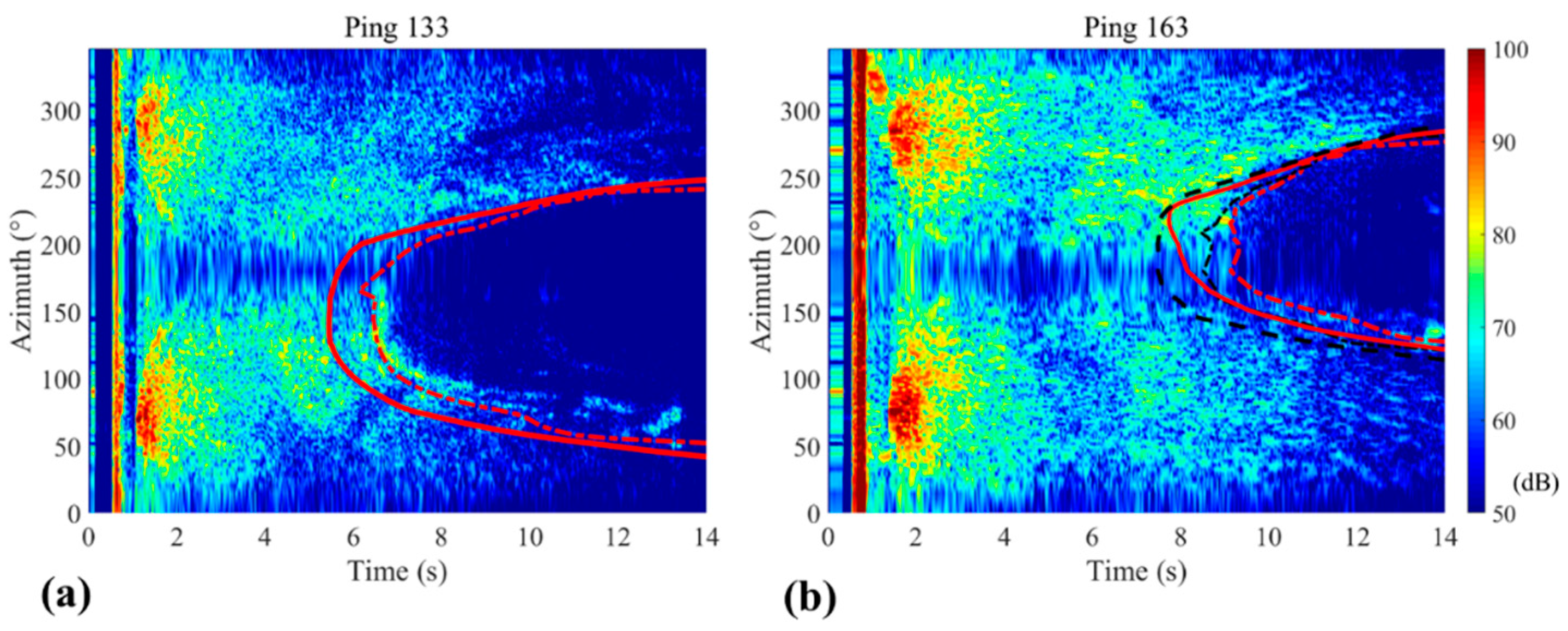
3.2. Bearing-Time Record Pattern
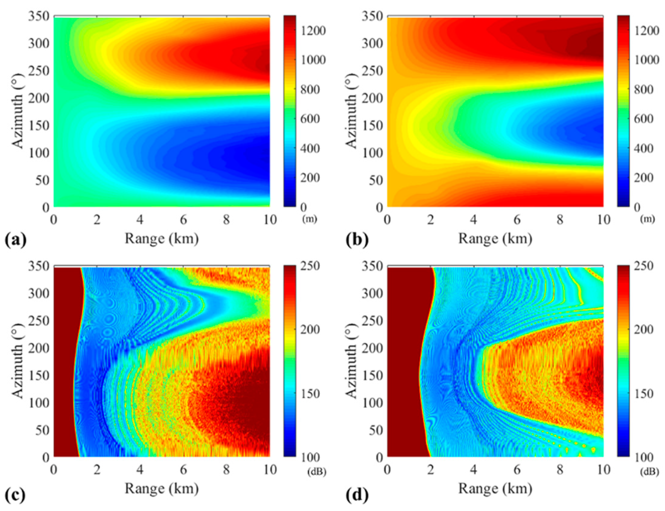
In Figure 9a,b, the BTRs for pings 97 and 144 are plotted corresponding to the 3 kHz CWs with pulse lengths of 1 and 0.3 s, respectively. The x-axis represents the relative azimuth angle, which was measured clockwise from the array heading direction, whereas the y-axis represents time, where the time origin corresponds to the ping launch time. As shown in the transmission modeling, we also observed a drop-off region of reverberation in the time-azimuth domain (the travel time is simply related to the range with the reference sound speed). Clearly, the contour at the boundary resembles a bathtub. We reported that such a bathtub pattern occurred in all CW data measured on the continental slope, although the shape differs slightly depending on the position of the ship. As shown in Figure 9, the signal that arrived early with the highest level is a direct blast, the amplitude of which was clipped for system protection, and which was used to estimate the distance between the source and the array. Additionally, in Figure 9a, some moderate reverberation intensity is observed at 8 s within the azimuth angle range of 80–130°. This is caused by the second bottom-reflected waves. Their amplitudes were more than 30 dB lower than those of the first bottom-reflected waves.

3.3. Simulation

To quantify the observations described in the previous section, we simulated the interface between the stronger reverberation region and the drop-off region, known as the two-way MDP travel time in this study, through N×2D geometrical ray modeling. The two-way MDP travel time is defined as the two-way travel time from the source to the bottom in the MDP range and from the bottom in the MDP range to the receiver.
This problem is basically a bistatic configuration, as shown in Figure 10, because the source and receiver are separated. To reflect on the bistatic geometry, four unknown parameters, which vary during a turn, are required: two distances, between the R/V vessel and the source and between the R/V vessel and the receiver, and two azimuth angles. However, owing to incomplete information on the horizontal location of the source and receiver during a turn, the fully bistatic model will have significant uncertainty and thus can result in the overkill approach. Fortunately, the depth of the source and receiver was recorded during the experiment. In these situations, a depth-bistatic approach is an appropriate choice for the first-order modeling of the two-way MDP travel time. In this study, we mainly used the depth-bistatic approach. Later, full bistatic modeling will be applied to the case of ping 163, for which the configuration of the source and receiver array might be estimated.
For depth-bistatic modeling, we assume that the source and receiver are located at the GPS position of the R/V vessel in the range and azimuth angle. At this GPS position, the bathymetry along a 20 km radius was removed at 128 relative azimuth angles. For each bathymetry, the two-way direct path travel times between the source, receiver, and bottom cells were computed through ray tracing in an evenly spaced horizontal range, and the two-way MDP travel time was determined as the maximum value at the corresponding bathymetry. Through repetitive computation, the two-way MDP travel time at the ship position was obtained as a function of the relative azimuth angles. Additionally, it is emphasized that two-way MDP travel time modeling is much faster than the full reverberation modeling, which overcomes the lack of environmental properties for bottom reverberation. The full bistatic modeling is similar to depth-bistatic modeling, except that the horizontal locations of the source and receiver array are different. The bottom cells were divided based on the coordinates of the receiver. To increase the accuracy of bistatic modeling, linear interpolation was applied in the calculation of one-way MDP travel time between the source and bottom cell.
We applied the above procedure to all 67 CW ping events and obtained 67 curves for the two-way MDP travel time. Eight representative results are shown in Figure 11 and Figure 12, overlaid with the BTR. The solid magenta line indicates the curve of ‘the two-way MDP travel time plus pulse length’, referred to as the ‘two-way MDP travel time+’ in this study. The BTRs in Figure 11 have a pulse length of 1 s. In Figure 12, the upper part shows a pulse length of 0.1 s, whereas the lower part shows a pulse length of 0.3 s. These figures show agreement between the two-way MDP time+ and the observed BTR pattern. As the ping number increased, the width of the curve narrowed. This is because azimuth angles with a short MDP range become more restricted as the R/V vessel moves deeper into the sea.
Based on the towed array heading in Figure 1 and Figure 2, the above eight results are divided into three groups (not to be confused with the groups categorized in Table 1). The first group consisted of pings 97 and 105. Thereafter, the arrays were approximately set toward the south, and the bathymetry depths were below 700 m. Pings 113, 120, 133, and 143 formed the second group. Their array headings varied from 144° to 138° clockwise from the true north. The bathymetry depths were approximately 700–900 m. The last group consisted of ping 153, with an array heading angle of 91°, and ping 163, with an array heading angle of 83°. While turning from south to east, the towing speed and source/receiver depths varied significantly, as shown in Figure 4. This implies that the horizontal locations of the source and receiver also fluctuated until the turn is over. A careful examination of Figure 11 and Figure 12 reveals that there is some discrepancy between the modeled curve and the BTR patterns. In particular, for the azimuth angle between 70° and 160°, the pings of the second group displayed strong reverberations inside the bathtub. Such leakages also appeared in the third group of pings 153 and 163 in the azimuth angle between 200° and 240°. In all 67 results, these discrepancies were observed equally in the BTRs of the same group.

3.4. Discussion

To explore the origins of these discrepancies, we considered three environmental factors affecting the pattern of BTR: the range and azimuth-dependent sound speed profile, the limitation of depth-bistatic modeling, and the bathymetry. As previously mentioned, the sound speed profiles (SSP) were only measured with the XBT along the direction of the towing ship. As shown in Figure 4, the sound speed profile varied in the thermocline over time. However, the magnitude of the change was not sufficiently large to distort the 1/2 direct path. It is also unlikely that the SSP significantly varies with the azimuth angle within a radius of ~10 km. Therefore, the spatial variation of the SSP does not seem to be the main cause of the discrepancies.
Second, we considered the limitations of the depth-bistatic modeling. Our two-way MPD time+ curves were obtained under the assumption of a depth-bistatic configuration. We examined the arrival time of a direct blast at the first hydrophone in a triplet array line. During the experiment, the arrival time of the direct blast ranged approximately from 0.5 to 0.52 s, corresponding to distances of 734 to 763 m, respectively, with a reference sound speed of 1467 m/s. Given that the difference between the source and receiver depths is small, the distance approximately corresponds to the horizontal distance between the source and receiver.
To check the limitation of depth-bistatic modeling, full bistatic modeling was performed with the ocean environments of ping 163. In this case, considering that the ship direction is similar to the array direction, as shown in Figure 2, we inferred that the two azimuth angles (α and β) of Figure 10 are close to π, which indicates that the ship, source, and receiver array are in a straight line. The distance between the R/V vessel and the source and between the R/V vessel and the receiver were approximately determined from the manufacturer’s table as 196.2 m and 916.8 m, respectively.
As shown in Figure 13, we compared the results of the full bistatic modeling with those of depth-bistatic modeling. It can be observed that full bistatic modeling yields a slightly different result. The two-way MDP time arrivals near the relative azimuth angle of 180° were shorter. Note that this curve can be tuned by changing the configuration of the source and receiver. Nevertheless, it is impossible to account for the difference between the two-way MDP time+ and the observed BTR pattern from bistatic modeling alone.
Finally, we examined the fitness of the bathymetry model of GEBCO 2020, a global terrain model for ocean and land with a grid spacing of 15 s in latitude and longitude, which is widely used worldwide for general purposes. For comparison, another set of bathymetry data were taken from KorBathy 30s [32], which is a domestic model with a resolution of 30 s in latitude and longitude, based on gridded data of 1 min and the digital nautical charts issued by the Korea Hydrographic and Oceanographic Agency, developed in 2007. Figure 14a,b show the contours of the two bathymetry models at the experimental site. The contour lines of GEBCO 2020 were plotted using the interpolated data from coordinate points in the KorBathy 30s for comparison on the same basis. As shown in Figure 14, GEBCO 2020 seems to display more detailed topographic features than KorBathy’s 30s.
Figure 15 shows the absolute difference between GEBCO 2020 and KorBathy 30s. Significant differences were observed in the continental slope of the Ulleung Basin, where the experiment was conducted. To further investigate the effect of bathymetry, the BTR curves were once again modeled for two typical pings (pings 133 and 163) in the depth-bistatic geometry with the bathymetry data of the KorBathy 30s. For the case of ping 163, full bistatic modeling was also performed.
Figure 16 shows the BTR curves based on KorBathy 30s (red dash-dotted line) which show better agreement with the pattern of the measured BTR when compared with Figure 12, which is based on GEBCO 2020. This is because the domestic model reflects more echo sounder data on the continental slope of the Ulleung Basin, although it has a lower resolution. As shown in Figure 16b, the two results of the full bistatic modeling with the KorBathy 30s and the GEBCO 2020 were added. This shows that employing KorBathy 30s produces more reasonable results. Interestingly, the results of the full bistatic modeling are not the most accurate. This may either be because the uncertainty of bathymetry still exists, or because the four input parameters used in the bistatic configuration are not accurate. Improvements in the simulation accuracy can be achieved in the future with new data collected by a well-organized experiment with a high-resolution, bottom survey, and precise sensing of sonar configuration.
In addition, we analyzed the echo sounder data of a towing ship. These data were collected at ship positions ranging from 1 to 108. As shown in Figure 17, we compared the echo sounder data with two bathymetry models for the ‘ping number’ corresponding to the position of the ship. Although there is no exact match, the echo sounder data are closer to the data of KorBathy 30s over ping 91, but follow the data of GEBCO 2020 at a lower ping number. This tendency was consistent with our hypothesis. Therefore, it is considered that the initial discrepancies between the two-way MDP time+ and the observed BTR pattern were mainly caused by the inaccuracy of the bathymetry, and the use of the KorBathy 30s provides more confident results near the continental slope of the Ulleung Basin, East Sea.

4. Conclusions

We presented the analysis of 3-kHz CW reverberation measured in the southwestern continental margin of the East Sea using an active triplet towed array. During the experiment, the towing ship moved south along the continental shelf and turned east toward the deep sea. The 3-kHz CW measurements were performed during the turn. In the bearing-time records of the reverberation signal, we observed a drop-off region, which varied as the towing ship moved toward the deep sea. Using a geological literature survey and propagation modeling, we demonstrated that such a pattern is caused by the interaction of a direct ray along the 1/2 CZ path with the soft bottom.
For a more precise analysis, we modeled the boundary of the drop-off region using an N×2D ray tracing model under the assumption of a depth-bistatic configuration. The modeled curves, known as the two-way MDP travel time curves in this study, moderately correspond to the boundary pattern of the drop-off region in the BTRs. However, we observed significant differences between them, which were primarily caused by the inaccuracy of the bathymetry model of GEBCO 2020 on the continental slope. We showed that the biases can be reduced by using a domestic bathymetry model known as KorBathy 30s. The secondary cause of the inaccuracy may be the limitation of depth-bistatic modeling as, although it can approximately identify a drop-off region in the BTR, it is only a crude approximation of the bistatic configuration. However, in the case of ping 163, the use of full bistatic modeling did not yield optimal results. This is because there was still some ambiguity regarding the bathymetry and bistatic configuration.
Finally, we focused on the observed BTR pattern in this study, which depends on the sound speed profile, bathymetry, and source–receiver configuration. Thus, it can provide additional information in the absence of one of these pieces of information; for instance, environmental parameter estimation with acoustic signals, self-localization of a large underwater vehicle in an emergency using the BTR and map, or conditioning the source–receiver operation. In this study, we faced numerous difficulties in obtaining information about high-resolution bathymetry/geoacoustic models and towing cable dynamics, because this reverberation experiment was not designed for basic study. In the future, the acquisition of high-resolution environmental data will be of great significance in understanding the BTR bathtub pattern in detail using the best prediction model.

Author Contributions

Conceptualization, Y.J. and K.L.; methodology, K.L.; data processing, Y.J.; writing—original draft preparation, Y.J. and K.L. All authors have read and agreed to the published version of the manuscript.

Funding

This study was supported by the National Research Foundation of Korea (NRF), grant-funded by the Korean government (MSIT) (No. 2019R1F1A1059146), and the Agency for Defense Development (ADD) Republic of Korea (No. UD190005DD).

Institutional Review Board Statement

Not applicable.

Informed Consent Statement

Not applicable.

Acknowledgments

We would like to thank Byung-Nam Kim (Korea Institute of Ocean Science and Technology) and Sung Yong Kim (KAIST) for providing information on the ocean environment at the corresponding site, and Woojae Seong (SNU) for his good comments and discussions. Also, we would also like to thank Young-woo Ryu and Jungyong Park (ADD) for their contributions to acoustic and marine equipment.

Conflicts of Interest

The authors declare no conflict of interest.

References

  1. Lee, K.; Seong, W.; Kim, S. Estimation of the roll angle in a triplet towed array using oceanic surface-generated ambient noise. J. Acoust. Soc. Am. 2017, 142, EL123–EL129. [Google Scholar] [CrossRef]
  2. Jung, Y.; Seong, W.; Lee, K.; Kim, S. A Depth-Bistatic Bottom Reverberation Model and Comparison with Data from an Active Triplet Towed Array Experiment. Appl. Sci. 2020, 10, 3080. [Google Scholar] [CrossRef]
  3. Yang, J.; Tang, D.; Hefner, H.B.T.; Williams, K.L.; Preston, J.R. Overview of Midfrequency Reverberation Data Acquired During the Target and Reverberation Experiment 2013. IEEE J. Ocean. Eng. 2018, 43, 563–585. [Google Scholar] [CrossRef]
  4. Preston, J.R.; Akal, T.; Berkson, J. Analysis of backscattering data in the Tyrrhenian Sea. J. Acoust. Soc. Am. 1990, 87, 119–134. [Google Scholar] [CrossRef]
  5. Preston, J.R.; Ellis, D.D. Extracting bottom information from towed-array reverberation data Part I: Measurement methodology. J. Mar. Syst. 2009, 78, S359–S371. [Google Scholar] [CrossRef]
  6. Makris, N.C.; Berkson, J.M. Long-range backscatter from the Mid-Atlantic Ridge. J. Acoust. Soc. Am. 1994, 95, 1865–1881. [Google Scholar] [CrossRef] [Green Version]
  7. Makris, N.C.; Avelino, L.Z.; Menis, R. Deterministic reverberation from ocean ridges. J. Acoust. Soc. Am. 1995, 97, 3547–3574. [Google Scholar] [CrossRef]
  8. Smith, K.B.; Hodgkiss, W.S.; Tappert, F.D. Propagation and analysis issues in the prediction of long-range reverberation. J. Acoust. Soc. Am. 1996, 99, 1387–1404. [Google Scholar] [CrossRef]
  9. Preston, J.R. Reverberation at the Mid-Atlantic Ridge during the 1993 ARSRP experiment seen by R/V Alliance from 200–1400 Hz and some modeling inferences. J. Acoust. Soc. Am. 2000, 107, 237–259. [Google Scholar] [CrossRef] [PubMed]
  10. Ratilal, P.; Lai, Y.; Symonds, D.T.; Ruhlmann, L.A.; Preston, J.R.; Scheer, E.K.; Garr, M.T.; Holland, C.W.; Goff, J.A.; Makris, N.C. Long range acoustic imaging of the continental shelf environment: The Acoustic Clutter Reconnaissance Experiment 2001. J. Acoust. Soc. Am. 2005, 117, 1977–1998. [Google Scholar] [CrossRef]
  11. Preston, J.R. Using Triplet Arrays for Broadband Reverberation Analysis and Inversions. IEEE J. Ocean. Eng. 2007, 32, 879–896. [Google Scholar] [CrossRef]
  12. Holland, C.W.; Gauss, R.C.; Hines, P.C.; Nielsen, P.; Preston, J.R.; Harrison, C.H.; Ellis, D.D.; Lepage, K.D.; Osler, J.; Nero, R.W.; et al. Boundary Characterization Experiment Series Overview. IEEE J. Ocean. Eng. 2005, 30, 784–806. [Google Scholar] [CrossRef]
  13. Holland, C.W.; Preston, J.R.; Abraham, D.A. Long-range acoustic scattering from a shallow-water mud-volcano cluster. J. Acoust. Soc. Am. 2007, 122, 1946. [Google Scholar] [CrossRef] [PubMed]
  14. Ellis, D.D.; Yang, J.; Preston, J.R.; Pecknold, S. A Normal Mode Reverberation and Target Echo Model to Interpret Towed Array Data in the Target and Reverberation Experiments. IEEE J. Ocean. Eng. 2017, 42, 344–361. [Google Scholar] [CrossRef]
  15. Yang, J.; Tang, D. Direct Measurements of Sediment Sound Speed and Attenuation in the Frequency Band of 2–8 kHz at the Target and Reverberation Experiment Site. IEEE J. Ocean. Eng. 2017, 42, 1102–1109. [Google Scholar] [CrossRef]
  16. Hefner, B.T.; Hodgkiss, W.S. Reverberation due to a moving, narrowband source in an ocean waveguide. J. Acoust. Soc. Am. 2019, 146, 1661–1670. [Google Scholar] [CrossRef]
  17. Hefner, B.T. Characterization of Seafloor Roughness to Support Modeling of Midfrequency Reverberation. IEEE J. Ocean. Eng. 2017, 42, 1110–1124. [Google Scholar] [CrossRef]
  18. Chough, S.K.; Lee, H.J.; Yoon, S.H. Marine Geology of Korean Seas; Elsevier: Amsterdam, The Netherland, 2000. [Google Scholar]
  19. Chough, S.K.; Lee, S.H.; Kim, J.W.; Park, S.C.; Yoo, D.G.; Han, H.S.; Yoon, S.H.; Oh, S.B.; Kim, Y.B.; Back, G.G. Chirp (2–7 kHz) echo characters in the Ulleung Basin. Geosci. J. 1997, 1, 143–153. [Google Scholar] [CrossRef]
  20. GEBCO. General Bathymetric Chart of the Oceans. Available online: https://www.gebco.net/ (accessed on 28 September 2021).
  21. Barbagelata, A.; Guerrini, P.; Toiano, L. Thirty years of towed arrays at NURC. Oceanography 2008, 21, 24–33. [Google Scholar] [CrossRef]
  22. Koo, B.; Kim, S.; Lee, G.; Chung, G.S. Seafloor Morphology and Surface Sediment Distribution of the Southwestern Part of the Ulleung Basin, East Sea. J. Korean Earth Sci. Soc. 2014, 35, 131–146. [Google Scholar] [CrossRef] [Green Version]
  23. Kim, S. Geoacoustic characteristics and sedimentary environments in the southwestern part of the Ulleung Basin, the East Sea. M.D. Dissertation, Pukyong National Univerisity, Busan, Korea, 2013. (In Korean). [Google Scholar]
  24. Lee, H.J.; Chough, S.S.; Chun, S.; Han, S.R. Sediment failure on the Korea Plateau slope, East Sea (Sea of Japan). Mar. Geol. 1991, 97, 363–377. [Google Scholar] [CrossRef]
  25. Lee, H.; Chun, S.; Yoon, S.H.; Kim, S. Slope stability and geotechnical properties of sediment of the southern margin of Ulleung Basin, East Sea (Sea of Japan). Mar. Geol. 1993, 110, 31–45. [Google Scholar] [CrossRef]
  26. Lee, H.J.; Chough, S.K.; Yoon, S.H. Slope-stability from late Pleistocene to Holocene in the Ulleung Basin, East Sea (Sea of Japan). Sediment. Geol. 1996, 104, 39–51. [Google Scholar] [CrossRef]
  27. Kim, G.; Kim, D.; Kim, J. Ultrasonic characterization of fluid mud: Effect of temperature. J. Acoust. Soc. Korea 2004, 23, 140–145. [Google Scholar]
  28. Hamilton, E.L. Geoacoustic modeling of the sea floor. J. Acoust. Soc. Am. 1980, 68, 1313–1340. [Google Scholar] [CrossRef]
  29. Kim, S.; Kim, D.; Lee, G. Correcting the Sound Velocity of the Sediments in the Southwestern Part of the East Sea Korea. J. Korean Earth Sci. Soc. 2016, 37, 408–419. [Google Scholar] [CrossRef]
  30. Harrison, C.H. Closed-form expressions for ocean reverberation and signal excess with mode stripping and Lambert’s law. J. Acoust. Soc. Am. 2003, 114, 2744–2756. [Google Scholar] [CrossRef]
  31. Harrison, C.H. Closed Form Bistatic Reverberation and Target Echoes with Variable Bathymetry and Sound Speed. IEEE J. Ocean. Eng. 2005, 30, 660–675. [Google Scholar] [CrossRef]
  32. Seo, S.N. Digital 30 sec gridded bathymetric data of Korean marginal seas-KorBathy 30s. J. Korean Soc. Coast. Ocean. Eng. 2008, 20, 110–120. [Google Scholar]
Figure 1. Bathymetry of the southwestern continental margin of Ulleung Basin, East Sea. The red dashed line is the trajectory of R/V Cheonghae before the 3 kHz CW measurements. As R/V Cheonghae moved east along the solid blue track, the 3 kHz CW experiment was conducted. The green dotted box surrounds the experimental site.
Jmse 09 01259 g001
Figure 2. Bathymetry map and trajectory of R/V Cheonghae during the 3 kHz CW measurements. Arrows indicate array direction at each position of the towing ship and are drawn for every fourth ping. The dashed line indicates the broadside of the array at ping 97 and its length is 1 km.
Jmse 09 01259 g002
Figure 3. (a) Experimental setup of source and receiver. (b) Schematic of a triplet towed array used in the experiment.
Jmse 09 01259 g003
Figure 4. (a) Source and receiver depth for ping number. (b) Towing speed for ping number.
Jmse 09 01259 g004
Figure 5. Sound speed profiles measured at the ship position at 9:10 AM and at 11:16 AM.
Jmse 09 01259 g005
Figure 6. Ray tracing of first bottom-reflected rays in an ocean environment at both broadsides of the array for ping 97 (black solid line: the bathymetry at 90° (starboard), dashed black line: bathymetry at 270° (port)). Rays in blue do not hit the lower bathymetry and are refracted upwards.
Jmse 09 01259 g006
Figure 7. Range-averaged one-way transmission losses between source and bottom cells for soft bottom (1450 m/s) and hard bottom (1600 m/s).
Jmse 09 01259 g007
Figure 8. (a) Bathymetry map at the ship position for ping 97. (b) Bathymetry map at the ship position for ping 144. (c) Two-way transmission loss between source, receiver, and bottom cells ranging from the ship position for ping 97. (d) Two-way transmission loss between source, receiver, and bottom cells ranging from the ship position for ping 144. The colorbar represents the bathymetry depth in (a,b) and the two-way transmission loss in (c,d).
Jmse 09 01259 g008
Figure 9. Bearing-time record for (a) ping 97 and (b) ping 144.
Jmse 09 01259 g009
Figure 10. Bistatic configuration of active towed array system in this experiment (α: azimuth angle of towed array, β: azimuth angle of VDS, γ: bistatic angle, Rr: distance between ship and towed array, Rs: distance between ship and VDS, ϕ: steering azimuth angle).
Jmse 09 01259 g010
Figure 11. Comparison of measured BTRs and two-way MDP travel time+ curves: (a) ping 97, (b) ping 105, (c) ping 113, and (d) ping 120. These pings have a pulse length of 1.0 s.
Jmse 09 01259 g011
Figure 12. Comparison of measured BTRs and two-way MDP travel time+ curves: (a) ping 133, (b) ping 143, (c) ping 153, and (d) ping 163. The upper figures are for the 0.1-s pulse length and the lower figures are for the 0.3-s pulse length.
Jmse 09 01259 g012
Figure 13. Comparison of measured BTR and two-way MDP travel time+ curves using the depth-bistatic approach (solid line) and the full bistatic approach (dashed line) for ping 163.
Jmse 09 01259 g013
Figure 14. Bathymetry contour in the experimental site plotted using (a) the GEBCO 2020 and (b) the KorBathy 30s. The thick solid lines represent the route of the R/V vessel corresponding to ping 1~163 and the unit of the contour labels is meters.
Jmse 09 01259 g014
Figure 15. Absolute difference of two bathymetry contours, overlaid by the bathymetry contour using the GEBCO 2020. The thick solid lines represent the route of the R/V vessel corresponding to ping 1~163 and the unit of the contour labels is meters.
Jmse 09 01259 g015
Figure 16. Comparison of measured BTRs and two-way MDP travel time+ curves computed by the depth-bistatic model using the KorBathy 30s (red dash-dotted line) and the GEBCO 2020 (red solid line): (a) ping 133 and (b) ping 163. In (b), the black dash-dotted and black dashed lines represent the results of full bistatic modeling using the KorBathy 30s and the GEBCO 2020, respectively.
Jmse 09 01259 g016
Figure 17. Water depth estimated by the echo sounder data (solid line), the GEBCO 2020 (dotted line), and the KorBathy 30s (dashed line) at the ship position of ping number.
Jmse 09 01259 g017
Table 1. Pulse parameters and operation conditions of source/receiver.
GroupPing #Center Frequency (kHz)Pulse Length (s)Pulse Repetition Time (s)Source Depth (m)Receiver Depth (m)Max. Ship Speed (m/s)
A97–1103.01.025127–139117–1222.44
A111–1203.01.050141–161121–1472.03
B121–1433.00.150134–160127–1472.44
C144–1633.00.350130–146126–1402.50
Publisher’s Note: MDPI stays neutral with regard to jurisdictional claims in published maps and institutional affiliations.

