An Underwater Acoustic Target Recognition Method Based on Spectrograms with Different Resolutions

Abstract

This paper focuses on the automatic target recognition (ATR) method based on ship-radiated noise and proposes an underwater acoustic target recognition (UATR) method based on ResNet. In the proposed method, a multi-window spectral analysis (MWSA) method is used to solve the difficulty that the traditional time–frequency (T–F) analysis method has in extracting multiple signal characteristics simultaneously. MWSA generates spectrograms with different T–F resolutions through multiple window processing to provide input for the classifier. Because of the insufficient number of ship-radiated noise samples, a conditional deep convolutional generative adversarial network (cDCGAN) model was designed for high-quality data augmentation. Experimental results on real ship-radiated noise show that the proposed UATR method has good classification performance.

1. Introduction

Underwater acoustic target recognition (UATR) is a kind of information processing technology that recognizes categories of targets through ship-radiated noise and the underwater acoustic echo received by SONAR. UATR has been widely used in human ocean activities such as fishing, marine search and rescue, seabed exploration, resource exploitation, and so on. It also provides an important decision-making basis for maritime military activities [1,2,3]. In the research related to UATR, the feature extraction method, the management of the sample set, and the design of the classifier are the critical research topics.

Ship-radiated noise has the property of short-time stability, so power spectrum analysis is an effective feature extraction method for ship-radiated noise. Power spectrum analysis converts signal energy from a complex distribution in the time domain to a relatively simple distribution in the frequency domain. The power spectrum is a stable expression of the ship-radiated noise signal, which can be used as a good classification feature. In Refs. [4,5], the power spectrum is used as the input of the classifier to achieve a good classification of ship targets. Auditory-based models are also used for feature extraction in underwater acoustic signals. Mel-frequency cepstrum coefficient (MFCC) is a spectrum feature designed based on human auditory characteristics that has been widely used in feature extraction from audio data, but has also been used in feature extraction from ship-radiated noise signals. Lanyue Zhang et al. [6] used MFCC, first-order differential MFCC, and second-order differential MFCC to design the feature extraction method for ship-radiated noise. Ref. [7] used MFCCs to extract the features of underwater acoustic signals as the input of the classifier. The auditory model is designed to simulate the receiving characteristics of the human ear, and it has a good effect on speech signal processing. However, the auditory model is not good at distinguishing high-frequency signals, which reduces the ability to extract high-frequency features from ship-radiated noise signals. To obtain the time-varying characteristics of the signal, time–frequency analysis is also a common feature extraction method for ship-radiated noise. The spectrogram of ship-radiated noise signals can be obtained by short-time Fourier transform (STFT), which is also called low-frequency analysis and recording (LOFAR). Ref. [8] designed a deep learning recognition method based on time–domain data and the LOFAR spectrum to classify civil ships, large ships, and ferries. Wavelet analysis is also often used to extract features of underwater acoustic signals to obtain energy distributions with different time–frequency resolutions in the same spectrogram. Ref. [9] used wavelet analysis to extract features from underwater acoustic signals. However, the above feature extraction method obtains the target features through the model with a set of parameters, which lacks adaptability to different types of features.

The classifier classifies the samples based on the extracted signal features. Traditional classifier models include linear discriminant analysis (LDA), Gaussian mixture models (GMM) [10], support vector machines (SVM) [11], etc. However, in the classification of ship-radiated noise signals, the traditional classifier has many limitations. In the ocean, the complex environmental noise, the low SNR of underwater acoustic signals, and the interference of other ship-radiated noise make it difficult for the traditional classifier to obtain a good recognition effect. Compared with traditional methods, the introduction of artificial neural networks (ANN) significantly enhances the ability of the classifier. MLP [12], BP [13], CNN [14], and other networks are used to construct underwater acoustic signal classifiers. With the increase of network layers, the classification ability of deep neural networks becomes stronger and stronger. Deep neural networks (DNN) have been widely used in underwater acoustic signal classification. Ref. [4] extracts underwater acoustic signal features based on an RBM self-encoder and uses a BP classifier to obtain better recognition results than traditional recognition methods. Ref. [15] compares the performance of various classification networks in audio signals. AlexNet [16] has a clear structure and few training parameters, but the relatively simple network structure makes it unable to reach a high level of accuracy. The VGG network [17] has good classification results, but the deeper network structure makes the training long. Ref. [18] designed a network structure based on DenseNet, which has good classification results for underwater acoustic signals with different signal-to-noise ratios. However, DenseNet training requires a lot of memory space and has high requirements for the training environment. Ref. [19] proposed a ResNet model. Its residual module can effectively solve the problems of gradient explosion and gradient disappearance in DNNs, and has high training efficiency. It can also effectively shorten the training time under the condition of high accuracy.

DNNs generally need a large amount of data to train network parameters. Through training with a large number of samples, the characteristics of different categories can be fully extracted and the problem of overfitting can be effectively reduced. However, in practice, it is often impossible to obtain a large number of different categories of ship-radiated noise signals, and some data augmentation methods are usually needed to expand the sample set. Data augmentation is mainly used to expand the training data set, diversify the data set as much as possible, and make the training model have strong generalization ability. Traditional data augmentation methods are mainly applied to the expansion of image sample sets. Data sets are expanded through rotation, scaling, shearing, and other operations of images, so as to train networks with good robustness [20]. However, the position of pixels in the spectrogram has the meaning of time and frequency, so rotation, cutting, and other operations cannot effectively generate new samples. With the development of machine learning, generative adversarial networks (GAN) [21] have received more and more attention and have been studied and applied in data augmentation. Some improved GANs have also been proposed. Mirza et al. proposed conditional GANs (CGAN) [22], adding tag data to both the generator and discriminator, and controlling input tags to control the category of generated samples. Alec Radford et al. proposed the deep convolutional GAN(DCGAN) model [23], which brings the structure of the convolutional neural network into GAN and makes many improvements to the original GAN, achieving a good generation effect.

This paper proposes a UATR method based on ResNet, which has the following characteristics. (1) In UATR, a multi-window spectral analysis method is proposed, which can simultaneously extract spectrograms of different resolutions as classification samples. (2) Based on the advantages of CGANs and DCGANs, a conditional deep convolutional GAN (cDCGAN) model is proposed, which has achieved good results in data augmentation. Experimental results based on the ShipsEar database [24] show that the classification accuracy of the proposed method reaches 96.32%. Accordingly, the classification accuracy of the GMM based classifier proposed in Ref. [24] is 75.4%. The classification accuracy of the method based on the restricted Boltzmann machine (RBM) proposed in Ref. [4] is 93.17%. The method proposed in Ref. [5] is based on a DNN classifier and uses the combined features of the power spectrum and the DEMON spectrum, achieving a classification accuracy of 92.6%. The classifier proposed in Ref. [25] is constructed based on ResNet-18. The classifier adopts three features of Log Mel (LM), MFCC, the composition of chroma, contrast, Tonnetz, and zero-cross ratio (CCTZ); its classification accuracy reaches 94.3%. The proposed method achieves the best performance in classification accuracy of the above UATRs.

In Section 2, the structure and implementation of the UATR are proposed and the feature extraction, data augmentation, and classification modules in the UATR are designed and discussed. In Section 3, the ShipsEar database is used to build a sample set, and the performance of the proposed UATR method is tested through experiments. Section 4 summarizes the article.

2. The Framework and Implementation of UATR

UATR usually consists of a feature extraction module and classifier module. Conventional classification features of ship-radiated noise include the power spectrum, MFCCs, GFCCs, and the LOFAR spectrum. The LOFAR graph is a common feature in engineering, since it has good time–frequency analysis ability and can be calculated quickly based on STFT. Since the STFT method needs to set parameters to obtain a different resolution, how to set parameters to adapt to the extraction of different signal components has always been a problem. In this paper, a multi-window spectral analysis method is designed. MWSA performs multiple STFT processing on a piece of data to generate multiple LOFAR images of the same size with different resolutions, which improves the ability to extract features from the original signal.

Classifiers based on DNNs are now widely used in underwater acoustic target classification and recognition. The training of DNNs requires a large number of samples, but it is difficult to meet the training requirements because the acquisition of ship-radiated noise samples is very expensive. Based on the GAN model and DCGAN model, the conditional deep convolutional GAN (cDCGAN) model is designed to augment the feature samples. The expanded samples are used to train the classifier based on ResNet.

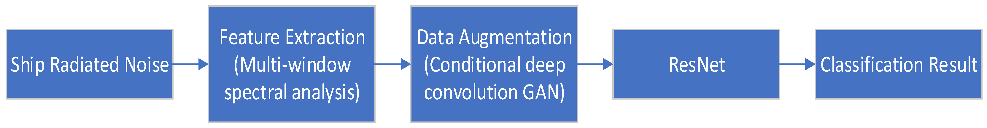
The proposed classification system is mainly composed of three parts: feature extraction, data augmentation, and classification. Figure 1 shows the structure of the classification system proposed in this paper.

In the feature extraction part, the MWSA method is used to convert the noise data into three-channel image data as the time–frequency feature of the signal, and the original sample set is constructed. In the data augmentation part, the cDCGAN model is designed to solve the problem of the insufficient number of ship-radiated noise samples. This method can effectively increase the number of samples and provide sufficient samples for the training of the classification network. To improve the training efficiency of the deep network, a classifier based on ResNet is designed to classify samples.

2.1. Multi-Window Spectral Analysis

The energy of ship-radiated noise signals is usually concentrated in a certain limited frequency band and there is a large amount of redundant information in signal waveform data. Ship-radiated noise has local stationary characteristics. T–F analysis is an effective data preprocessing method. LOFAR analysis is a common method for ship-radiated noise signal analysis, which is generally implemented based on short-time Fourier transform (STFT).

For the signal x(t), its STFT is defined as:

$$\mathrm{STFT}\left(t,f\right)=\underset{-\infty }{\overset{\infty }{{\displaystyle \int }}}\left[x\left(\tau \right)w^{*}\left(\tau -t\right)\right]e^{-j2\pi f\tau }d\tau$$

(1)

where $w\left(t\right)$ is the window function, which satisfies $||w\left(t\right)||=1$.

The discrete form of STFT is as follows:

$$\mathrm{STFT}\left(n,k\right)={\displaystyle \sum }_{m=-\infty }^{+\infty }x\left(m\right)w^{*}\left(m-n\right)e^{-j2\pi km}$$

(2)

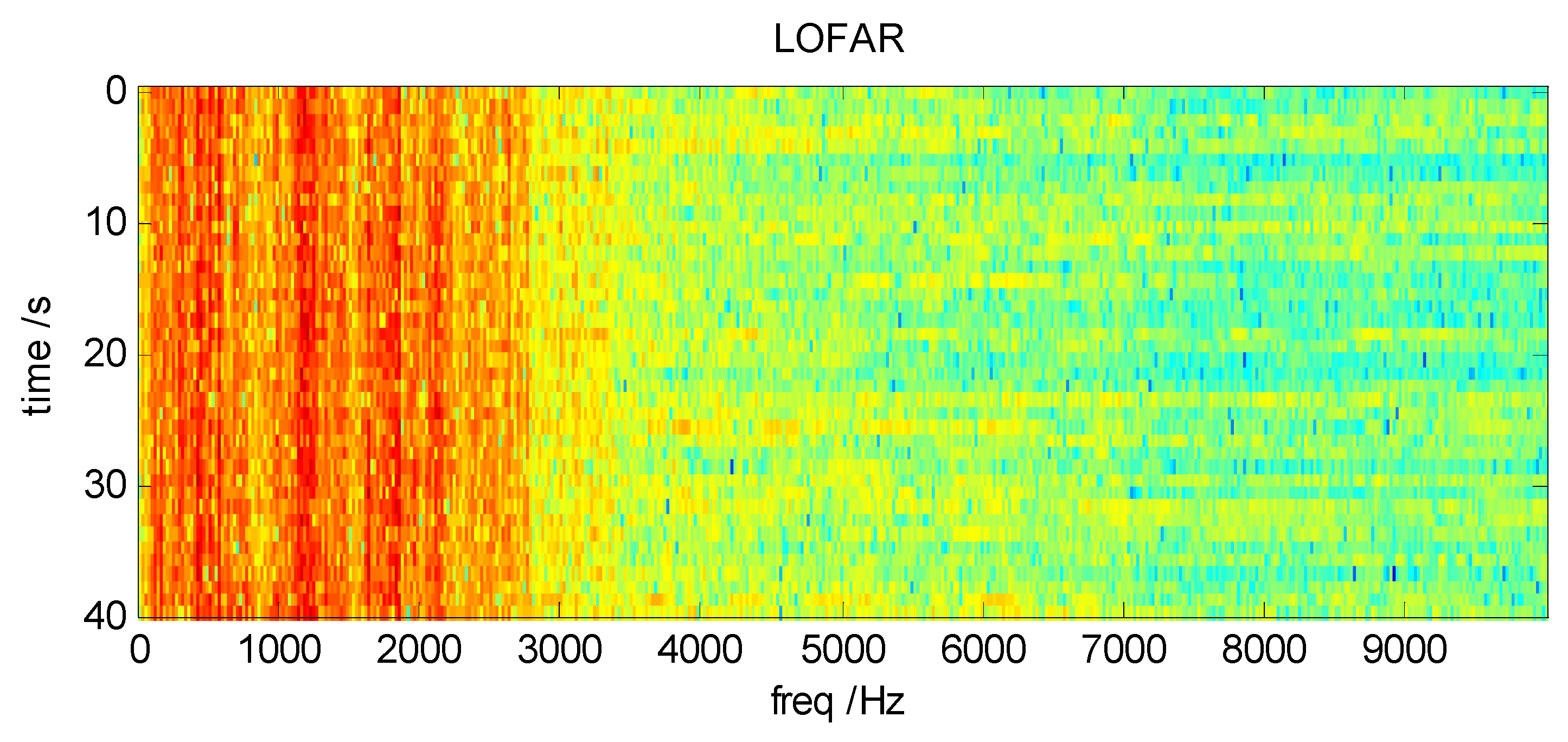
where $w\left(n\right)$ is the time window in discrete. The typical LOFAR diagram obtained by STFT method is shown in Figure 2.

Figure 2 shows the LOFAR diagram of real ship-radiated noise signals received by SONAR processed by STFT. The classification system proposed in this paper takes the LOFAR diagram as the input of feature samples. It is worth studying how to generate LOFAR diagrams with better category properties.

The time window $w\left(t\right)$ has a decisive influence on the T–F resolution of STFT analysis. In order to obtain high resolution signal energy distribution in the joint T–F domain, it is necessary to set up an energy concentration window on the T–F plane. This energy concentration is limited by the Heisenberg–Gabo uncertainty principle, which states that for a given signal, the product of its time width and bandwidth is a constant.

It is well known that short time windows provide good time resolution, but poor frequency resolution. In contrast, long time windows provide good frequency resolution, but poor time resolution.

In order to compare the time resolution and frequency resolution of various windows, the window can be described by the parameters of “time center”, “time width”, “frequency center” and “frequency width”. For $w\left(t\right)$, the definitions of these parameters are shown in

Table 1. The definitions of window parameters of $w\left(t\right)$.

Name	Expression
signal energy ($E$)	$E=||w{\left(t\right)||}^2={\displaystyle \int }{\left|w\left(t\right)\right|}^{2}dt=\frac{1}{2\pi }{\displaystyle \int }{\left|W\left(j\mathsf{\Omega }\right)\right|}^{2}d\mathsf{\Omega }$
time center ($t_0$)	$t_0=\frac{1}{E}{\displaystyle \int }t{\left|w\left(t\right)\right|}^{2}dt$
frequency center (${\mathsf{\Omega }}_0$)	${\mathsf{\Omega }}_0=\frac{1}{2\pi E}{\displaystyle \int }\mathsf{\Omega }{\left|W\left(j\mathsf{\Omega }\right)\right|}^{2}d\mathsf{\Omega }$
time width (${\Delta }_t$)	${\Delta }_t={\left(\frac{1}{E}{\displaystyle \int }{\left(t-t_0\right)}^2{\left|w\left(t\right)\right|}^{2}dt=\frac{1}{E}{\displaystyle \int }{t}^2{\left|w\left(t\right)\right|}^{2}dt-t_0^2\right)}^{\frac{1}{2}}$
frequency width (${\Delta }_{\mathsf{\Omega }}$)	${\Delta }_{\mathsf{\Omega }}={\left(\frac{1}{2\pi E}{\displaystyle \int }{\left(\mathsf{\Omega }-\mathsf{\Omega }\right)}^2{\left|W\left(j\mathsf{\Omega }\right)\right|}^{2}d\mathsf{\Omega }=\frac{1}{2\pi E}{\displaystyle \int }{\mathsf{\Omega }}^2{\left|W\left(j\mathsf{\Omega }\right)\right|}^{2}d\mathsf{\Omega }-{\mathsf{\Omega }}_0^2\right)}^{\frac{1}{2}}$

, where $W\left(j\mathsf{\Omega }\right)$ is the form in frequency domain for $w\left(t\right)$.

.

Theoretically, the Gaussian window has the smallest ${\Delta }_t{\Delta }_{\mathsf{\Omega }}=0.5$ among all the windows, which means that it has the best energy aggregation performance in the T–F plane.

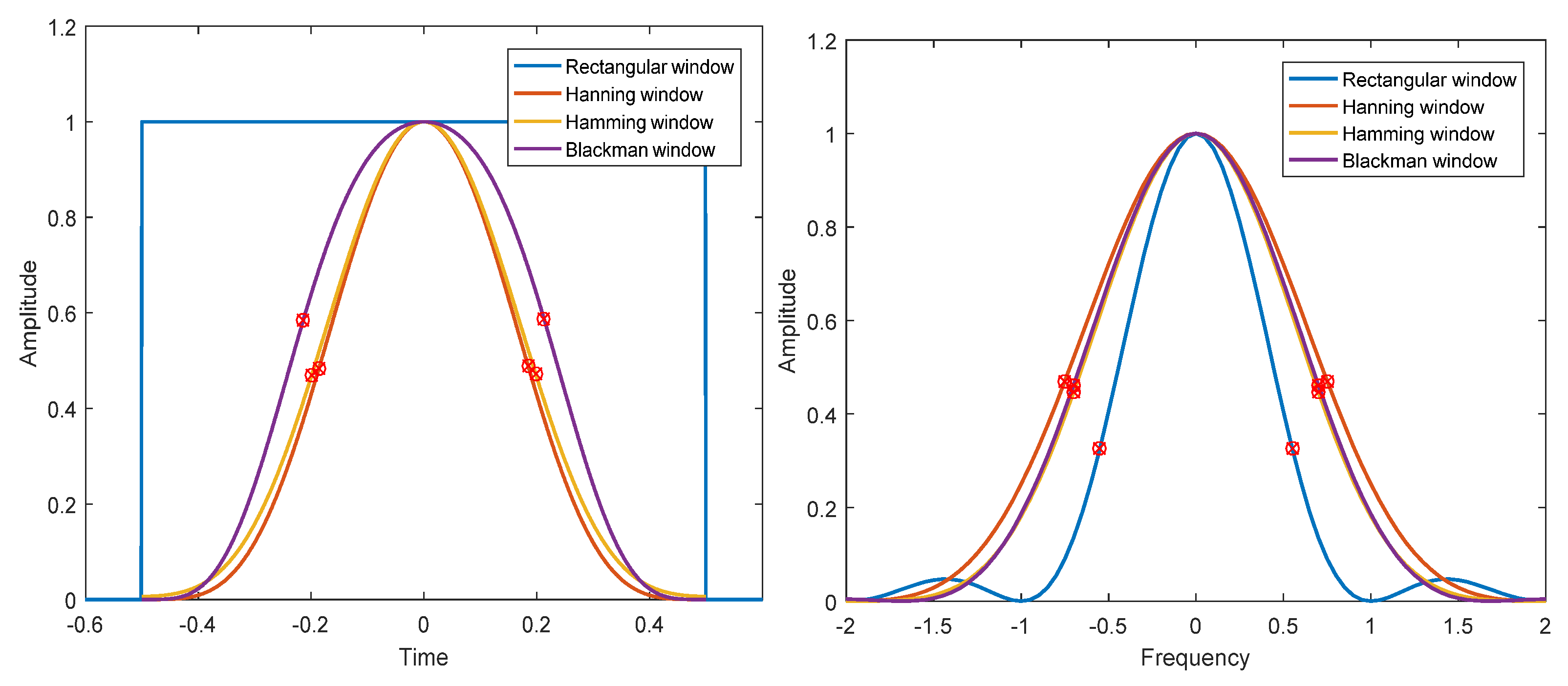
For finite length digital windows used in digital signal processing, it is not easy to calculate the corresponding ${\Delta }_t$ and ${\Delta }_{\mathsf{\Omega }}$ analytically. For the convenience of calculation, the effective width in frequency domain and time domain is redefined here. The signal time width is defined as the time from the signal center as the symmetry center to both sides until it contains 80% energy area. Similarly, the spectrum width of a signal is defined as the spectrum width from the symmetry center of the signal to both sides until it contains 80% energy area. The rectangular, Hanning, Hamming, and Blackman windows are analyzed by numerical calculation. 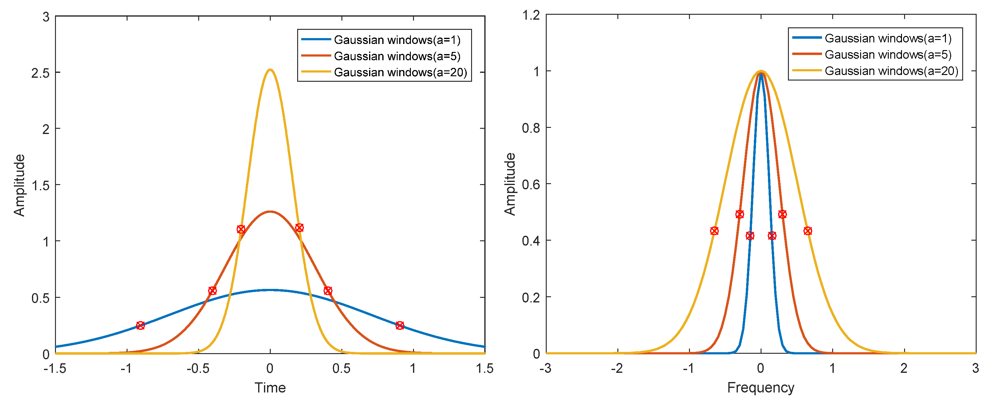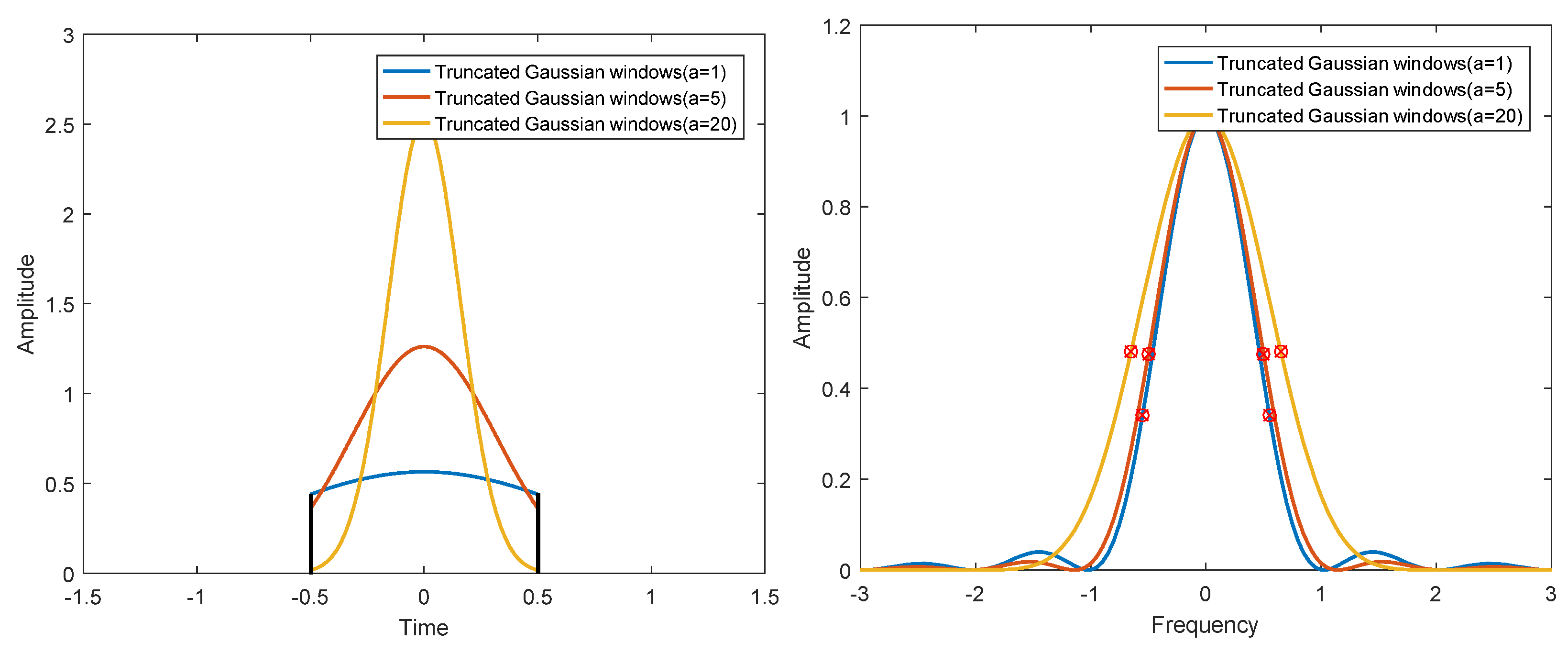The results are shown in Figure 3. Although the time bandwidth product of a Gaussian window can reach the minimum in theory, the actual Gaussian window is truncated, which has an impact on the performance of the window. The results of numerical analysis of different $\mathsf{\alpha }$-parameter Gaussian windows and truncated Gaussian windows, are shown in Figure 4 and Figure 5. The analysis results of the above windows are shown in

Table 2. Parameters of various windows (When $f_s=1 \mathrm{kHz}$ and $\mathrm{M}=1000$).

Window Function	${\mathbf{\Delta }}_{\mathit{t}}$	${\mathbf{\Delta }}_{\mathbf{\Omega }}$	${\mathbf{\Delta }}_{\mathit{t}}{\mathbf{\Delta }}_{\mathbf{\Omega }}$
Rectangular	1	1.14	1.14
Hanning	0.38	1.52	0.578
Hamming	0.404	1.26	0.549
Blackman	0.43	1.42	0.611
Gaussian ($\mathsf{\alpha }$ = 1)	$1$.794	0.32	$0$.574
Gaussian ($\mathsf{\alpha }$ = 5)	0.812	0.66	0.536
Gaussian ($\mathsf{\alpha }$ = 20)	0.406	1.28	0.519
Truncated Gaussian ($\mathsf{\alpha }$ = 1)	1	1.08	1.08
Truncated Gaussian ($\mathsf{\alpha }$ = 5)	1	1.12	1.12
Truncated Gaussian ($\mathsf{\alpha }$ = 20)	1	1.3	1.3

.

The following conclusions can be drawn from Figure 3, Figure 4 and Figure 5 and Table 2. (1) The rectangular window has the clearest time boundary, but there is serious spectrum leakage in the frequency domain, which leads to poor frequency resolution and relatively large time bandwidth product. (2) Hanning, Hamming, and Blackman windows have similar performance. The fluctuation of the spectrum is much lower than that of the rectangular window, and the time bandwidth product is close to the Gaussian window. Among the three windows, the Hamming window has the smallest time bandwidth product. (3) The energy of the Gaussian window is the most concentrated in T–F domain, and there is no fluctuation in time domain and frequency domain. However, the truncated Gaussian window has fluctuations in the spectrum, which makes the spectrum characteristics worse and widens the bandwidth. As can be seen from Table 2, the time bandwidth product of the truncated Gaussian window is almost twice as large as that of the uncut Gaussian window. Through the above analysis, we can know that the Hamming window has the best energy concentration characteristics in practical application.

To improve the feature extraction capability for signals in the T–F domain, it is effective to perform T–F transformations of signals through multiple windows. A set of windows with different time widths applied to the signal will produce a batch of spectrums with different T–F resolutions. According to the above method, the final multi-resolution time–frequency graph data can be expressed by the following formula:

$${\mathrm{MW}}_{-}\mathrm{STFT}\left(n,k,i\right)= {\alpha }_i{\left|{\displaystyle \sum }_{m=n-\frac{N}{2}}^{n+\frac{N}{2}-1}x\left(m\right)w_i\left(m-n\right)e^{-j2\pi \frac{m}{N}k}\right|}^2$$

(3)

where, $i$ represents the $i$-th window function and the $i$-th channel of the multi-resolution spectrograms. ${\alpha }_i$ represents the $i$-th weight. $w_i\left(n\right)$ represents the $i$-th window function. $N$ represents the length of the windows. In order to obtain different time–frequency resolutions and make the data obtained from multiple window functions have the same size in the time domain, this paper constructed a set of window functions based on Hamming windows, whose specific expressions are as follows:

$$w_i\left(n\right)=\{\begin{array}{c}0.54-0.46\cos \left(\frac{2\pi \left(n-\frac{N}{2}\right)}{\frac{N}{1}-1}\right),-\frac{N}{2}\le n-\frac{N}{i}<\frac{N}{2}\\ 0, \mathrm{otherwise} \end{array}$$

(4)

In order to reduce the influence brought by the length of the window function, the weight of the window function ${\alpha }_i$ is set as follows:

$${\alpha }_i=\frac{1}{H}\left({\displaystyle \sum }_{n=-\frac{N}{2}}^{\frac{N}{2}-1}{h}_0\left(n\right)/{\displaystyle \sum }_{n=-\frac{N}{2}}^{\frac{N}{2}-1}{h}_i\left(n\right)\right), i=1,2,\dots ,H$$

(5)

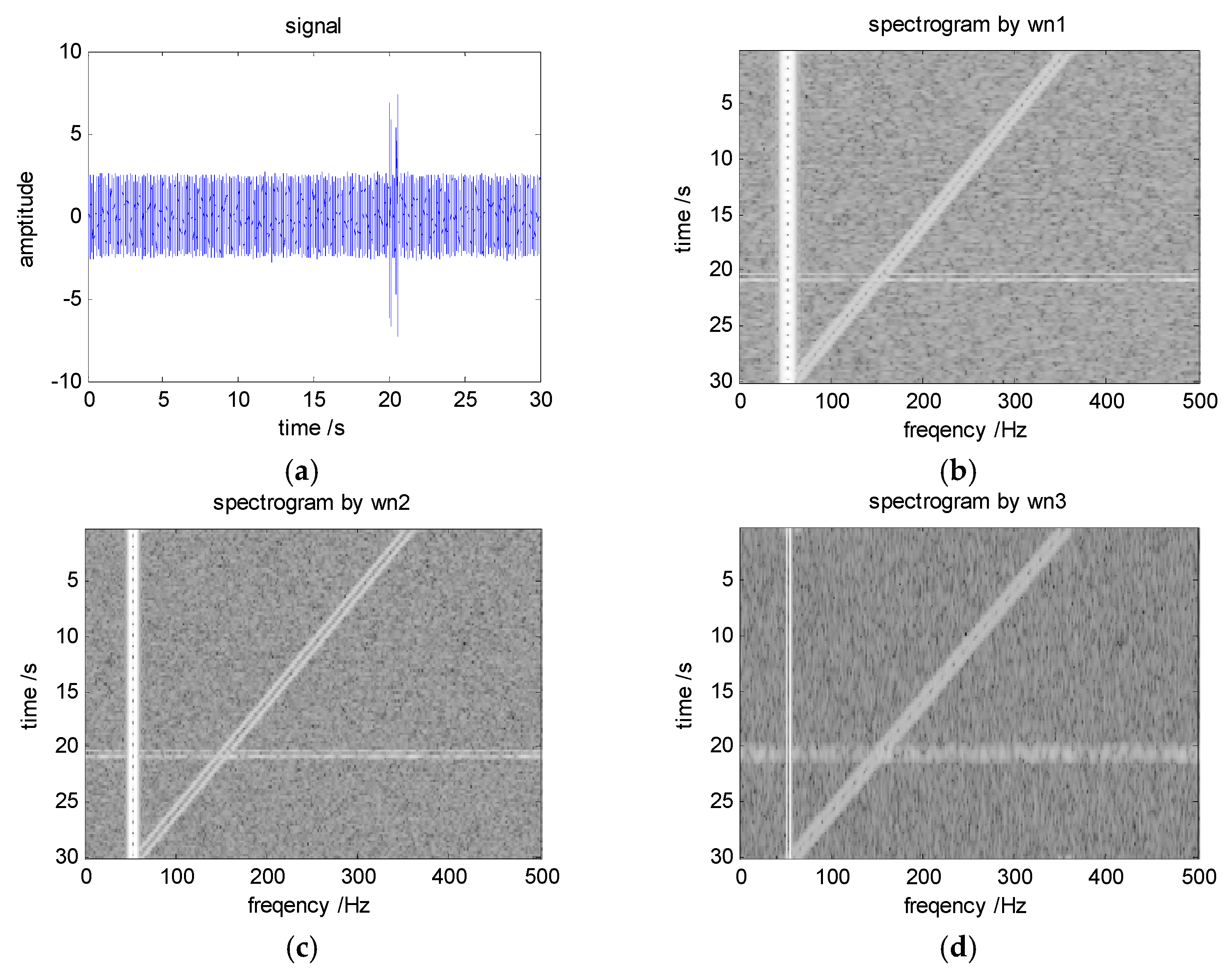
The method of MWSA is illustrated by an example of simulation signal processing. The simulation signal consists of white noise and six narrowband components. The sampling rate of the signal is 32 kHz and the duration of the signal is 30 s. The starting and ending times of the six narrow band components C1–C6 are 5 s and 25 s respectively. The parameters of narrow band components are shown in

Table 3. Parameters of simulation signal.

	Signal Type	Frequency (Hz)	Time (s)
C1	CW	50	0~30
C2	CW	55	0~30
C3	LFM	350~50	0~30
C4	LFM	355~55	0~30
C5	PULSE	/	20~20.031
C6	PULSE	/	20.125~20.156

.

These six components are three pairs of similar components used to observe the performance of different windows for different types of signals. Three windows wn1–wn3 are used to implement MWSA. The Hamming window is used in all three windows, and the corresponding time lengths are 0.125 s, 0.5 s, and 2 s. The time domain and frequency domain shapes of each window are shown in Figure 6.

As can be seen from Figure 6, wn1 has the highest time resolution and the lowest frequency resolution in all windows. C5/C6 can clearly be distinguished in the LOFAR obtained by wn1, but it is difficult to distinguish C1/C2 and C3/C4. It is difficult to distinguish the C1/C2 signals in the LOFAR obtained by wn2, but it has good resolution for C3/C4 and C5/C6. The time resolution of wn3 is low and it is difficult to distinguish the adjacent pulse. However, wn3 has the best frequency resolution.

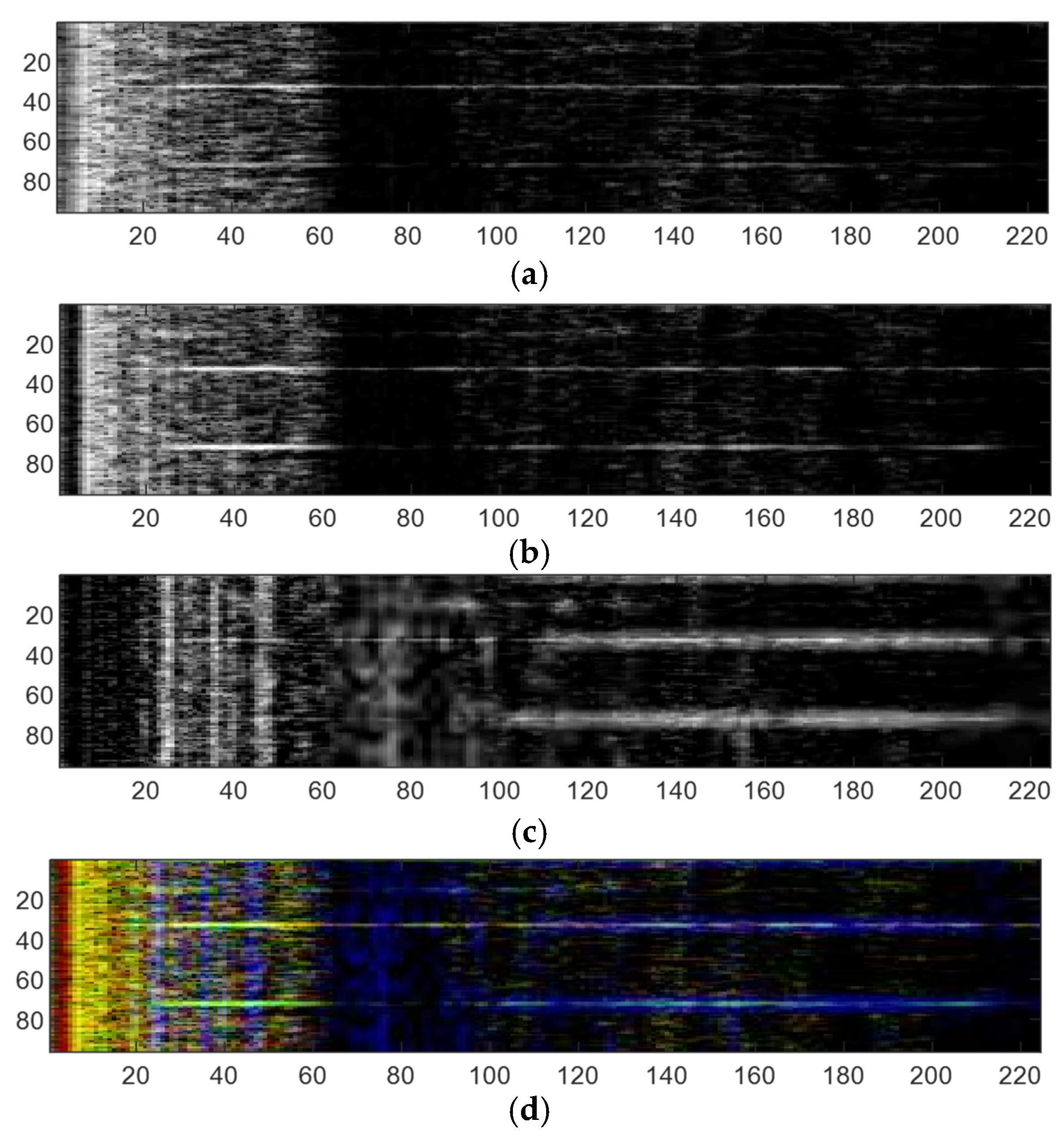
The duration of ship-radiated noise signals is not fixed. For uniformity of sample set data, the ship-radiated noise signals should be divided into several frames of fixed length through a window of suitable width. According to the MWSA method in Section 2, three window functions are set to process the sample data, and the three obtained spectrograms are stored in three channels of a color image to form the final sample. Figure 7 shows a schematic diagram of a sample construction.

2.2. Conditional Deep Convolutional GAN Model

Due to the high cost of acquiring ship-radiated noise, it is difficult to obtain sufficient samples to support the training of the classifier. In this paper, the cDCGAN model is designed based on the GAN model to expand the number of samples.

GAN consists of a generator (G) and a discriminator (D). The purpose of the generating model is to make the new generated sample as similar as possible to the training sample, while the purpose of the discriminator model is to distinguish the real sample from the generated sample as accurately as possible.

The original GAN model has two shortcomings: (1) the model does not contain label information, so the training efficiency is low; and (2) the connection structure of the generator and discriminator is simple, and the generation ability for complex samples is weak. For the problem of label information, Ref. [22] proposed the CGAN model, which introduced label information into the training process. To improve the performance of the generator and discriminator, the DCGAN model was proposed in Ref. [23], and the structure of a convolutional neural network was introduced into a GAN, which achieved good results. The cDCGAN model proposed in this paper integrates the above two models and improves them. 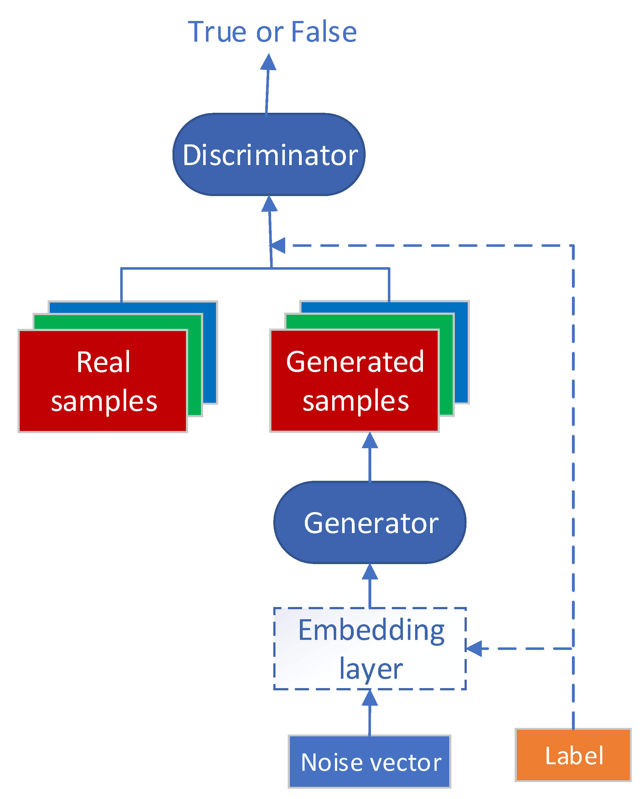Figure 8 shows the structure of the cDCGAN.

In the CGAN, the input vector is composed of a label vector and a random noise vector. The dimension extension of the generator input vector increases the processing complexity. As shown in Figure 8, the cDCGAN model is improved based on CGAN by introducing an embedding layer into the generator model. In the embedding layer, the label vector is converted to a vector of the same size as the noise vector, and then the two vectors are multiplied by elements to fuse the label information into the input noise without changing the size of the input vector. The embedding layer transforms sparse noise vectors and label vectors into dense input vectors. In the cDCGAN, the label of the sample is entered into the generator to make the generated sample category consistent with the input label. The discriminator not only determines whether the input sample is real, but also needs to judge whether the output label is correct.

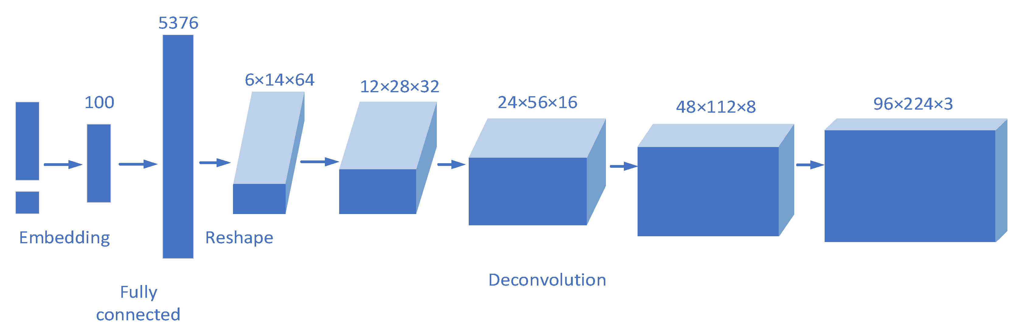
Similar to the DCGAN, the cDCGAN model improves the generator and discriminator of the GAN model; the structure of the improved generator and discriminator is shown in Figure 9 and Figure 10.

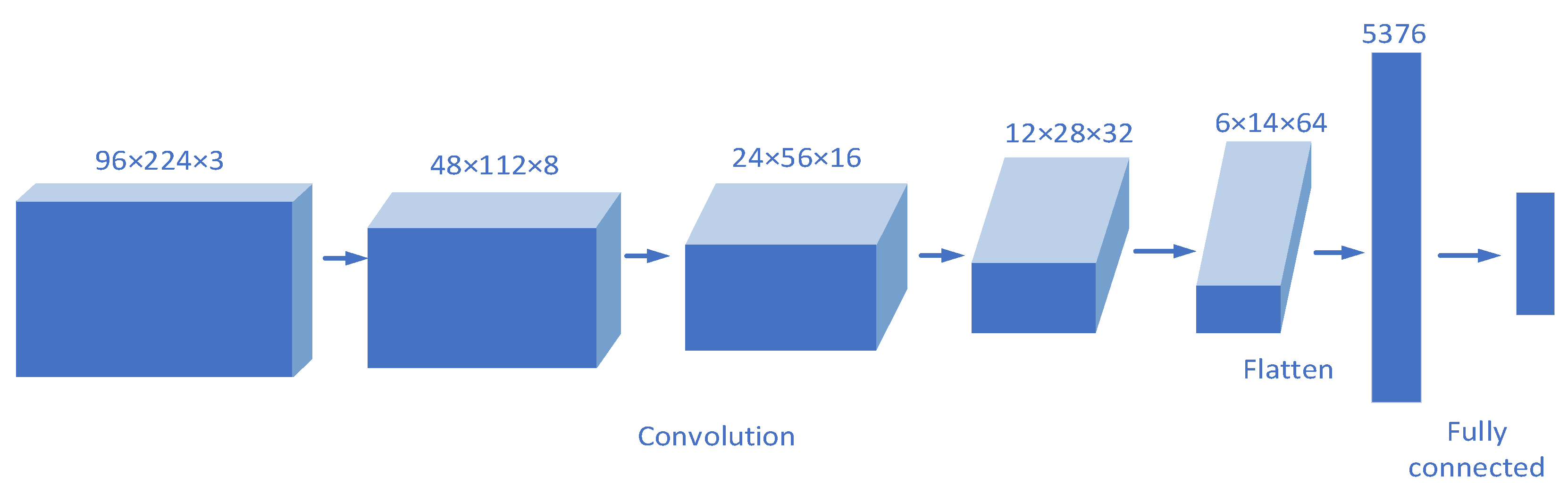
In the generator, the input vector is a fusion of random normally distributed noise and label information. First, the data size is enlarged through the fully connected layer, and then the data are reconstructed to transform the one-dimensional data into three-dimensional data of 6 × 14 × 64. Then, up-sampling is carried out step by step through the deconvolution layer and a convolution kernel with a size of 5 × 5 and a step size of 2 is used in each layer. In each layer, the size of the feature graph is doubled, and finally, after four deconvolutions, the image is gradually amplified into a 3-D image of 96 × 224 × 3.

In the discriminator, the real samples are mixed with the generated samples as the data set. The characteristics of input samples are gradually learned by down-sampling through multiple convolution layers. A convolution kernel with a size of 5 × 5 and a step size of 2 is used in each layer, and the size of the feature graph is reduced by half in each layer. After four convolution layers, the 3-D data of 6 × 14 × 64 are flattened into 1-D data and then inputted into a fully connected layer. Finally, the Sigmoid function and the SoftMax function are used to obtain the authenticity and category of the sample. The judgment of the discriminator is considered correct only when the authenticity and category of samples are both correct.

The training of the GAN is the process of game confrontation between the generator and the discriminator. The purpose of the generator is to maximize the probability of incorrect judgment of the discriminator, while the purpose of the discriminator is to maximize the probability of correct judgment. With the addition of label information, the loss function in the cDCGAN can be expressed as follows:

$$\underset{G}{\min } \underset{D}{\max }V\left(D,G\right)=E_{x~p_x\left(x\right)}\left[logD(x|c)\right]+E_{z~p_z\left(z\right)}\left[\mathit{log}\left(1-D\left(x|c\right)\right)\right]$$

(6)

where $V\left(D,G\right)$ is the value function of cDCGAN. $D$ is the output of the discriminator.$G$ is the output of the generator. $p_x\left(x\right)$ is the distribution of real samples and $p_z\left(z\right)$ is the distribution of random noises.

2.3. Classifier Based on ResNet

In deep networks, generally, the network accuracy should increase as the network depth increases. However, as the network gets deeper, a new problem arises. These layers bring a large number of parameters that need to be updated. When the gradient propagates from back to front, the gradient of the earlier layer will be very small when the network depth increases. This means that the learning of these layers stagnates, which is the vanishing gradient problem. In addition, more neural network layers mean that the parameter space is larger and parameter optimization becomes more difficult. Simply increasing the network depth will lead to higher training errors. This is not because of overfitting (the training error of the training set is still very high), but because of network degradation. ResNet designs a residual module that can effectively train deeper networks.

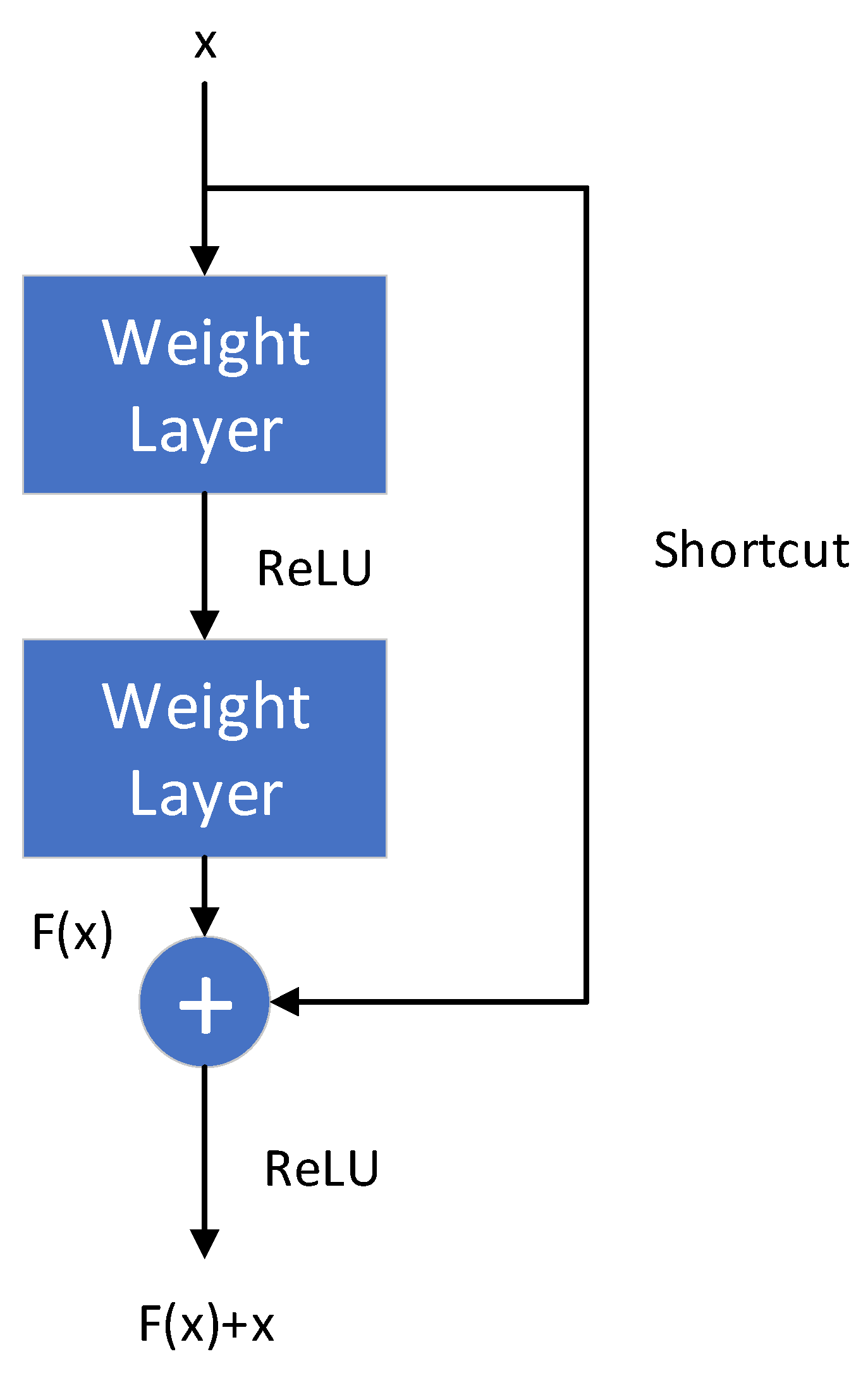
For the deep network structure, when the input is $x$, the learned features are denoted as $H\left(x\right)$, and the target learning feature can be changed to $F\left(x\right)=H\left(x\right)-x$. The reason for this is that residual learning is easier than raw feature learning. When the residual is 0, the accumulation layer only does the identity mapping and, at least, the network performance does not decline. In fact, the residual will not be 0, which will also enable the accumulation layer to learn new features based on the input features, so as to have better performance. This is similar to a “short circuit” in a circuit, so it is called a shortcut connection. The structure of residual learning is shown in Figure 11 [19].

The residual module can be expressed as:

$$x_{l+1}=f\left(h\left(x_l\right)+F\left(x_l,w_l\right)\right)$$

(7)

where $x_l$ and $x_{l+1}$ represent the input and output of the $l$-th residual unit, respectively, and each residual module generally contains a multi-layer structure.$w_l$ represents the weight from the $l$-th residual unit to the $\left(l+1\right)$-th residual unit. $F$ is the residual function, representing the learned residual, while $h\left(x_l\right)=x_l$ represents the identity mapping, and $f$ is the ReLU activation function. Based on the above formula, learning characteristics from shallow $l$ to deep $L$ can be obtained:

$$x_L=x_l+{\displaystyle \sum }_{i=l}^{L-1}F\left(x_i,w_i\right)$$

(8)

Using the chain rule, the gradient of back propagation can be roughly obtained:

$$\frac{\partial loss}{\partial x_l}=\frac{\partial loss}{\partial x_L}·\frac{\partial x_L}{\partial x_l}=\frac{\partial loss}{\partial x_L}·\left(1+\frac{\partial }{\partial x} {\displaystyle \sum }_{i=l}^{L-1}F\left(x_i,w_i\right)\right)$$

(9)

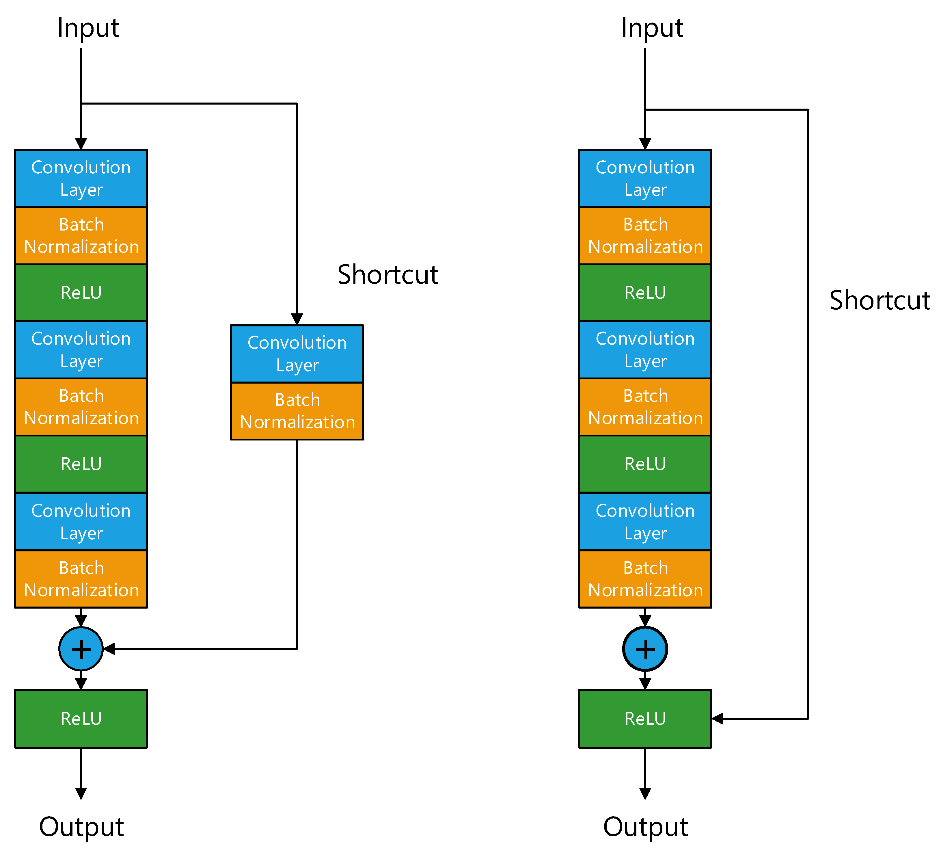
In ResNet, the residual module mainly has two forms, one is the identity block that keeps dimension unchanged, the other is the convolution block that changes dimension. Figure 12 shows the main structures of the two blocks.

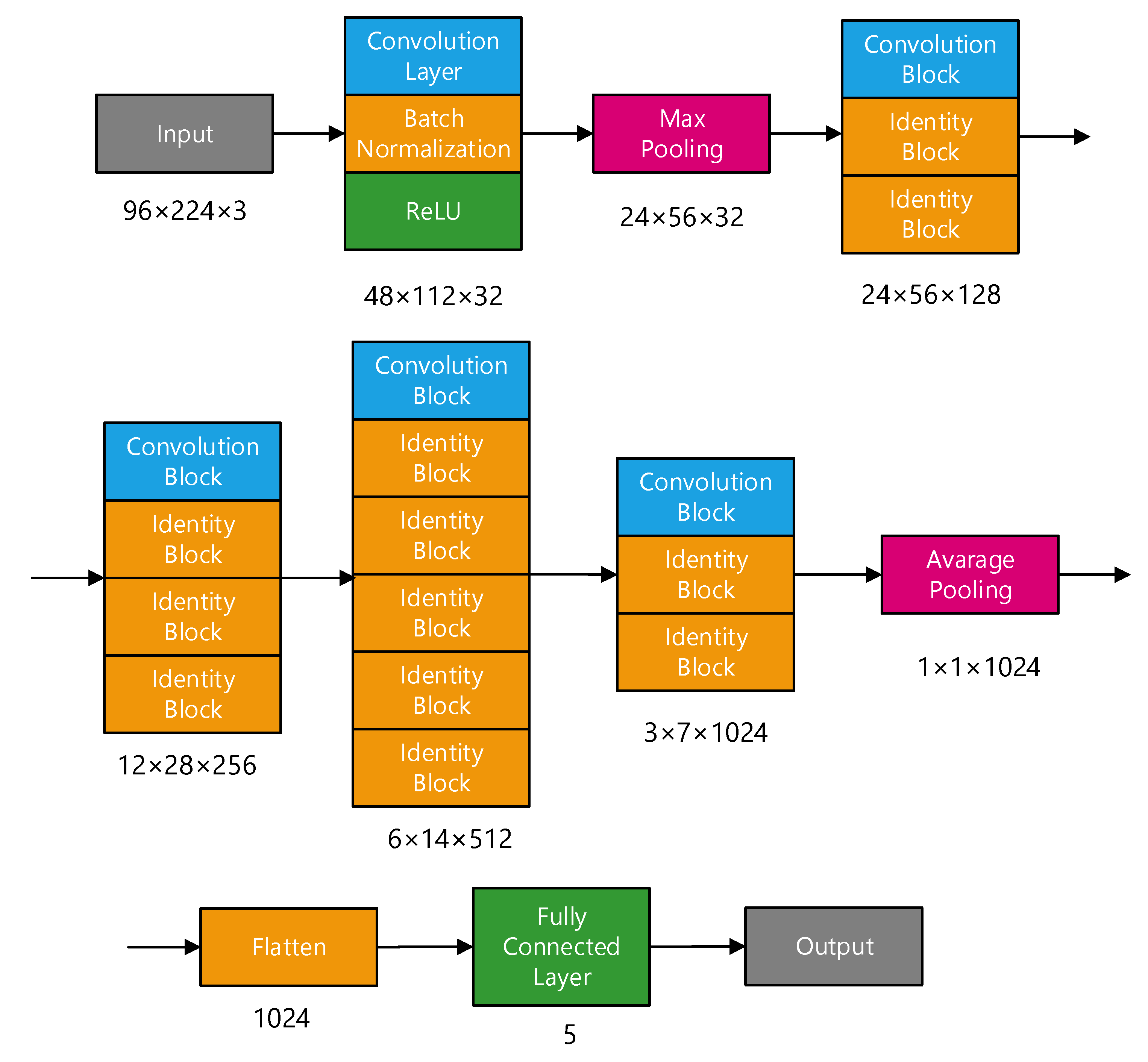
This paper designed a classification network based on ResNet; its structure is shown in Figure 13.

After feature extraction, the input sample size was 96 × 224 × 3. First, the convolution layer, batch normalization, and ReLU activation function were used to change the size to 48 × 12 × 32 by using 32 convolution kernels, and then the size was further reduced by maximum pooling. The core part of the network is composed of multiple convolution modules and identity modules. Each convolution module will halve in size and adopt a residual structure. Even if the network deepens, the problem of vanishing gradient and exploding gradient can be effectively solved. Finally, after average pooling, the size is changed to 1 × 1 × 1024. After flattening to one-dimensional data, the category of the network is output through the full connection layer. In the network, the size of the convolution kernels is 3 × 3, and the step size is 2. Meanwhile, to ensure that the total amount of learnable parameters remains unchanged, the number of convolution kernels will double every time the size of the feature graph is halved.

3. Experiment and Analysis

3.1. Experimental Database

To test the performance of the proposed UATR system, a test sample set was constructed based on the ShipsEar database [24]. The ShipsEar database is composed of 90 records representing sounds from 11 vessel types. It includes detailed information on technical aspects of the recordings and environmental and other conditions during acquisition. These recordings include many different types of vessels from the docks, including fishing boats, ocean liners, ferries of various sizes, container, roros, tugs, pilot boats, yachts, small sail boats, etc. The recordings were made with autonomous acoustic digitalHyd SR-1 recorders. This compact recorder includes a hydrophone with a nominal sensitivity of −193.5 dB re 1 V/1 uPa and a flat response in the 1 Hz–28 kHz frequency range. The amplifier chain consists of a preamplifier with a high-pass cutoff frequency of 100 Hz. The device also includes a 24-bit A/D sigma-delta converter with a sampling rate of 52,734 Hz. During data acquisition, the hydrophones were bottom-moored and attached to a submerged buoy. The distances between the recorder and the ships are less than 100 m, and some distances are less than 50 m. These distances ensure that a single hydrophone can receive ship-radiated noise with a high SNR.

Based on ship size, 11 ship types were reclassified into five categories, as shown in

Table 4. ShipsEar data classification.

Category	Type of Vessel
Class A	fishing boats, trawlers, mussel boats, tugboats and dredgers
Class B	motorboats, pilot boats and sailboats
Class C	passenger, ferries
Class D	ocean liners and ro-ro vessels
Class E	background noise recordings

.

3.2. The Construction and Augmentation of Sample Set

The samples in the ShipsEar database are single-channel audio signals with sampling rates of 52,734 Hz. In this paper, all data are divided into frames of 2 s. To obtain more samples, a 50% overlap between frames is adopted. For each data frame, the time–frequency graph is obtained by using the multi-resolution spectral analysis method. To obtain information under different time resolutions and frequency resolutions, the window lengths of the three window functions are set to 20 ms, 80 ms, and 320 ms respectively, and the frequency range to 0–3000 Hz. Subsequently, the obtained spectrograms are normalized to zero mean and unit variance and then intercepted to three standard deviations [26]. Finally, three spectrograms are stored in three channels respectively to form the final sample with a dimension of 96 × 224 × 3. Figure 14 shows the spectrogram obtained by each window and the integrated spectrogram in color.

As can be seen from Figure 14, spectrograms of different resolutions can be saved in a single-color spectrogram by MWSA processing. In this way, the spectrogram can be easily processed by the general image classification network. These colored spectrograms form an original set of samples for classification.

The cDCGAN model is trained by the original sample set, and the corresponding generator is obtained, which can generate samples of different categories based on input labels. Figure 15 shows the sample generated by the generator after different iterations.

Through the DCDGAN obtained after training, we expanded the number of samples of each category in the sample base. The number of samples before and after data augmentation is shown in

Table 5. Sample numbers before and after data augmentation.

Category	A	B	C	D	E	Total
Original number	767	624	1690	1008	465	4554
Expanded number	1500	1500	2000	1700	1000	7700

.

3.3. Experimental Results

Through the cDCGAN, various types of expanded samples are generated, and the expanded samples are combined with the original training samples to complete the data augmentation of the sample set. The enhanced training set is sent to ResNet for training, and, finally, a practical classification network can be obtained.

With the cDCGAN, the original sample set is extended. The training set was constructed by selecting samples from the extended sample set. ResNet can be trained through a training set to obtain a practical classification network.

The test set is sent to the trained ResNet network to obtain the classification results of each sample. The proposed ResNet has 50 layers. The initial learning rate is set to 0.001, the batch size is set to 128, and the activation function is ReLU. The confusion matrix corresponding to the classification results is shown in

Table 6. Confusion matrix symbol representation.

Truth	Prediction
	Class A	Class B	Class C	Class D	Class E
Class A	183	2	5	2	0
Class B	3	145	8	1	0
Class C	4	3	409	5	2
Class D	2	1	4	246	0
Class E	0	0	0	0	117

.

Furthermore, we use accuracy, recall rate, and F1 value as performance indicators to describe the performance of the classifier. For category $k, k=A,B,C,D,E$, each performance indicator is calculated as follows:

$$\mathrm{Accuracy}=\frac{n_{AA}+n_{BB}+n_{CC}+n_{DD}+n_{EE}}{N}$$

(10)

$${\mathrm{Recall}}_k=\frac{n_{kk}}{n_{kA}+n_{kB}+n_{kC}+n_{kD}+n_{kE}}$$

(11)

$${\mathrm{Precision}}_k= \frac{n_{kk}}{n_{Ak}+n_{Bk}+n_{Ck}+n_{Dk}+n_{Ek}}$$

(12)

$$\mathrm{F}1{\mathrm{score}}_k=2·\frac{{\mathrm{Precision}}_k·{\mathrm{Recall}}_k}{{\mathrm{Precision}}_k+{\mathrm{Recall}}_k}$$

(13)

where, $N$ represents the total number of test samples. $n_{ij}$ represents the number of samples of class $i$ classified as class $j$.

The accuracy of the experiment is 96.32%. The values for recall, precision, and F1 score of each category are shown in

Table 7. Experimental results.

	$\mathbf{Recall}$	$\mathbf{Precision}$	$\mathbf{F}1 \mathbf{Score}$
Class A	95.31%	95.31%	0.9531
Class B	92.36%	96.03%	0.9416
Class C	96.69%	96.01%	0.9635
Class D	97.23%	96.85%	0.9704
Class E	100.00%	98.32%	0.9915
Average	96.31%	96.50%	0.9640

.

As can be seen from Table 7, the lowest recall, precision, and F1 score are 92.36%, 95.31%, and 0.9416, respectively. The average recall, precision, and F1 score are 96.31%, 96.50%, and 0.9640, respectively. The experiment results show that the proposed UATR has good recognition ability for five categories of signals.

3.3.1. Comparison of Feature Extraction Methods

To test the effect of the multi-window spectral analysis method, single-channel LOFAR spectrum analysis, pseudo-color image analysis, and multi-window spectral analysis were used to extract features from ship data.

Single-channel LOFAR spectrum analysis is a general LOFAR spectrum analysis. For each data frame, the STFT is carried out, the window length is 80 ms, the step is 20 ms, the frequency range is 0–3000 Hz, and the size of the final sample graph is 96 × 224 × 1.

Pseudo-color image analysis is based on single-channel analysis to convert a single-channel LOFAR spectrum into a three-channel RGB image [27], using gray value as the entrance address for the color lookup table to find the corresponding value of the three channels and then produce the color image. The purpose of pseudo-color image analysis is to improve the identifiability of the graph, but it can only provide information processed by one window function.

Figure 16 shows the sample graphs of the same data frame obtained under three different pretreatment methods. GAN data augmentation was carried out on these sample sets, and classification and identification were carried out based on ResNet. The accuracy of the test sets is shown in

Table 8. Accuracy of different feature extraction methods.

Preprocessing Method	Accuracy
Single-channel spectrum analysis	92.43%
Pseudo-color image analysis	93.48%
Multi-resolution spectrum analysis	96.32%

.

As Table 8, compared with single-channel spectrograms, both pseudo-color spectrograms and multi-window spectrograms can effectively improve classification accuracy. Multi-window spectrograms can provide information under different T–F resolutions and have the best classification performance.

3.3.2. Comparison of Data Augmentation Methods

To compare the performance of the augmentation methods, six experiments were carried out based on the method of no augmentation, audio data augmentation [28], GAN augmentation, CGAN augmentation, DCGAN augmentation, and cDCGAN augmentation, respectively. The audio data augmentation method included four augmentation methods: time stretching (TS), pitch shifting (PS1), dynamic range compression (DRC), and background noise (BG).

The six experiments were trained and classified based on ResNet after multi-resolution spectrum analysis.

Table 9. Accuracy of different data augmentation methods.

Data Augmentation Method	Accuracy
No data augmentation	90.94%
Audio data augmentation [23]	92.60%
GAN data augmentation	91.35%
CGAN data augmentation	91.82%
DCGAN data augmentaion	96.14%
cDCGAN data augmentation	96.32%

shows the test results of the six data augmentation methods.

It can be seen from Table 9 that data augmentation brings gains to the classification network training. Data augmentation based on cDCGAN achieves the best results.

3.3.3. Comparison of Classification Models

We compared the performance of the ResNet model with that of the other two classifiers. One classifier is the GMM classifier based on Ref. [24], and the other is the mature classification network VGG-19. All three experiments were based on the same training and test data sets. The test results are shown in

Table 10. Accuracy of different classification models.

Classification Model	Accuracy
GMM	75.40%
VGG-19	95.79%
ResNet	96.32%

.

As can be seen from Table 10, DNN has great advantages over the traditional GMM classifier, while the ResNet model achieves the best classification results.

In addition, the training speeds of the VGG model and the ResNet model were recorded respectively, as shown in

Table 11. Training speed of different classification models.

Classification Model	Training Time
VGG-19	26 min
ResNet-50	16 min

. The methods were been simulated by MATLAB software on a workstation with an 8-core CPU (I7 9700K) and 16 GB RAM. In both cases, the loss function reached convergence and no significant changes occurred in the fifth iteration, which was taken as the cutoff time.

It can be seen from Table 11 that since ResNet can learn preload parameters through migration, the amount of training is reduced, so the training time is also significantly reduced. For each 2 s data frame, the total time of feature extraction and ResNet classification is about 16 ms.

3.3.4. Adaptability to New Samples

In the previous experiment, the training set was constructed by randomly selecting 80% of the feature samples. The training samples involved records from all 90 ships. However, in the actual work of the classifier, it is possible to encounter recorded data of new vessels, and the sample obtained from this record is never seen by the classifier. To evaluate the classification performance of the classifier on new record data, we restricted the training set construction by taking feature samples corresponding to the 80% of recorded data as training samples, and the remaining 20% of feature samples as test samples. The construction methods of the two training sets are shown in Figure 17.

It can be seen from

Table 12. Accuracy of different classification models.

Training Set Construction Method	Accuracy
Random	96.32%
According to vessel records	92.91%

that the results of the classification system have decreased, but the classification accuracy of 92.91% is acceptable. This indicates that the system has good adaptability to new samples.

4. Conclusions

In this paper, a UATR method is proposed that uses MWSA to reduce the dimension of data. Spectrograms with different T–F resolutions are calculated through three windows to synthesize a 3-channel color spectrogram as the classification feature into the classification network. Combining the advantages of CGAN and DCGAN, the cDCGAN model is designed to realize the effective augmentation of samples. The designed classification network based on ResNet gives full play to the advantages of the residual module and can realize signal classification with high efficiency and high performance. According to the experiment based on the ShipsEar database, the accuracy of the proposed method is 96.32%, which is a better classification performance than other current methods. The proposed method provides good technical support for the target classification and recognition function of a SONAR system. The performance test results of the proposed method are based on experiments with high-SNR data sets. The ship-radiated noise data obtained by actual SONAR systems usually have low SNRs and low signal-to-interference ratios (SIR). Feature extraction and data augmentation using the proposed method under a small sample set with low-SNR samples are worthy of further study.

References

1. Akyildiz, I.F.; Pompili, D.; Melodia, T. Underwater acoustic sensor networks: Research challenges. Ad Hoc Netw. 2005, 3, 257–279. [Google Scholar] [CrossRef]
2. Fang, S.; Du, S.; Luo, X.; Han, N.; Xu, X. Development of underwater acoustic target feature analysis and recognition technology. Bull. Chin. Acad. Sci. 2019, 34, 297–305. [Google Scholar]
3. Erol-Kantarci, M.; Mouftah, H.T.; Oktug, S. A survey of architectures and localization techniques for underwater acoustic sensor networks. IEEE Commun. Surv. Tutor. 2011, 13, 487–502. [Google Scholar] [CrossRef]
4. Luo, X.; Feng, Y. An underwater acoustic target recognition method based on restricted Boltzmann machine. Sensors 2020, 20, 5399. [Google Scholar] [CrossRef] [PubMed]
5. Luo, X.; Feng, Y.; Zhang, M. An underwater acoustic target recognition method based on combined feature with automatic coding and reconstruction. IEEE Access 2021, 9, 63841–63854. [Google Scholar] [CrossRef]
6. Zhang, L.; Wu, D.; Han, X.; Zhu, Z. Feature extraction of underwater target signal using mel frequency cepstrum coefficients based on acoustic vector sensor. J. Sens. 2016, 2016, 7864213. [Google Scholar] [CrossRef] [Green Version]
7. Khishe, M.; Mohammadi, H. Passive sonar target classification using multi-layer perceptron trained by salp swarm algorithm. Ocean Eng. 2019, 181, 98–108. [Google Scholar] [CrossRef]
8. Hu, G.; Wang, K.; Peng, Y.; Qiu, M.; Shi, J.; Liu, L. Deep learning methods for underwater target feature extraction and recognition. Comput. Intell. Neurosci. 2018, 2018, 1214301. [Google Scholar] [CrossRef] [PubMed]
9. Qiao, W.; Khishe, M.; Ravakhah, S. Underwater targets classification using local wavelet acoustic pattern and Multi-Layer Perceptron neural network optimized by modified Whale Optimization Algorithm. Ocean Eng. 2021, 219, 108415. [Google Scholar] [CrossRef]
10. Biernacki, C.; Celeux, G.; Govaert, G. Assessing a mixture model for clustering with the integrated completed likelihood. IEEE Trans. Pattern Anal. Mach. Intell. 2000, 22, 719–725. [Google Scholar] [CrossRef]
11. Chang, C.C.; Lin, C.J. LIBSVM: A library for support vector machines. ACM Trans. Intell. Syst. Technol. 2011, 2, 1–27. [Google Scholar] [CrossRef]
12. Khishe, M.; Mosavi, M.R. Improved whale trainer for sonar datasets classification using neural network. Appl. Acoust. 2019, 154, 176–192. [Google Scholar] [CrossRef]
13. Stewart, W.K.; Jiang, M.; Marra, M. A neural network approach to classification of sidescan sonar imagery from a midocean ridge area. IEEE J. Ocean. Eng. 1994, 19, 214–224. [Google Scholar] [CrossRef]
14. Yue, H.; Zhang, L.; Wang, D.; Wang, Y.; Lu, Z. The classification of underwater acoustic targets based on deep learning methods. Adv. Intell. Syst. Res. 2017, 134, 526–529. [Google Scholar]
15. Hershey, S.; Chaudhuri, S.; Ellis, D.P.W.; Gemmeke, J.F.; Jansen, A.; Moore, C.; Plakal, M.; Platt, D.; Saurous, R.A.; Seybold, B.; et al. CNN architectures for large-scale audio classification. In Proceedings of the 2017 IEEE International Conference on Acoustics, Speech and Signal Processing (ICASSP), New Orleans, LA, USA, 5–9 March 2017; pp. 131–135. [Google Scholar] [CrossRef] [Green Version]
16. Krizhevsky, A.; Sutskever, I.; Hinton, G.E. ImageNet classification with deep convolutional neural networks. Commun. ACM 2017, 60, 84–90. [Google Scholar] [CrossRef]
17. Simonyan, K.; Zisserman, A. Very deep convolutional networks for large-scale image recognition. arXiv 2014, arXiv:1409.1556. [Google Scholar]
18. Doan, V.S.; Huynh-The, T.; Kim, D.S. Underwater acoustic target classification based on dense convolutional neural network. IEEE Geosci. Remote Sens. Lett. 2020, 2020, 1–5. [Google Scholar] [CrossRef]
19. He, K.; Zhang, X.; Ren, S.; Sun, J. Identity Mappings in Deep Residual Networks. In Proceedings of the European Conference on Computer Vision, Amsterdam, The Netherlands, 11–14 October 2016; Springer: Cham, Swizterland, 2016; pp. 630–645. [Google Scholar]
20. Perez, L.; Wang, J. The effectiveness of data augmentation in image classification using deep learning. arXiv 2017, arXiv:1712.04621. [Google Scholar]
21. Goodfellow, I.; Pouget-Abadie, J.; Mirza, M.; Xu, B.; Warde-Farley, D.; Ozair, S.; Courville, A.; Bengio, Y. Generative adversarial nets. In Advances in Neural Information Processing Systems; ACM Digital Library: New York, NY, USA, 2014; Volume 27. [Google Scholar]
22. Mirza, M.; Osindero, S. Conditional generative adversarial nets. arXiv 2014, arXiv:1411.1784. [Google Scholar]
23. Radford, A.; Metz, L.; Chintala, S. Unsupervised representation learning with deep convolutional generative adversarial networks. arXiv 2015, arXiv:1511.06434. [Google Scholar]
24. Santos-Domínguez, D.; Torres-Guijarro, S.; Cardenal-López, A.; Pena-Jimenez, A. ShipsEar: An underwater vessel noise database. Appl. Acoust. 2016, 113, 64–69. [Google Scholar] [CrossRef]
25. Hong, F.; Liu, C.; Guo, L.; Chen, F.; Feng, H. Underwater acoustic target recognition with a residual network and the optimized feature extraction method. Appl. Sci. 2021, 11, 1442. [Google Scholar] [CrossRef]
26. Donahue, C.; McAuley, J.; Puckette, M. Adversarial audio synthesis. arXiv 2018, arXiv:1802.04208. [Google Scholar]
27. Sharan, R.V.; Moir, T.J. Pseudo-color cochleagram image feature and sequential feature selection for robust acoustic event recognition. Appl. Acoust. 2018, 140, 198–204. [Google Scholar] [CrossRef]
28. Salamon, J.; Bello, J.P. Deep convolutional neural networks and data augmentation for environmental sound classification. IEEE Signal Process. Lett. 2017, 24, 279–283. [Google Scholar] [CrossRef]
Figure 1. The structure of the proposed classification system.
Jmse 09 01246 g001
Figure 2. LOFAR of ship-radiated noise signal.
Jmse 09 01246 g002
Figure 3. Time domain (left) and frequency domain (right) of different windows.
Jmse 09 01246 g003
Figure 4. Time domain (left) and frequency domain (right) of different Gaussian windows.
Jmse 09 01246 g004
Figure 5. Time domain (left) and frequency domain (right) of different truncated Gaussian windows.
Jmse 09 01246 g005
Figure 6. Signal waveform (a) and spectrograms of the signal (b) by wn1, (c) by wn2, and (d) by wn3.
Jmse 09 01246 g006
Figure 7. Sample storage method for multi-resolution spectrum analysis.
Jmse 09 01246 g007
Figure 8. Structure of the cDCGAN.
Jmse 09 01246 g008
Figure 9. Generator structure.
Jmse 09 01246 g009
Figure 10. Discriminator structure.
Jmse 09 01246 g010
Figure 11. Residual module structure.
Jmse 09 01246 g011
Figure 12. Convolution block and identity block.
Jmse 09 01246 g012
Figure 13. ResNet structure.
Jmse 09 01246 g013
Figure 14. (a) Spectrogram by 20 ms window, (b) spectrogram by 80 ms window, (c) spectrogram by 320 ms window, (d) spectrogram by MWSA.
Jmse 09 01246 g014
Figure 15. Generated samples under different iterations.
Jmse 09 01246 g015
Figure 16. Samples of different preprocessing methods: (a) single-channel LOFAR spectrum (96 × 224 × 1), (b) pseudo-color LOFAR spectrum (96 × 224 × 3), (c) multi-resolution time–frequency spectrum (96 × 224 × 3).
Jmse 09 01246 g016aJmse 09 01246 g016b
Figure 17. Two construction methods for the training set and test set: (left) random, (right) according to vessel records.
Jmse 09 01246 g017