Abstract
Dramatic environmental changes have been recently reported in the Yellow Sea (YS), the South Sea of Korea (SS), and the East/Japan Sea (EJS), but little information on the regional primary productions is currently available. Using the 13C-15N tracer method, we measured primary productions in the YS, the SS, and the EJS for the first time in 2018 to understand the current status of marine ecosystems in the three distinct seas. The mean daily primary productions during the observation period ranged from 25.8 to 607.5 mg C m−2 d−1 in the YS, 68.5 to 487.3 mg C m−2 d−1 in the SS, and 106.4 to 490.5 mg C m−2 d−1 in the EJS, respectively. In comparison with previous studies, significantly lower (t-test, p < 0.05) spring and summer productions and consequently lower annual primary productions were observed in this study. Based on PCA analysis, we found that small-sized (pico- and nano-) phytoplankton had strongly negative effects on the primary productions. Their ecological roles should be further investigated in the YS, the SS, and the EJS under warming ocean conditions within small phytoplankton-dominated ecosystems.
1. Introduction
Marine phytoplankton as primary producers play an important role as the base of the ecological pyramid in the ocean and are responsible for nearly a half of global primary production [1,2]. The primary production of phytoplankton is widely used as an important indicator to predict annual fishery yield in various oceanic regions [3,4,5], because it is one of key factors in determining amount of food source for upper-trophic-level consumers [6,7]. Lee et al. [8,9] also reported that an algorithm for estimation of the habitat suitability index for the mackerels and squids around the Korean peninsula was largely improved by including a primary production term. The physiological conditions and community structures of phytoplankton are closely related to physical and chemical factors (e.g., light regime, nutrients, and temperature) [10,11,12], which induce greatly different phytoplankton productions in various marine ecosystems [3,13,14]. Thus, the primary production measurements can provide fundamental backgrounds for better understanding marine ecosystems with different environmental conditions and detecting current potential ecosystem changes.
The Yellow Sea (hereafter YS), the South Sea of Korea (SS), and the East/Japan Sea (EJS), belonging to the East Asian marginal seas, have experienced 2–4 times faster increase (0.7–1.2 °C) in seawater temperature than that in global mean water temperature (0.4 °C) for 20 years (1983–2006) [15]. Moreover, some notable changes in physicochemical conditions were reported, such as increasing limitation of nutrients in the YS and rapid ocean acidification and shoaling of the mixed layer depth in the EJS [16,17,18,19]. These recent environmental changes could result in alterations in biological characteristics, including community structure and bloom pattern of phytoplankton and subsequently higher-trophic-level organisms [12,20,21,22]. Indeed, biological responses related to phytoplankton were observed in the YS [16,18,23,24] and the EJS [12,22,25,26]. For the YS, a remarkable decrease in chlorophyll-a (chl-a) concentration and phytoplankton diversity and abundance was observed between the periods 1983–1986 and 1996–1998, which affected the primary production [16]. The phytoplankton community assemblage was also dramatically changed in the YS, especially in the spring [18,23]. For the EJS, the patterns of timing, magnitude, and duration of the spring phytoplankton bloom were significantly different between 1998–2001 and 2008–2011 [25]. Joo et al. [26] found dramatic decreasing trends (1.3% each year) in annual primary productivities in various regions in the EJS for 1 decade (2003–2012) based on the satellite-based data. Nevertheless, we still have a lack of information on regional primary productions of phytoplankton for understanding the current status of the marine ecosystems in the YS, the SS, and the EJS.
In this study, one of our main objectives is to compare the seasonal and regional primary productions measured simultaneously in the YS, the SS, and the EJS for the first time in 2018 with those reported in previous studies in each region. The other one is to determine major controlling factors in the low primary production in the YS, the SS, and the EJS in 2018.
2. Materials and Methods
2.1. Water Sampling Collection
Seasonal cruise surveys were conducted onboard the R/V Tamgu 8 for the YS and the SS and R/V Tamgu 3 for the EJS from February to October 2018 (Figure 1). The data collected from the February, April, August, and October 2018 cruises were designated to represent winter, spring, summer, and autumn, respectively. At mid-morning, 9–10 different stations were determined in the YS and the EJS whereas 6–7 sampling stations were determined for the SS among the monitoring stations (Figure 1) managed by the National Institute of Fisheries Science (NIFS) in Korea (Table 1).
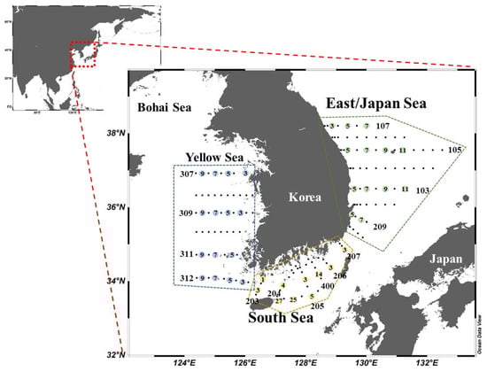
Figure 1.
Locations of sampling regions in 2018. The station numbers are in consecutive order from coast to open sea as marked in each station line.

Table 1.
Description of sampling sites in the YS, the SS, and the EJS for each cruise period, in 2018. (o) means investigation was conducted, while (-) means investigation was not conducted.
The bottom depths at our sampling stations in the YS and the SS had relatively narrow range, whereas the EJS had a wide range of bottom depths (48–2340 m) in this study (Table 1). The six water depths were determined at each station by converting Secchi disc depth to 6 corresponding light depths (100, 50, 30, 12, 5, and 1% of surface photosynthetic active radiation; (PAR)). Then, each water sample was collected from 6 different depths using Niskin bottles (8 L) equipped with a conductivity, temperature, and depth (CTD)-rosette. The water temperature and salinity were obtained from SBE9/11 CTD (Sea-Bird Electronics, Bellevue, WA, USA). The mixed-layer depth (MLD) was defined as the depth at which the density is increased by 0.125 density units from the sea surface density [27,28]. Water samples for dissolved inorganic nutrients (NH4, NO2 + NO3, PO4, and SiO2) and chl-a (total and size-fractionated) concentrations were collected at three light depths (100, 30, and 1% of PAR). Water samples for measuring the particle organic carbon (POC) and particle organic nitrogen (PON) concentrations and total carbon uptake rates (primary production) of phytoplankton were collected at six light depths (100, 50, 30, 12, 5, and 1% of PAR). The euphotic zone is defined as the depth from 100 to 1% of PAR.
2.2. Inorganic Nutrients Concentrations
To measure concentrations of dissolved inorganic nutrients (NH4, NO2 + NO3, PO4, and SiO2), 0.1 L water samples were filtered onto Whatman GF/F filters (ø = 47 mm) at a vacuum pressure lower than 150 mmHg. Filtered water samples were immediately frozen at −20 °C for further analysis in our laboratory. An auto-analyzer (Quattro, Seal Analytical, Norderstedt, Germany) in the NIFS was used for the analysis of dissolved inorganic nutrients according to the manufacturer’s instruction.
2.3. Chl-a Concentration
The primary method and calculation for determining the chl-a concentrations were conducted according to Parsons et al. [29]. Water samples (0.1–0.4 L) for total chl-a concentration were filtered through Whatman GF/F filters (ø = 25 mm), and samples (0.3–1 L) for three different size-fractionated chl-a concentrations were passed sequentially through 20 μm and 2 μm membrane filters (ø = 47 mm) and GF/F filters (ø = 47 mm) at low vacuum pressure. The filtered samples were then placed in a 15 mL conical tube, immediately stored in −20 °C freezer until the analysis. In the laboratory, the frozen filters were extracted with 90% acetone at 4 ˚C for 20–24 h, and chl-a concentrations were then measured using a fluorometer (Turner Designs, 10-AU, San Jose, CA, USA) calibrated based on commercially available reference material for chl-a.
2.4. Measurements of Phyoplankton Carbon and Nitrogen Uptake Rate
The 13C-15N dual stable isotope tracer technique was used for simultaneously measuring the carbon and nitrogen uptake rates of the phytoplankton as described by Dugdale and Goering [30] and Hama et al. [31]. In brief, water samples from each light depth (100%, 50%, 30%, 12%, 5%, and 1% of PAR) were immediately transferred to acid-rinsed polycarbonate incubation bottles (1 L) covered with neutral density screens (Lee Filters) [32] after passing through 333 µm sieves to eliminate the large zooplankton. The incubation bottles filled with seawater at each light depth were inoculated with the labeled carbon (NaH13CO3) and nitrate (K15NO3) or ammonium (15NH4Cl), which correspond to 10–15% of the concentrations in the ambient water [30,31]. Then, the tracer-injected bottles were incubated in a large polycarbonate incubator at a constant temperature maintained by continuously circulating sea surface water under natural surface light for 4–5 h. The incubated water samples (0.1–0.4 L) were filtered onto Whatman GF/F filters (ø = 25 mm) precombusted at 450 °C, and the filters were then kept in a freezer (−20 ˚C) until mass spectrometer analysis. At the laboratory of Pusan National University, the filters were fumed with a strong hydro acid in a desiccator to remove the carbonate overnight and dried with a freeze drier for 2 h. Then, POC and PON concentrations and atom % of 13C were analyzed by Finnigan Delta+XL mass spectrometer at the stable isotope laboratory of the University of Alaska (Fairbanks, AK, USA). The carbon uptake rates of the phytoplankton were estimated as described by Dugdale and Goering [30] and Hama et al. [31]. The final values of the carbon uptake rates of phytoplankton were then calculated by subtracting the carbon uptake rates of dark bottles to eliminate the heterotrophic bacterial production [33,34,35]. The daily primary productions of phytoplankton were calculated from the hourly primary productions observed in this study and 10-h photoperiod per day reported previously in the YS and EJS [22,24].
2.5. Statistical Analysis
The statistical analyses for Pearson’s correlation, t-test, and one-way analysis of variance (one-way ANOVA) were performed using SPSS (version 12.0, SPSS Inc., Chicago, IL, USA). In the one-way ANOVA, a test to certify the homoscedasticity of variables was conducted by using Levene’s test. To compare pairwise differences for the variables, Scheffe’s (homogeneity) and Dunnett’s (heteroscedasticity) post hoc tests were used, based on homogeneity of variances.
Principal component analysis (PCA) with the Varimax method with Kaiser normalization using the XLSTAT software (Addinsoft, Boston, MA, USA) was used to identify relatively significant factors affecting the total carbon uptake rates of phytoplankton in each sea during our observation time. Fourteen variables for PCA included physical (water temperature and salinity and euphotic and mixed-layer depths), chemical (NH4, NO2+NO3, PO4, and SiO2 concentrations), and biological (total and size-fractionated chl-a and POC concentration) factors and carbon uptake rates of phytoplankton.
3. Results
3.1. Physicochemical Environmental Conditions
Seasonal vertical profiles of the mean temperatures and salinities at each light depth in the YS, the SS, and the EJS are presented in Figure 2. Seasonal water temperatures and salinities in the YS, the SS, and the EJS were evenly distributed within the euphotic zone except in August. The mean temperatures within the euphotic zone in the YS, the SS, and the EJS were lowest in February, with means of 5.9 (S.D. = ± 2.3), 13.6 (± 1.3), and 9.9 (± 1.7) ˚C, respectively, and gradually increased to their highest in August, with means of 23.2 (± 1.4), 23.8 (± 1.6), and 20.9 (± 2.9) ˚C, respectively (Figure 2). The average water temperature in the YS was significantly lower than those in the SS and EJS during February and April (one-way ANOVA, p < 0.05). The highest mean salinities in the YS and EJS were observed in April (32.8 ± 0.8 and 34.4 ± 0.1 psu), whereas salinity in the SS was highest in February at 34.6 ± 0.0 psu (Figure 2). Overall, lower salinities were found in the YS than in the SS and the EJS throughout the observation period.
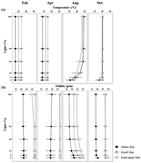
Figure 2.
Vertical profiles of mean temperatures (a) and salinities (b) at six light depths (100, 50, 30, 12, 5, and 1%) in the YS, the SS, and the EJS, 2018.
The mean euphotic depths in the YS, the SS, and the EJS were deepest in August at 37.6 ± 15.6, 49.8 ± 11.3, and 54.4 ± 10.7 m, respectively (Figure 3). In particular, the euphotic depth in the EJS in February (51.0 ± 5.8 m) was significantly deeper (one-way ANOVA, p < 0.01) than those in the YS (12.8 ± 6.2 m) and the SS (28.1 ± 4.7 m). The deepest MLDs in the YS, the SS, and the EJS were observed in February, with means of 68.7 ± 15.7, 59.0 ± 40.5, and 80.6 ± 57.4 m, respectively (Figure 3). The MLDs in the YS, the SS, and the EJS became continuously shallow until August at 12.0 ± 14.2, 13.7 ± 6.6, and 13.2 ± 6.2 m, respectively, and then deepened in October to 26.3 ± 13.7, 30.2 ± 16.1, and 37.9 ± 14.2 m, respectively. In all regions, the differences between the MLDs and euphotic depths were greatest in February, decreased toward April, and then reversed in August when MLDs were significantly shallower than the euphotic depths (t-test, p < 0.01) (Figure 3). These results indicate that the euphotic zone was vertically well-mixed in all study regions during February and April, whereas strong stratifications were developed in the euphotic water columns during August.
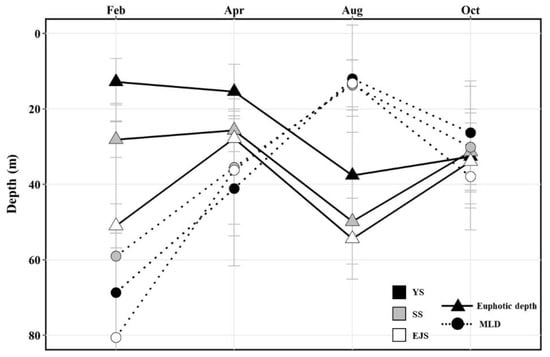
Figure 3.
Variation in the mean euphotic and mixed-layer depths in the YS, the SS, and the EJS, 2018.
Major dissolved inorganic nutrient concentrations at each light depth (100%, 30%, and 1%) in the YS, the SS, and the EJS for each cruise are summarized in Table 2. The ranges of NO2+NO3, PO4, and SiO2 concentrations during the study period were 0.5–9.9, <0.1–0.6, and 2.4–10.0 μM in the YS; 0.9–8.1, 0.1–0.4, and 5.1–11.3 μM in the SS; and 0.2–8.7, 0.1–0.5, and 2.4–11.0 μM in the EJS, respectively. Ranges of nutrient concentrations except for NH4 varied significantly in all regions during the study period, being generally high in February and low in other seasons except NO2+NO3 concentrations in the YS in April. The nutrient concentrations, except for NH4 at 1% light depths in the YS and the EJS, were higher (one-way ANOVA, p < 0.01) than those at 100% and 30% light depths during August and October, whereas vertical differences in the SS were only detected in August. NH4 concentrations ranged from 0.5 to 1.2 μM in the YS, 0.1 to 0.6 μM in the SS, and 0.4 to 0.9 μM in the EJS, respectively, during the observation period. Unlike other nutrients, NH4 concentrations had no distinct seasonal and vertical characteristics in all study regions.
Table 2.
The dissolved inorganic nutrient concentrations averaged from each light depth (100, 30, and 1%) in the YS, the SS, and the EJS, 2018.
3.2. Concentrations and Size-Fractionated Compositions of chl-a
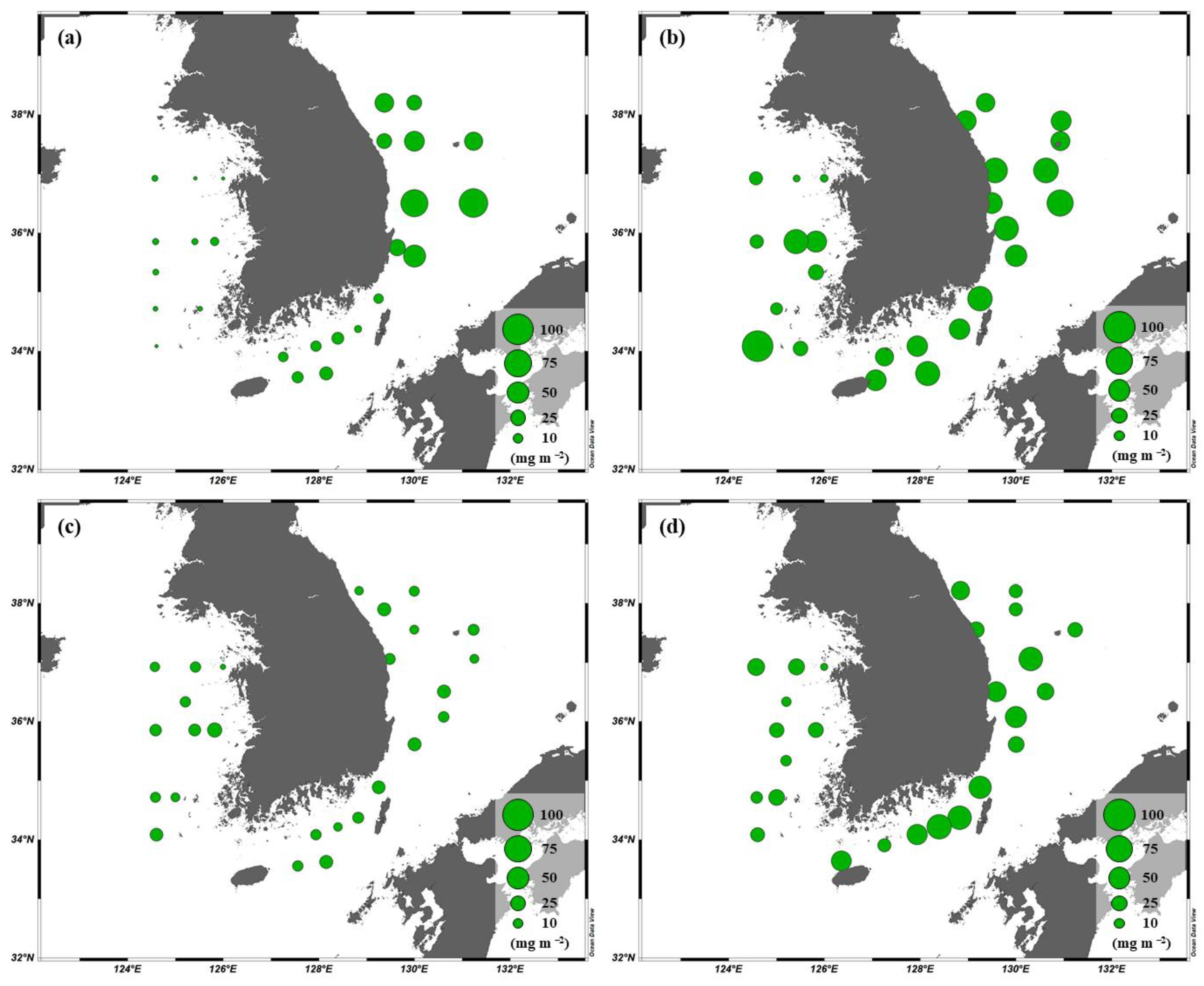
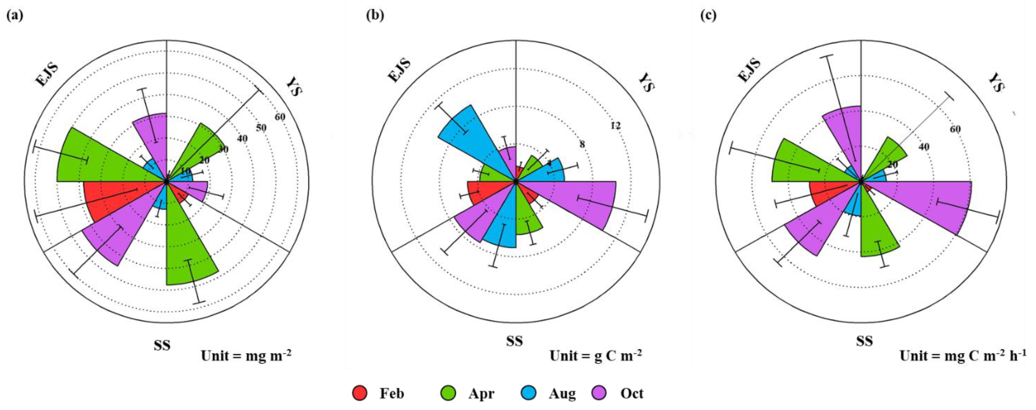
The ranges of the total chl-a concentrations integrated throughout the euphotic water column in the YS, the SS, and the EJS were 1.3–96.6, 5.6–60.7, and 8.0–92.9 mg m−2, respectively, during our observation period (Figure 4). The highest chl-a concentration in the YS was detected in April (mean ± S.D. = 31.1 ± 28.6 mg m−2), followed by October (18.8 ± 8.0 mg m−2), August (12.1 ± 5.0 mg m−2), and February (3.3 ± 1.8 mg m−2). The chl-a concentrations in the SS between April (47.6 ± 10.1 mg m−2) and October (44.9 ± 15.3 mg m−2) were similar, and the concentrations during these periods were higher (One-way ANOVA, p < 0.05) than those in February (11.7 ± 3.9 mg m−2) and August (12.8 ± 3.9 mg m−2). In the EJS, the highest chl-a concentration was observed in April (50.1 ± 12.5 mg m−2), and the second-highest concentration was observed in February (38.0 ± 23.9 mg m−2). The chl-a concentration was lowest in August (12.6 ± 4.6 mg m−2).
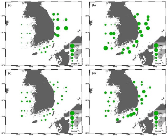
Figure 4.
Spatial distributions of the chl-a concentrations integrated within the euphotic depth from 100 to 1% light depth in the YS, the SS, and the EJS during Feb. (a), Apr. (b), Aug. (c), and Oct. (d).
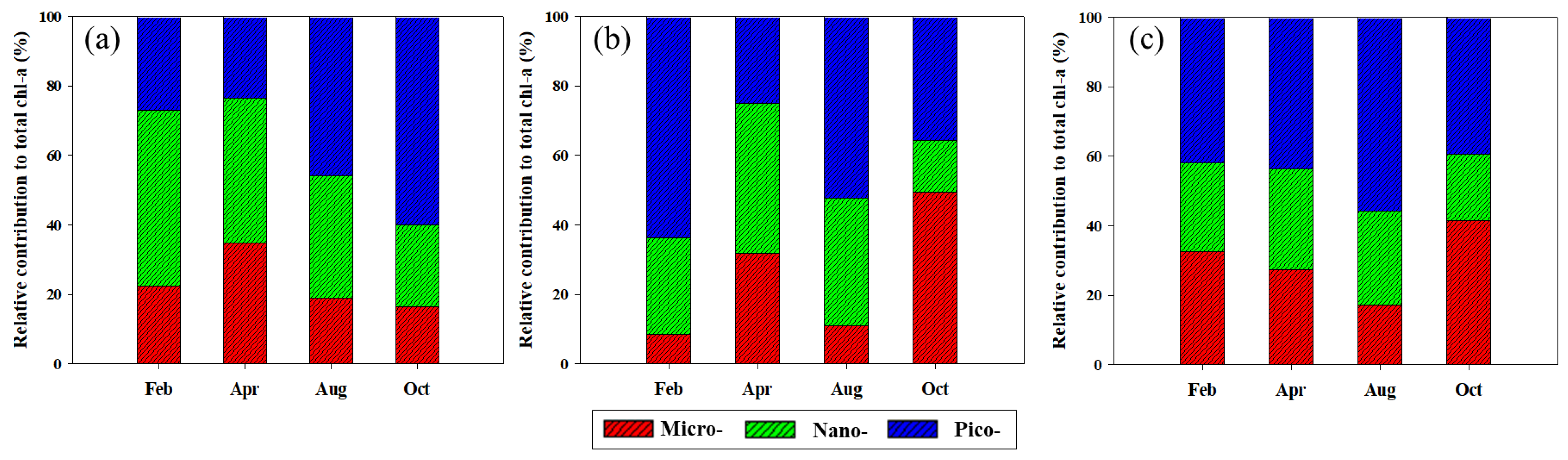
Based on the size-fractionated chl-a concentrations, the compositions of micro- (>20 μm), nano- (2–20 μm), and pico-sized (0.7–2 μm) phytoplankton in the YS, the SS, and the EJS are shown in Figure 5a–c. Overall, the fraction of nano- and pico-sized phytoplankton was dominant in the YS (> 65%), the EJS (> 58%), and the SS (> 65%) during the study period except for October. In detail, the compositions of the nano- and pico-sized phytoplankton in the YS were 50.7 ± 6.1 and 27.0 ± 12.2% in February, 41.6 ± 14.1 and 23.6 ± 10.9% in April, 35.1 ± 7.6 and 45.9 ± 14.7% in August, and 23.4 ± 6.1 and 60.1 ± 21.4% in October, respectively. The compositions of micro-sized phytoplankton in the YS remained low (approximately 19%) during the study period except for April (34.8 ± 22.8%). The contributions of the nano- and pico-sized phytoplankton in the SS during February, April, August, and October were 27.7 ± 4.4 and 63.8 ± 3.5%, 43.3 ± 19.5 and 24.9 ± 13.2%, 36.7 ± 11.5 and 52.4 ± 8.8%, and 15.0 ± 2.6 and 35.6 ± 17.5%, respectively. The highest contribution of micro-sized phytoplankton in the SS was observed in October (49.4 ± 19.5%), followed by April (31.7 ± 30.5%), August (10.9 ± 3.8%), and February (8.4 ± 2.1%). The fractions of nano- and pico-sized phytoplankton in the total chl-a concentrations in the EJS in each season were 25.4 ± 9.2 and 42.0 ± 16.6% (February), 28.8 ± 8.3 and 43.8 ± 12.7% (April), 26.9 ± 13.3 and 55.9 ± 16.6% (August), and 19.0 ± 5.5 and 39.5 ± 18.0% (October), respectively. The fraction of micro-sized phytoplankton in the EJS was gradually decreased from February (32.7 ± 23.8%) to August (17.3 ± 11.4%) and then increased in October (41.5 ± 19.7%).

Figure 5.
Seasonal variations in different size compositions of chl-a in the YS (a), the SS (b), and the EJS (c), 2018.
3.3. POC and PON Concentration
The mean POC concentrations integrated in the euphotic zone in the YS, the SS, and the EJS showed different seasonal patterns in comparison to the chl-a concentrations (Figure 6b). The POC concentrations in the YS and SS gradually increased from February, at 1.7 ± 0.5 and 2.7 ± 1.0 g C m−2, to October, with 10.4 ± 3.7 and 7.5 ± 3.1 g C m−2, respectively. In comparison, the POC concentrations in the EJS were the highest during August at 8.9 ± 1.5 g C m−2 but remained constant at an average of ~4 g C m−2 during other seasons.

Figure 6.
Nightingale rose diagrams of mean chl-a (a) and POC (b) concentrations and primary productions (c) in the YS, the SS, and the EJS, 2018.
The POC concentrations had significantly positive correlations (R2 = 0.7575, p < 0.01 in the YS; R2 = 0.8105, p < 0.01 in the SS; R2 = 0.5723, p < 0.01 in the EJS) with the PON concentrations in this study. The average C/N ratios at each month (February, April, August, and October) were 9.2 ± 1.0 (mean ± S.D.), 7.7 ± 0.9, 9.3 ± 0.9, and 18.6 ± 2.3 in the YS; 10.8 ± 2.1, 8.1 ± 1.4, 9.2 ± 1.5, and 11.3 ± 3.0 in the SS; and 8.9 ± 1.2, 6.6 ± 0.8, 12.5 ± 0.9, and 6.3 ± 1.2 in the EJS, respectively.
3.4. Primary Production of Phytoplankton
The primary productions of phytoplankton integrated from different six-light depths (100, 50, 30, 12, 5, and 1%) ranged from 1.0 to 135.1 (YS), 1.8 to 63.7 (SS), and 2.3 to 119.3 (EJS) mg C m−2 h−1, respectively (Figure 7). The ranges of the primary productions in the YS and the EJS were more variable than in the SS in this study. High mean primary productions in the YS, the SS, and the EJS were observed during April (29.3 ± 39.4, 42.6 ± 7.8, and 49.1 ± 25.2 mg C m−2 h−1) and October (60.6 ± 17.8, 48.4 ± 15.4, and 43.3 ± 31.1 mg C m−2 h−1) (Figure 6c). In comparison, the mean primary productions during February and August were low in the YS (2.6 ± 1.2, 9.3 ± 1.0 mg C m−2 h−1), the SS (6.8 ± 3.5 and 19.5 ± 12.5 mg C m−2 h−1), and the EJS (10.6 ± 7.7 and 28.4 ± 20.4 mg C m−2 h−1) (Figure 6c). Overall, there were distinct seasonal variations in the primary productions, which were higher in spring and autumn than those in winter and summer in all waters of the littoral sea in Korea in 2018.

Figure 7.
Spatial distributions of the primary production integrated within the euphotic depth from 100 to 1% light depth in the YS, the SS, and the EJS during Feb. (a), Apr. (b), Aug. (c), and Oct (d).
The results of PCA to determine major environmental and biological factors affecting the primary productions of phytoplankton in the YS, the SS, and the EJS throughout the observation period are shown in Figure 8a–c. The two ordination axes (PC1 and PC2) of principal components (PC) accounted for the cumulative variances of 61.6, 66.9, and 54.7% in the YS, the SS, and the EJS, respectively. Primary production in the YS was positively correlated with the chl-a and POC concentrations and temperature but negatively correlated with the MLD and compositions of nano-sized phytoplankton (Figure 8a). The positive relations between primary production and total chl-a concentrations and compositions of micro-sized phytoplankton were observed in the SS (Figure 8b). In contrast, pico-sized phytoplankton compositions and nutrients except for NH4 were negatively related to primary production in the SS (Figure 8b). For the EJS, the total chl-a concentrations, compositions of the micro-sized plankton, and salinity had positive effects, whereas the pico-sized plankton and water temperature had negative effects on the primary production (Figure 8c).
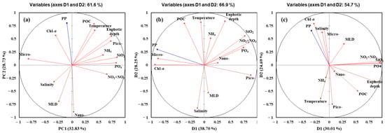
Figure 8.
Principal components analysis (PCA) ordination plots showing primary production of phytoplankton in relation to environmental and biological conditions in the YS (a), the SS (b), and the EJS (c), 2018. Micro-, nano-, and pico- represent contributions of compositions of micro-, nano-, and pico-sized phytoplankton to total chl-a; PP represents primary production.
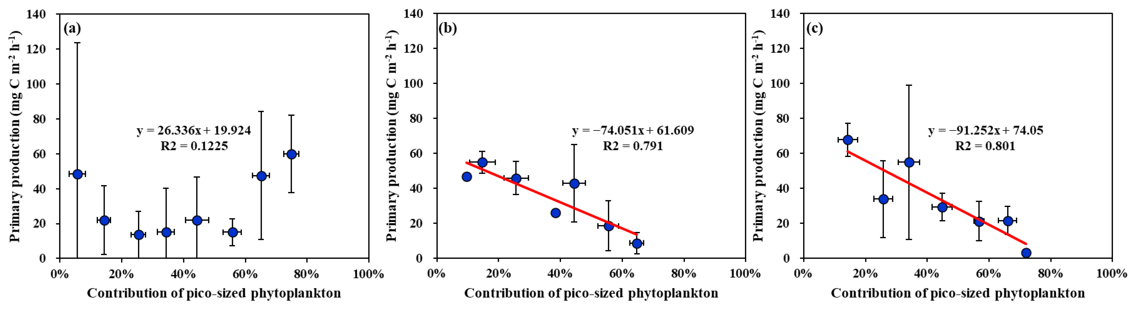
No strong correlation (R2 = 0.1225 p > 0.05) was found between the biomass contributions of pico-sized phytoplankton and the primary production of phytoplankton in the YS (Figure 9a). In contrast, significantly negative correlations between the biomass contributions of pico-sized phytoplankton and the primary production were observed in the SS (R2 = 0.791, p < 0.01) and the EJS (R2 = 0.801, p < 0.01) (Figure 9b,c).
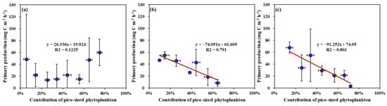
Figure 9.
Relationships between primary production and contribution of pico-sized phytoplankton (<2 μm) to total chl-a concentrations in the YS (a), the SS (b), and the EJS (c), 2018.
4. Discussion
4.1. Comparisons of Primary Production between This and Previous Studies
Based on a 10-h photoperiod and the hourly primary productions obtained in this study (Figure 6), the mean daily primary productions in the YS were 25.8 ± 11.9, 292.7 ± 393.9, 139.0 ± 66.9, and 607.5 ± 172.6 mg C m−2 d−1 during winter, spring, summer, and autumn, respectively. Our values obtained in this study were slightly lower than the ranges (56–947 mg C m−2 d−1) of the values reported previously in adjacent or nearly identical regions to our sites in the YS (Table 3). In particular, our spring (293 mg C m−2 d−1) and summer (139 mg C m−2 d−1) values in this study were significantly lower (t-test, p < 0.05) than the spring (851 ± 108 mg C m−2 d−1) and summer (555 ± 231 mg C m−2 d−1) values averaged from previous studies. These lower seasonal productions in 2018 might be explained by a recent change in the nutrient budgets in the YS. An increasing trend in dissolved inorganic nitrogen (DIN) concentration since the 1980s was reported, whereas a decreasing trend from the 1980s to 2000 followed by a slight increase in PO4 concentration was observed in the YS [16,36]. These changes in DIN and PO4 have induced a gradual increase in the N/P ratio and a shift from N-limitation to P-limitation in the YS [36]. The P-limited condition could convert dominant species of phytoplankton from diatoms to small-sized non-diatoms with higher growth rates in P-limited waters but lower photosynthetic efficiencies [18,24,37]. Lin et al. [16] reported that a dramatic decrease in primary production in the YS during all seasons between 1983–1986 and 1996–1998 periods could be one of the ecological responses caused by the increase in the N/P ratio. In this study, the N/P ratios (32 ± 14) during the spring period were significantly higher (one-sample t-test, p < 0.01) than the Redfield ratios (16) [38], which could have resulted in a limitation for diatom growth [39,40]. Indeed, the diatom compositions (approximately 50%) in the YS in spring based on the results from our parallel study (non-published data) were distinctly lower than those reported previously in 1986 (89%) and 1998 (70%) [23]. This shift in dominant species could have caused the low primary production in spring 2018. Jang et al. [24] reported that the high contribution of pico-sized (<2 μm) phytoplankton to the total primary production could induce a lower total primary production in the YS when the N/P ratio is higher than 30 during the summer period. We did not measure the production of pico-sized phytoplankton in this study, but the higher N/P ratio (54 ± 78) at upper euphotic depth (100 and 30%) accounted for about 75% of integrated primary production and could explain the lower primary production in the YS during summer 2018.
Table 3.
Comparisons of daily primary production in the YS. PP represents daily primary production.
Since the primary production measurements have rarely been conducted in the SS section belonging to the northern part of the East China Sea, we compared our results with those measured previously in the entire East China Sea (Table 4). The average daily primary productions in the SS during this observation are within the range (102–1727 mg C m−2 d−1) reported previously in the East China Sea (Table 4). However, the winter and summer values in this study were significantly lower (t-test, p < 0.05) than the mean winter (206 ± 93 mg C m−2 d−1) and summer (621 ± 179 mg C m−2 d−1) productions reported previously. In comparison, the autumn value (487 mg C m−2 d−1) in this study was consistent with the previous findings (503 ± 186 mg C m−2 d−1). For the springtime, our daily production (426 mg C m−2 d−1) was not statistically different (t-test, p > 0.05) from the mean production (350 ± 161 mg C m−2 d−1) in early spring (March), but our spring value was considerably lower than those reported previously in April (1727 mg C m−2 d−1) and May (1375 mg C m−2 d−1).
Table 4.
Comparisons of daily primary production in the East China Sea. PP represents daily primary production.
The daily primary productions measured in this study during four seasons are within the range (44–1505 mg C m−2 d−1) obtained previously from the various regions in the EJS in different seasons (Table 5). However, our value (284 mg C m−2 d−1) during the winter period was significantly higher (t-test, p < 0.05) than the winter mean value (75 ± 44 mg C m−2 d−1) reported by Nagata [51] and Yoshie et al. [52], whereas our spring (491 mg C m−2 d−1) and summer (106 mg C m−2 d−1) rates were significantly lower (t-test, p < 0.05) than the spring (858 ± 376 mg C m−2 d−1) and summer (519 ± 184 mg C m−2 d−1) values averaged from various previous studies. A plausible mechanism for the difference might be related to the development of the MLD in the EJS during the wintertime. A vigorous vertical mixing driven by the Asian winter monsoon can limit the availability of light to phytoplankton in winter [53,54] but induces an increase in the nutrient availability in the upper euphotic layer from spring to summer [55,56]. However, the MLD has been gradually decreased by an increase in water temperature and weakened wind stress in the EJS [17,57,58], which could offer better light conditions for phytoplankton growth in winter but fewer nutrients for the spring phytoplankton bloom. In this way, the difference in seasonal primary production in the EJS mentioned above could be explained by the recent change in the MLD. However, because our surveys in the EJS were restricted to only 2018, this mechanism needs to be verified by a long-term observation. Another reason for the low primary production, especially in spring 2018, could be potentially having missed the bloom timing of the phytoplankton during our observation period. In general, the spring bloom in the EJS is mainly driven by the massive growth of diatoms, which account for the majority of large-sized (> 20 μm) phytoplankton [59,60,61]. Indeed, Kwak et al. [62] observed a significantly higher contribution (approximately 60%) of diatoms during the spring bloom period than in other seasons. In this study, the contribution of the large-sized phytoplankton was rather lower during the spring (Figure 5c). However, much lower diatom contributions were detected based on our parallel stud, showing that diatoms accounted for only 23.1% (± 9.9%) of total phytoplankton communities in the EJS in spring (non-published data). The other reason might be conspicuously low phytoplankton biomass in the EJS in April 2018. Based on MODIS (Moderate Resolution Imaging Spectrometer)-Aqua monthly level-3 datasets regarding chl-a (https://oceandata.sci.gsfc.nasa.gov/MODIS-Aqua/, accessed on 3 August 2021), the surface chl-a showed strong negative anomalies in the southwestern part of the EJS during April between 2003–2015 and 2018 (data not shown). As the chl-a concentrations in the EJS were one of the major factors controlling the primary production (Figure 8c), a noticeable low chl-a concentration could cause lower primary production in the EJS during the springtime in 2018. At the current stage, it is difficult to find out a solid reason for the low chl-a concentration in the EJS during April 2018, which should be further resolved for a better understanding of the EJS ecosystem.
Table 5.
Comparisons of daily primary production in the EJS. PP represents daily primary production.
4.2. Main Factors Affecting the Primary Production in the YS, SS, and EJS in 2018
Based on the PCA results (Figure 8), the major factors controlling the phytoplankton productions were different among the three seas. Total chl-a concentrations (positively; +), temperature (+), MLD (negatively; −), and nano-sized phytoplankton contribution (−) are found to be major controlling factors in the YS. In comparison, total chl-a concentrations (+), pico- (−) and micro-sized (+) phytoplankton contributions, and nutrients (−) except for NH4 can greatlyaffect the primary production in the SS. For the EJS, the primary production of phytoplankton can greatly vary due to total chl-a concentrations (+), micro-sized phytoplankton contribution (+), salinity (+), pico-sized phytoplankton (−), and water temperature (−). The effects of physical (temperature, salinity, and MLD) and chemical (nutrients) factors are different in the YS, the SS, and the EJS. Given the positive relationships between the primary productions and the total chl-a concentrations in this study, biomass-driven primary productions are characteristics in the YS, the SS, and the EJS ecosystems, at least in 2018. However, the effects of the three size groups of phytoplankton can be different among the three seas. The contribution of nano-sized phytoplankton in the YS and the contributions of pico-sized phytoplankton in the SS and the EJS are negatively correlated with the primary productions in this study. Choi et al. [42] reported nano-phytoplankton contributed greatly to the primary production in the YS, based on the large biomass contribution of nano-phytoplankton (approximately 60%). In this study, the negative relationship between the nano-sized phytoplankton contribution and the primary production indicates that increasing contributions of the nano-sized phytoplankton could decrease the primary production in the YS. In the EJS, several previous studies reported higher contributions of pico-sized phytoplankton could cause a decrease in the primary production [12,22,69]. Indeed, marked decreasing trends in the primary productions with increasing pico-sized phytoplankton biomass were observed in the SS and EJS during our observation period in 2018 (Figure 9b.c). This could be caused by the different primary productivities between pico- and large-sized (>2 μm) phytoplankton [22]. Generally, pico-sized phytoplankton have a lower primary productivity than large phytoplankton [14,22,70]. Therefore, the total primary production can be decreased by increasing contribution of pico-sized phytoplankton, with their lower productivity traits. Under ongoing warming ocean conditions, pico-sized phytoplankton are expected to be predominant in phytoplankton communities [71,72,73,74]. In this pico-sized-phytoplankton-dominated ecosystem, a lower total primary production could be expected in the SS and the EJS based on the negative relationships between the primary production and pico-sized phytoplankton observed in this study. The ecological roles of pico-sized phytoplankton in regional marine ecosystems should be further investigated in the YS, the SS, and the EJS with current environmental changes.
Author Contributions
Conceptualization, H.-K.J. and S.-H.L.; methodology, H.-K.J.; validation, H.-K.J. and S.-H.L.; formal analysis, H.-K.J.; investigation, H.-K.J., Y.K., H.J., J.-J.K., D.L., N.J., K.K., M.-J.K. and S.K.; data curation, H.-K.J.; writing—original draft preparation, H.-K.J.; writing—review and editing, S.-H.L.; visualization, H.-K.J.; supervision, S.-H.L.; project administration, S.-H.Y. and S.-H.L.; funding acquisition, S.-H.Y. and S.-H.L. All authors have read and agreed to the published version of the manuscript.
Funding
This research was fundedby the National Institute of Fisheries Science (‘Development of marine ecological forecasting system for Korean waters’; R2021068).
Institutional Review Board Statement
Not applicable.
Informed Consent Statement
Not applicable.
Data Availability Statement
Not applicable.
Acknowledgments
We appreciate the captains and crew of R/V Tamgu 3 and 8 for their assistance in collecting our samples. We would also like to thank the researchers in the NIFS for their assistance with sample analysis. This work was supported by the National Institute of Fisheries Science (NIFS) grant (‘Development of marine ecological forecasting system for Korean waters’; R2021068) funded by the Ministry of Oceans and Fisheries, Republic of Korea.
Conflicts of Interest
The authors declare no conflict of interest.
References
- Falkowski, P.G.; Barber, R.T.; Smetacek, V. Biogeochemical controls and feedbacks on ocean primary production. Science 1998, 281, 200–206. [Google Scholar] [CrossRef] [Green Version]
- Behrenfeld, M.J.; Randerson, J.T.; McClain, C.R.; Feldman, G.C.; Los, S.O.; Tucker, C.J.; Falkowski, P.G.; Field, C.B.; Frouin, R.; Esaias, W.E.; et al. Biospheric primary production during an ENSO transition. Science 2001, 291, 2594–2597. [Google Scholar] [CrossRef] [PubMed] [Green Version]
- Nixon, S.; Thomas, A. On the size of the Peru upwelling ecosystem. Deep. Res. Part I Oceanogr. Res. Pap. 2001, 48, 2521–2528. [Google Scholar] [CrossRef]
- Gong, G.C.; Wen, Y.H.; Wang, B.W.; Liu, G.J. Seasonal variation of chlorophyll a concentration, primary production and environmental conditions in the subtropical East China Sea. Deep. Res. Part II Top. Stud. Oceanogr. 2003, 50, 1219–1236. [Google Scholar] [CrossRef]
- Tremblay, J.É.; Robert, D.; Varela, D.E.; Lovejoy, C.; Darnis, G.; Nelson, R.J.; Sastri, A.R. Current state and trends in Canadian Arctic marine ecosystems: I. Primary production. Clim. Chang. 2012, 115, 161–178. [Google Scholar] [CrossRef] [Green Version]
- Kleppel, G.S.; Burkart, C.A. Egg production and the nutritional environment of Acartia tonsa: The role of food quality in copepod nutrition. ICES J. Mar. Sci. 1995, 52, 297–304. [Google Scholar] [CrossRef]
- Kang, J.J.; Joo, H.T.; Lee, J.H.; Lee, J.H.; Lee, H.W.; Lee, D.; Kang, C.K.; Yun, M.S.; Lee, S.H. Comparison of biochemical compositions of phytoplankton during spring and fall seasons in the northern East/Japan Sea. Deep. Res. Part II Top. Stud. Oceanogr. 2017, 143, 73–81. [Google Scholar] [CrossRef]
- Lee, D.; Son, S.H.; Kim, W.; Park, J.M.; Joo, H.; Lee, S.H. Spatio-temporal variability of the habitat suitability index for chub mackerel (Scomber Japonicus) in the East/Japan Sea and the South Sea of South Korea. Remote Sens. 2018, 10, 938. [Google Scholar] [CrossRef] [Green Version]
- Lee, D.; Son, S.H.; Lee, C., Il; Kang, C.K.; Lee, S.H. Spatio-temporal variability of the habitat suitability index for the Todarodes pacificus (Japanese Common Squid) around South Korea. Remote Sens. 2019, 11, 2720. [Google Scholar] [CrossRef] [Green Version]
- Lee, S.H.; Yun, M.S.; Kim, B.K.; Saitoh, S.I.; Kang, C.K.; Kang, S.H.; Whitledge, T. Latitudinal carbon productivity in the Bering and Chukchi Seas during the summer in 2007. Cont. Shelf Res. 2013, 59, 28–36. [Google Scholar] [CrossRef]
- Kim, B.K.; Joo, H.T.; Song, H.J.; Yang, E.J.; Lee, S.H.; Hahm, D.; Rhee, T.S.; Lee, S.H. Large seasonal variation in phytoplankton production in the Amundsen Sea. Polar Biol. 2015, 38, 319–331. [Google Scholar] [CrossRef]
- Kang, J.J.; Jang, H.K.; Lim, J.H.; Lee, D.; Lee, J.H.; Bae, H.; Lee, C.H.; Kang, C.K.; Lee, S.H. Characteristics of Different Size Phytoplankton for Primary Production and Biochemical Compositions in the Western East/Japan Sea. Front. Microbiol. 2020, 11, 1–16. [Google Scholar] [CrossRef]
- Taniguchi, A. Geographical variation of primary production in the Western Pacific Ocean and adjacent seas with reference to the inter-relations between various parameters of primary production. Mem. Fac. Fish. Hokkaido Univ. 1972, 19, 1–33. [Google Scholar]
- Lee, S.H.; Sun Yun, M.; Kyung Kim, B.; Joo, H.T.; Kang, S.H.; Keun Kang, C.; Whitledge, T.E. Contribution of small phytoplankton to total primary production in the Chukchi Sea. Cont. Shelf Res. 2013, 68, 43–50. [Google Scholar] [CrossRef]
- Belkin, I.M. Rapid warming of Large Marine Ecosystems. Prog. Oceanogr. 2009, 81, 207–213. [Google Scholar] [CrossRef]
- Lin, C.; Ning, X.; Su, J.; Lin, Y.; Xu, B. Environmental changes and the responses of the ecosystems of the Yellow Sea during 1976–2000. J. Mar. Syst. 2005, 55, 223–234. [Google Scholar] [CrossRef]
- Chang, P.H.; Cho, C.H.; Ryoo, S.B. Recent changes of mixed layer depth in the East/Japan Sea: 1994-2007. Asia-Pac. J. Atmos. Sci. 2011, 47, 497–501. [Google Scholar] [CrossRef]
- Jin, J.; Liu, S.M.; Ren, J.L.; Liu, C.G.; Zhang, J.; Zhang, G.L.; Huang, D.J. Nutrient dynamics and coupling with phytoplankton species composition during the spring blooms in the Yellow Sea. Deep. Res. Part II Top. Stud. Oceanogr. 2013, 97, 16–32. [Google Scholar] [CrossRef]
- Kim, J.Y.; Kang, D.J.; Lee, T.; Kim, K.R. Long-term trend of CO2 and ocean acidification in the surface water of the Ulleung Basin, the East/Japan Sea inferred from the underway observational data. Biogeosciences 2014, 11, 2443–2454. [Google Scholar] [CrossRef] [Green Version]
- Chiba, S.; Batten, S.; Sasaoka, K.; Sasai, Y.; Sugisaki, H. Influence of the Pacific Decadal Oscillation on phytoplankton phenology and community structure in the western North Pacific. Geophys. Res. Lett. 2012, 39, 2–7. [Google Scholar] [CrossRef]
- Doney, S.C.; Ruckelshaus, M.; Emmett Duffy, J.; Barry, J.P.; Chan, F.; English, C.A.; Galindo, H.M.; Grebmeier, J.M.; Hollowed, A.B.; Knowlton, N.; et al. Climate change impacts on marine ecosystems. Ann. Rev. Mar. Sci. 2012, 4, 11–37. [Google Scholar] [CrossRef] [Green Version]
- Lee, S.H.; Joo, H.T.; Lee, J.H.; Lee, J.H.; Kang, J.J.; Lee, H.W.; Lee, D.; Kang, C.K. Seasonal carbon uptake rates of phytoplankton in the northern East/Japan Sea. Deep. Res. Part II Top. Stud. Oceanogr. 2017, 143, 45–53. [Google Scholar] [CrossRef]
- Wang, J. Study on phytoplankton in the Yellow Sea in spring. Mar. Fisher. Res. 2001, 22, 56–61. [Google Scholar]
- Jang, H.K.; Kang, J.J.; Lee, J.H.; Kim, M.; Ahn, S.H.; Jeong, J.Y.; Yun, M.S.; Han, I.S.; Lee, S.H. Recent Primary Production and Small Phytoplankton Contribution in the Yellow Sea during the Summer in 2016. Ocean Sci. J. 2018, 53, 509–519. [Google Scholar] [CrossRef]
- Lee, S.H.; Son, S.; Dahms, H.U.; Park, J.W.; Lim, J.H.; Noh, J.H.; Kwon, J.I.; Joo, H.T.; Jeong, J.Y.; Kang, C.K. Decadal changes of phytoplankton chlorophyll-a in the East Sea/Sea of Japan. Oceanology 2014, 54, 771–779. [Google Scholar] [CrossRef]
- Joo, H.T.; Son, S.H.; Park, J.W.; Kang, J.J.; Jeong, J.Y.; Lee, C., Il; Kang, C.K.; Lee, S.H. Long-term pattern of primary productivity in the East/Japan sea based on ocean color data derived from MODIS-Aqua. Remote Sens. 2016, 8, 25. [Google Scholar] [CrossRef] [Green Version]
- Levitus, S. Climatological Atlas of the World Ocean; NOAA Prof. Paper 13; U.S. Government Printing Office: Washington, DC, USA, 1982; 173p.
- Gardner, W.D.; Chung, S.P.; Richardson, M.J.; Walsh, I.D. The oceanic mixed-layer pump. Deep. Res. Part II 1995, 42, 757–775. [Google Scholar] [CrossRef]
- Parsons, T.R.; Maita, Y.; Lalli, C.M. A Manual of Biological and Chemical Methods for Seawater Analysis; Pergamon Press: Oxford, UK, 1984. [Google Scholar]
- Dugdale, R.C.; Goering, J.J. Uptake of New and Regenerated Forms of Nitrogen in Primary Productivity. Limnol. Oceanogr. 1967, 12, 196–206. [Google Scholar] [CrossRef] [Green Version]
- Hama, T.; Miyazaki, T.; Ogawa, Y.; Iwakuma, T.; Takahashi, M.; Otsuki, A.; Ichimura, S. Measurement of photosynthetic production of a marine phytoplankton population using as Table 13C isotope. Mar. Biol. 1983, 73, 31–36. [Google Scholar] [CrossRef]
- Garneau, M.È.; Gosselin, M.; Klein, B.; Tremblay, J.É.; Fouilland, E. New and regenerated production during a late summer bloom in an Arctic polynya. Mar. Ecol. Prog. Ser. 2007, 345, 13–26. [Google Scholar] [CrossRef]
- Li, W.K.W.; Irwin, B.D.; Dickie, P.M. Dark fixation of 14C: Variations related to biomass and productivity of phytoplankton and bacteria. Limnol. Oceanogr. 1993, 38, 483–494. [Google Scholar] [CrossRef] [Green Version]
- Gosselin, M.; Levasseur, M.; Wheeler, P.A. Deep Sea Research Part II: Topical Studies in Oceanography—New measurements of phytoplankton and ice algal production in the Arctic Ocean. Deep Sea Res. Part II Top. Stud. Oceanogr. 1997, 44, 1623–1644. [Google Scholar] [CrossRef]
- Lee, H.W.; Noh, J.H.; Choi, D.H.; Yun, M.; Bhavya, P.S.; Kang, J.J.; Lee, J.H.; Kim, K.W.; Jang, H.K.; Lee, S.H. Picocyanobacterial contribution to the total primary production in the northwestern pacific ocean. Water 2021, 13, 1610. [Google Scholar] [CrossRef]
- Wei, Q.; Yao, Q.; Wang, B.; Wang, H.; Yu, Z. Long-term variation of nutrients in the southern Yellow Sea. Cont. Shelf Res. 2015, 111, 184–196. [Google Scholar] [CrossRef]
- Tao, F.; Daoji, L.; Lihua, Y.; Lei, G.; Lihua, Z. Effects of irradiance and phosphate on growth of nanophytoplankton and picophytoplankton. Acta Ecol. Sin. 2006, 26, 2783–2789. [Google Scholar] [CrossRef]
- Redfeild, A. The influence of organisms on the composition of sea water. Sea 1963, 2, 26–77. [Google Scholar]
- Egge, J.K. Are diatoms poor competitors at low phosphate concentrations? J. Mar. Syst. 1998, 16, 191–198. [Google Scholar] [CrossRef]
- Zhou, M.-j.; Shen, Z.-l.; Yu, R.-c. Responses of a coastal phytoplankton community to increased nutrient input from the Changjiang (Yangtze) River. Cont. Shelf Res. 2008, 28, 1483–1489. [Google Scholar] [CrossRef]
- Kang, Y.S.; Choi, J.K.; Chung, K.H.; Park, Y.C. Primary productivity and assimilation umber in the Kyonggi bay and the mid-eastern coast of Yellow Sea. J. Oceanogr. Soc. Korea 1992, 27, 237–246. [Google Scholar]
- Choi, J.K.; Noh, J.H.; Shin, K.S.; Hong, K.H. The early autumn distribution of chlorophyll-a and primary productivity in the Yellow Sea, 1992. The Yellow Sea 1995, 1, 68–80. [Google Scholar]
- Choi, J.K.; Noh, J.H.; Cho, S.H. Temporal and spatial variation of primary production in the Yellow Sea. The present and the future of yellow sea environments. In Proceedings of the Yellow Sea International Symposium, Ansan, Korea, 6–7 November 2003; Korea Ocean R&D Institute: Seoul, Korea, 2003; pp. 103–115. [Google Scholar]
- Son, S.H.; Campbell, J.; Dowell, M.; Yoo, S.; Noh, J. Primary production in the Yellow Sea determined by ocean color remote sensing. Mar. Ecol. Prog. Ser. 2005, 303, 91–103. [Google Scholar] [CrossRef]
- Lee, Y. Phytoplankton Dynamics and Primary Production in the Yellow Sea during Winter and Summer. Unpublished Ph.D. Thsesis, Inha University, Incheon, Korea, August 2012. [Google Scholar]
- Chung, C.S.; Yang, D.B. On the primary productivity in the southern sea of Korea. J. Oceanogr. Soc. Korea 1991, 26, 242–254. [Google Scholar]
- Hama, T.; Shin, K.H.; Handa, N. Spatial variability in the primary productivity in the East China Sea and its adjacent waters. J. Oceanogr. 1997, 53, 41–51. [Google Scholar] [CrossRef]
- Lee Chen, Y.L.; Chen, H.Y. Nitrate-based new production and its relationship to primary production and chemical hydrography in spring and fall in the East China Sea. Deep. Res. Part II Top. Stud. Oceanogr. 2003, 50, 1249–1264. [Google Scholar] [CrossRef]
- Siswanto, E.; Ishizaka, J.; Yokouchi, K. Estimating chlorophyll-a vertical profiles from satellite data and the implication for primary production in the Kuroshio front of the East China Sea. J. Oceanogr. 2005, 61, 575–589. [Google Scholar] [CrossRef]
- Zhang, Y.R.; Ding, Y.P.; Li, T.J.; Xue, B.; Euo, Y.M. Annual variations of chlorophyll a and primary productivity in the East China Sea. Oceanol. Limno. Sin. 2016, 47, 261–268. [Google Scholar] [CrossRef]
- Nagata, H. the Yamato Rise, central Japan Sea. Plankton Bio. Ecol. 1998, 45, 159–170. [Google Scholar]
- Yoshie, N.; Shin, K.H.; Noriki, S. Seasonal variations of primary productivity and assimilation numbers in the western North Pacific. Spec. Rep. Reg. Stud. North-East Eurasia North Pac. Hokkaido Univ. 1999, 1, 49–62. [Google Scholar]
- Sverdrup, H.U. On conditions for the vernal blooming of phytoplankton. ICES J. Mar. Sci. 1953, 18, 287–295. [Google Scholar] [CrossRef]
- Yentsch, C.S. Estimates of “new production” in the mid-North Atlantic. J. Plankton Res. 1990, 12, 717–734. [Google Scholar] [CrossRef]
- Nishikawa, H.; Yasuda, I.; Komatsu, K.; Sasaki, H.; Sasai, Y.; Setou, T.; Shimizu, M. Winter mixed layer depth and spring bloom along the Kuroshio front: Implications for the Japanese sardine stock. Mar. Ecol. Prog. Ser. 2013, 487, 217–229. [Google Scholar] [CrossRef] [Green Version]
- Mayot, N.; D’Ortenzio, F.; Uitz, J.; Gentili, B.; Ras, J.; Vellucci, V.; Golbol, M.; Antoine, D.; Claustre, H. Influence of the Phytoplankton Community Structure on the Spring and Annual Primary Production in the Northwestern Mediterranean Sea. J. Geophys. Res. Ocean. 2017, 122, 9918–9936. [Google Scholar] [CrossRef] [Green Version]
- Lim, S.H.; Jang, C.J.; Oh, I.S.; Park, J.J. Climatology of the mixed layer depth in the East/Japan Sea. J. Mar. Syst. 2012, 96–97, 1–14. [Google Scholar] [CrossRef]
- Bae, H.; Lee, D.; Kang, J.J.; Lee, J.H.; Jo, N.; Kim, K.; Jang, H.K.; Kim, M.J.; Kim, Y.; Kwon, J., Il; et al. Satellite-derived protein concentration of phytoplankton in the Southwestern East/Japan Sea. J. Mar. Sci. Eng. 2021, 9, 189. [Google Scholar] [CrossRef]
- Kang, Y.-S.; Choi, H.-C.; Lim, J.-H.; Jeon, I.-S.; Seo, J.-H. Dynamics of the Phytoplankton Community in the Coastal Waters of Chuksan Harbor, East Sea. Algae 2005, 20, 345–352. [Google Scholar] [CrossRef]
- Zuenko, Y.; Selina, M.; Stonik, I. On conditions of phytoplankton blooms in the coastal waters of the north-western East/Japan Sea. Ocean Sci. J. 2006, 41, 31–41. [Google Scholar] [CrossRef]
- Chang, K.-I.; Zhang, C.-I.; Park, C.; Kang, D.-J.; Ju, S.-J.; Lee, S.-H.; Wimbush, M. (Eds.) Oceanography of the East Sea (Japan Sea), 1st ed.; Springer International Publishing: Cham, Switzerland, 2016. [Google Scholar]
- Kwak, J.H.; Han, E.; Lee, S.H.; Park, H.J.; Kim, K.R.; Kang, C.K. A consistent structure of phytoplankton communities across the warm–cold regions of the water mass on a meridional transect in the East/Japan Sea. Deep. Res. Part II Top. Stud. Oceanogr. 2017, 143, 36–44. [Google Scholar] [CrossRef]
- Chung, C.S.; Shim, J.H.; Park, Y.H.; Park, S.G. Primary productivity and nitrogenous nutrient dynamics in the East Sea of Korea. J. Oceanogr Soc. Korea 1989, 24, 52–61. [Google Scholar]
- Park, J.S.; Kang, C.K.; An, K.H. Community structure and spatial distribution of phytoplankton in the polar front region off the east coast of Korea in summer. Bull. Korean Fish. Soc. 1991, 24, 237–247. [Google Scholar]
- Yamada, K.; Ishizaka, J.; Nagata, H. Spatial and temporal variability of satellite primary production in the Japan Sea from 1998 to 2002. J. Oceanogr. 2005, 61, 857–869. [Google Scholar] [CrossRef]
- Hyun, J.H.; Kim, D.; Shin, C.W.; Noh, J.H.; Yang, E.J.; Mok, J.S.; Kim, S.H.; Kim, H.C.; Yoo, S. Enhanced phytoplankton and bacterioplankton production coupled to coastal upwelling and an anticyclonic eddy in the Ulleung basin. East Sea Aquat. Microb. Ecol. 2009, 54, 45–54. [Google Scholar] [CrossRef]
- Kwak, J.H.; Lee, S.H.; Park, H.J.; Choy, E.J.; Jeong, H.D.; Kim, K.R.; Kang, C.K. Monthly measured primary and new productivities in the Ulleung Basin as a biological “hot spot” in the East/Japan Sea. Biogeosciences 2013, 10, 4405–4417. [Google Scholar] [CrossRef] [Green Version]
- Kwak, J.H.; Hwang, J.; Choy, E.J.; Park, H.J.; Kang, D.J.; Lee, T.; Chang, K., Il; Kim, K.R.; Kang, C.K. High primary productivity and f-ratio in summer in the Ulleung basin of the East/Japan Sea. Deep. Res. Part I Oceanogr. Res. Pap. 2013, 79, 74–785. [Google Scholar] [CrossRef]
- Joo, H.T.; Son, S.H.; Park, J.W.; Kang, J.J.; Jeong, J.Y.; Kwon, J., Il; Kang, C.K.; Lee, S.H. Small phytoplankton contribution to the total primary production in the highly productive Ulleung Basin in the East/Japan Sea. Deep. Res. Part. II Top. Stud. Oceanogr. 2017, 143, 54–61. [Google Scholar] [CrossRef]
- Lim, Y.J.; Kim, T.W.; Lee, S.H.; Lee, D.; Park, J.; Kim, B.K.; Kim, K.; Jang, H.K.; Bhavya, P.S.; Lee, S.H. Seasonal Variations in the Small Phytoplankton Contribution to the Total Primary Production in the Amundsen Sea, Antarctica. J. Geophys. Res. Ocean. 2019, 124, 8324–8341. [Google Scholar] [CrossRef]
- Agawin, N.S.R.; Duarte, C.M.; Agusti, S. Nutrient and temperature control of the contribution of picoplankton to phytoplankton biomass and production. Limnol. Oceanogr. 2000, 45, 591–600. [Google Scholar] [CrossRef]
- Hilligsøe, K.M.; Richardson, K.; Bendtsen, J.; Sørensen, L.L.; Nielsen, T.G.; Lyngsgaard, M.M. Linking phytoplankton community size composition with temperature, plankton food web structure and sea-air CO2 flux. Deep. Res. Part I Oceanogr. Res. Pap. 2011, 58, 826–838. [Google Scholar] [CrossRef]
- Morán, X.A.G.; López-Urrutia, Á.; Calvo-Díaz, A.; LI, W.K.W. Increasing importance of small phytoplankton in a warmer ocean. Glob. Chang. Biol. 2010, 16, 1137–1144. [Google Scholar] [CrossRef]
- Mousing, E.A.; Ellegaard, M.; Richardson, K. Global patterns in phytoplankton community size Structure-evidence for a direct temperature effect. Mar. Ecol. Prog. Ser. 2014, 497, 25–38. [Google Scholar] [CrossRef] [Green Version]


Publisher’s Note: MDPI stays neutral with regard to jurisdictional claims in published maps and institutional affiliations. |
© 2021 by the authors. Licensee MDPI, Basel, Switzerland. This article is an open access article distributed under the terms and conditions of the Creative Commons Attribution (CC BY) license (https://creativecommons.org/licenses/by/4.0/).